


1. Introduction
1.1 Background and overview
Fireball camera networks consist of a widely spaced array of all-sky astronomical optical instruments designed to observe incoming meteors leading to the recovery of fresh meteorite falls, with associated orbits. A fresh, uncontaminated meteorite associated with a known orbit provides valuable information about the composition and formation of the Solar System.
Several major fireball networks have been in operation throughout recent history, and today many regional networks exist utilising still and video technology, including the Desert Fireball Network (DFN) in the Australian outback (Oberst et al. Reference Oberst1998; Trigo-Rodríguez et al. Reference Trigo-Rodriguez, Llorca, Castro-Tirado, Ortiz, Docobo and Fabregat2006; Weryk et al. Reference Weryk, Brown, Domokos, Edwards, Krzeminski, Nudds and Welch2007; Cooke & Moser Reference Cooke and Moser2011; Jenniskens et al. Reference Jenniskens, Gural, Dynneson, Grigsby, Newman, Borden, Koop and Holman2011; Bland et al. Reference Bland2012; Colas et al. Reference Colas2014). The DFN has unique constraints and advantages over other networks; the Australian continent is ideally suited to meteorite recovery, due to large areas of low vegetation with pale colour rocks, making meteorite detection easier, and good weather, giving both a greater percentage of clear nights for observations, and also lower chance of meteorite contamination due to precipitation. Conversely, the large distances and remote nature of the Australian outback pose logistical and communication challenges.
Considering data analysis, early fireball networks (the earliest of which began in the 1960s) were film-based, using long exposures, typically all night. Images were inspected manually, and negatives with fireballs were then scanned and processed by hand (Spurný, Borovička, & Shrbený Reference Spurný, Borovička and Shrbený2007). For film systems, a supplementary brightness sensor, such as a photomultiplier tube, is used to detect events and provide time brackets for an operator to review the films. Images were then calibrated by comparison of the streaks left by long exposure stars with the known star positions and exposure start/end times. Data reduction and fireball detection involved considerable manual activity for each fireball. More recently in the digital age, video systems are prevalent, and there are several extant software tools specifically for fireball detection, such as METREC (Molau Reference Molau1998) or more recently UFOCapture (SonotaCo, Japan) or ASGARD (Brown et al. Reference Brown, Weryk, Kohut, Edwards and Krzeminski2010). One can also use generic motion detection software, as used on many security camera systems. Video systems have sufficient resolution to usefully calculate fireball orbits, but generally lack the resolution to capture fully the final stages of ablation. This precision is needed for meteorite recovery, unless the cameras are placed relatively closely together (typically less than 50 km), or the fireball is particularly big, to ensure proximity in the final stages of meteoroid ablation. This is impractical for the DFN, which covers large areas of the sparsely populated Australian outback. Instead of video, the DFN instead uses high-resolution still images, from a commercial DSLR system (currently Nikon D810 taking 25 s exposures every 30 s), and uses an innovative technique using a liquid crystal shutter to embed absolute timing information of the fireball within the exposure (Howie et al. Reference Howie, Paxman, Bland, Towner, Cupak, Sansom and Devillepoix2017a). The higher resolution of the DSLR compared to video allows a larger camera spacing of about 100–150 km, while still observing fireballs with enough precision to give a reasonable chance of meteorite recovery. The use of the liquid crystal shutter to give precise timing also enables corroboration of events using video cameras as well, allowing a mix of systems to be deployed.
Such a system still requires software to detect fireball events automatically, unless one is manually surveying many thousands of images. The core of event detection for video systems is around changing pixels and motion detection. This can be coupled with real-time smoothing/noise removal, and tracking of motion over multiple frames, to remove short-lived false positives. Real-time processing of video systems requires significant processing and storage capability, for example, recommended systems requirements for UFOCapture are 2.4 GHz Pentium 4 for a 640 × 480 resolution video system. In the case of long exposure still images, the ‘number of frames’ is significantly fewer, so more time can be devoted to analysing each image, but the basic approach used is similar: one searches for changes between frames, and localises and categorises them.
Machine learning was defined by Arthur Samuel in 1959 as a ‘field of study that gives computers the ability to learn without being explicitly programmed’ (Samuel Reference Samuel1959). It has been implemented in a wide variety of application areas, from medicine to pedestrian detection in advertising (Perlich et al. Reference Perlich, Dalessandro, Raeder, Stitelman and Provost2014), finance (Clémençon Reference Cl’emençon2015), military (DesJardins Reference DesJardins1997), and astronomy (Ball & Brunner Reference Ball and Brunner2010). The potential of machine learning is being developed at every level within the era of big data management. Machine learning algorithms are categorised in three main classes: supervised learning, unsupervised learning, and reinforcement learning algorithms. For fireball detection, a supervised learning approach appears best suited, as the algorithm can be presented with training data that have been categorised by a human. Additionally, it is also one of the least computationally expensive approaches which matches well with the hardware requirements of solar-powered remote camera systems that make up the majority of the DFN observatories. In supervised learning, the computer is presented with a set of sample data and its corresponding output, forming a training set. The computer will then improve its prediction accuracy by reducing the error between the predicted value and the correctly labelled value, to reach a general model that best maps inputs to outputs (Bishop Reference Bishop2006). For the DFN pipeline, a binary classifier is appropriate: to indicate fireball or non-fireball when presented with an image.
There appears to be little previous application to fireball image detection to date. The only publication the authors are aware of is Zhao (Reference Zhao2010), who applied support vector machine classification algorithms to give the computer the ability to learn how to cluster fireball event data obtained from RADAR observations. This work appears to have been successful in the identification of meteors with a trajectory perpendicular to the RADAR beam but had difficulties in the detection of other meteor trails due to the poor quality of the source data.
Machine learning has potential to improve data throughput and better handle ‘strange looking fireballs’, where the possible variety of shapes, colours, and textures of fireballs can cause difficulties for traditional processing methods that expect a simple straight-line, non-fragmenting fireball. However, when considering the trade-off between traditional approaches and machine learning, one must be cognisant that machine learning can be hardware-intensive, which can be an issue for remote camera systems such as the DFN which rely on solar panels and batteries. Here, we implement both a traditional image processing approach and a simple neural network algorithm and compare the relative detection efficiencies on real data from the DFN.
1.2 Hardware constraints on a remote camera system
For the DFN systems, the cameras are located at remote sites across the Australian outback, with limited power and communication. The camera systems are typically powered by solar panels and batteries, and communications are via mobile data service, which is of somewhat erratic performance in central Australia. Hence, the deployed systems must be highly autonomous and robust, and operate with a low bandwidth while still providing timely information concerning any possible fireballs. The success of the project depends on coverage of a large area at optimal cost, which requires limited team members and many cameras, leading to the driving requirement of a highly automated, low-cost camera network. Details of the hardware are described in Howie et al. (Reference Howie, Paxman, Bland, Towner, Cupak, Sansom and Devillepoix2017b).
Due to bandwidth constraints, the full-resolution images cannot be transferred and processed centrally. This leads to the requirement of being able to carry out on-board processing of a full night s worth of images every 24 h, to keep up with data collection. Instead, only low volume event data such as lists of times and coordinates can be transferred. In opposition to this requirement for processing high volumes of data, the remote deployment requires that the system is relatively low power, to reduce unit cost of ancillary power systems. This leads to use of a low-power, low-cost, single-board computer. Currently, the DFN uses a Commell LE-37D board with a Atom N2930 1.83 GHz processor using 15 W in total. In turn, this low processing capability and time constraints lead to the development of energy-efficient techniques of fireball detection. But note that event detection is not the only task for the computer; in particular, data must be transferred from the DSLR camera to the local drive in a timely manner, to keep up with daily operations. Additionally, processed images must be moved on a daily schedule onto an external drive for long-term storage. Howie et al. (Reference Howie, Paxman, Bland, Towner, Cupak, Sansom and Devillepoix2017b) discussed the hardware design requirements in more detail.
Practical project and cost constraints on the network architecture are also a factor: if the unit cost of an observing system is too high, not enough units can be deployed to cover a large observing area, and not enough meteorite falls will be observed within the timescale of the project. Conversely, an extremely small, cheap unit would permit many systems to be deployed, but will probably have a lower performance, meaning that sites will have to be closer together to ensure sufficient accuracy of observations for meteorite recovery. This will also have a logistical (and hence cost) impact for operations and servicing in the Australian outback, as many more sites will need to be visited routinely. Furthermore at a practical project timescale level, extended development time of a prototype system represents a lost opportunity cost of not deploying a system earlier and observing a rare fireball that would otherwise be missed. With this in mind, it was decided to develop systems rapidly with tools in a relatively high-level language, even at the cost of a slightly more expensive resource hungry processor.
1.3 Human resource constraints on a data pipeline
Compared to a film-based network, a digital camera network will produce many more images, of order 1 000 per camera per night compared to 1 image per camera per night. With automated event detection, any manual steps in the rest of data processing pipeline such as event correlation and analysis become a constraint, incompatible with a large network operated by a small team. Staff are expensive, compared to computation, so fuller automation can decouple the number of cameras from number of staff needed, allowing a larger and more cost-effective network. Hence, as much of the data pipeline as is feasible should be automated, even if initial set-up costs are higher. This also has implications for network topography in terms of connectivity and the capabilities of any centralised server, which must be capable of handling data flows in a timely manner and keeping track of incomplete tasks in an environment where camera–server communications may be unreliable.
1.4 Metrics of success as applied to the DFN
The overarching goal of the event detection schema is to highlight fireballs—in the case of the DFN, the project’s primary goal is meteorite recovery, which effectively means large fireballs are the highest priority (small fireballs will not drop a meteorite). Larger fireballs are relatively rare events, so it is critical not to miss them, even at the expense of multiple false alarms. Hence, the goal of the DFN processing pipeline is to minimise the false negatives, missing a genuine rare significant fireball is a major failure, while erroneously generating false positives is undesirable, but not catastrophic. However, one must also constrain the false positives in some manner, otherwise the system will be overloaded with false positives, and the genuine fireballs will be lost in the noise, and the bandwidth resource requirements will also be onerous. In Section 4, we discuss in detail the utility of combining multiple camera event detections, to help overcome the finite chances of a single camera missing a fireball: multiple cameras can greatly improve the chances of recovering a large fireball, as only one camera of multiple possible observers needs to detect an event. This provides some constraint on acceptable values for false negatives and false positives. Additional constraints come from the likely number of meteorite falls, given the network detecting area and number of cameras. For a roughly 50 camera network like the DFN, over an area of Australia of approximately 2.5 million square km, we would expect roughly one meteorite-dropping fireball per month (Halliday, Blackwell, & Griffin Reference Halliday, Blackwell and Griffin1989) (although this would include meteorites that are too small for a practicable ground search). Acceptable false positives numbers can be quite high, as data volumes for a processed fireball are small, essentially just lists of coordinates.
2. Event detection methods
2.1 Traditional computation
Here we describe an event detection method based on a chain of image processing operations. The philosophy that has evolved is to process each still image using a chain of increasingly computationally expensive operations on fewer and fewer pixels, such that simple initial tests are used to exclude as much of the image as possible early in processing. The software is implemented in Python, using OpenCV, SciPy/NumPy, and the scikit-image libraries (Virtanen et al. Reference Virtanen2019; Oliphant Reference Oliphant2007; van der Walt et al. Reference van der Walt2014). The use of Python with NumPy allows C comparable performance but reduced development time and ability to run on a variety of platforms.
Figure 2 provides an overview of the data pipeline implemented on the DFN observatories. A variety of chains of operators were tested and timed using test datasets. To optimise the CPU usage for the system, the image under analysis is split into 400 × 400 pixel tiles, which can each be handled in parallel by multiple CPU cores. Each tile is processed independently by comparison with the corresponding tile from the previous image. The fisheye lens used by the DFN systems means that the astronomical image does not completely fill the camera sensor field of view (Figure 1), and hence as a first step, blank tiles outside the astronomical image can be immediately discarded. Masking of the image is also applied, to discard parts of the image where the view of the sky is obstructed. By processing the image as separate tiles, one benefit is that it is easier to filter and handle varying background brightness across the whole image, as low-frequency spatial variations can be treated as constant across one tile. This is a classic issue with fisheye all-sky images and is particularly relevant near to sunrise/sunset, where sky brightness varies greatly across the image.
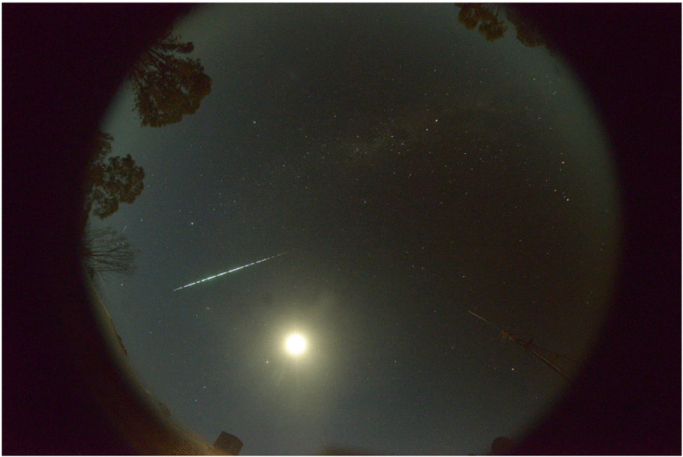
Figure 1. Camera image showing a 3 s fireball seen relatively closely to the camera, at Perenjori in Western Australia, on 2015 April 27. Such an event is easy to detect, although extra false positive coordinates were produced due to the presence of moon and moon halo close to track.
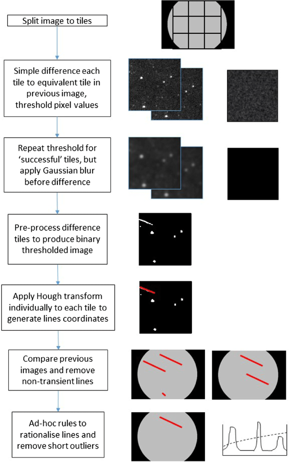
Figure 2. DFN data pipeline showing processing steps and decisions for the traditional Hough transform-based processing.
The system takes still images and the fireballs we wish to detect within them are transient phenomena. The initial operation in the chain of elimination is to calculate the difference between the current and previous image tiles and quantify any changes seen.
Step (1): We begin by calculating a brightness difference between each pixel in the tile and its corresponding pixel in the previous image’s tile and counting the number pixels that have a difference above a threshold value. The use of a threshold of difference allows small variations in brightness due to slight atmospheric or sensor issues to be accounted for. Counting numbers of anomalous pixels rather than summing their differences prevents any one anomalous pixel change to dominate the result. If no or few pixels are changed by less than a given amount, then the tile can be discarded immediately. Tiles containing the moon are essentially saturated, due to the high camera sensitivity settings, and as such will immediately fail the first difference operation, and not be passed to subsequent operations.
Step (2): This differencing operation is then repeated, but with a Gaussian blur applied independently to the current and previous tile prior to differencing. This blur operation smears objects that have moved slightly, such as stars far from the celestial pole, reducing the differenced values around such objects below the detection threshold. Tiles that drop below this blurred threshold are then discarded.
Step (3): The remaining few tiles with significant differences between current and previous are then analysed using a Hough transform (Duda & Hart Reference Duda and Hart1972) to detect straight lines in the tile and extract the pixel coordinates of any line. Specifically, we apply the progressive probabilistic Hough transform as implemented in OpenCV v2.4, ‘cv2.houghlinesP()’ (Matas, Galambos, & Kittler Reference Matas, Galambos and Kittler2000). The probabilistic transform is generally less resource-intensive than the standard transform; however, it requires a binary thresholded image. Additionally in the OpenCV implementation, the output of the function is a coordinate pair of start and end points of a line. In fact, this output is ideal for later processing steps that involve conversion from image pixels to spatial coordinates such as altitude, azimuth. To apply the probabilistic Hough transform, thus involves pre-processing and thresholding according to the following processes:
(i) Absolute difference between current and previous tiles.
(ii) The probabilistic Hough transform as implemented in OpenCV requires a binary image, so an Otsu threshold (Otsu Reference Otsu1979) is used to convert the greyscale difference to binary. The Otsu algorithm chooses a threshold based on attempting to fit two Gaussian brightness populations to the brightness histogram of the image tile. The Otsu thresholding is well suited to images containing star fields and fireballs, which essentially consist of bright points (and a bright fireball) and a dark background.
(iii) Applying a skeletonise function to reduce blurry, smeared lines (due to lens defects) down to single pixel lines, giving the Hough transform sharper edged lines to work with. Short false lines such as smeared stars are reduced to single points and not detected by the subsequent Hough transform.
(iv) A 3-pixel dilate is then applied to the skeletonised line to thicken the lines, such that the Hough transform will easily detect lines without having to finely tune the Hough voting parameters.
The progressive probabilistic Hough transform function can then be applied at a relatively high sensitivity setting, which becomes more computationally expensive as more pixels have to be checked for each putative line. But this is acceptable as only a few tiles are to be analysed. Hough parameters are chosen based on the ability of the transform to detect both dashes and long lines (in the DFN systems, the cycling of a liquid crystal shutter is used to break the fireball track into countable dashes to provide velocity data Howie et al. Reference Howie, Paxman, Bland, Towner, Cupak, Sansom and Devillepoix2017a).
Step (5): Following this line detection, a series of ad hoc rules are applied to reduce the false positives within the lists of lines detected. These rules are based around the physical expectations of likely fireball events. By applying a series of simple rules, one after the other, many false positives are removed at little computational expense:
(i) Pixel brightness is considered along the length of the line; it should be relatively constant or peaking at the line centre. A short line with high variance, with brightness peaks at line ends, will correspond to a false line fitting through two very close bright stars and is discarded. However, care must be taken in the choice of variance thresholding, to ensure that dashed lines are not discarded. Additionally, within a tile, a search is carried out for lines that are very similar (similar start and points) to remove double counting and duplicates.
(ii) The line coordinates from all tiles in one image are then collated together and filtered based on plausibility checking of the resultant list. If there is just one very short line in the whole image, for example, five pixels long or less, it is discarded as a false positive. (In reality, this could represent a fireball, but of too small or distant a result to be useful for meteorite recovery or orbit determination). Stationary or slow-moving objects are also removed, based on coordinate listings from earlier images in the sequence. Objects that appear in the same spot or moving slowly and linearly (e.g. a plane or the International Space Station) over three or more images have persisted for too long to be a fireball and are discarded or catalogued separately.
(iii) Finally, (at the single-camera level) ad hoc rules based on experience with specific problem are applied: in some cases, the Hough transforms return large numbers of lines for a single image (e.g. on a partially cloudy night, detecting cloud edges); hence, results are discarded if over 10 000 lines are observed in 1 tile. This has had the side effect of sometimes discarding the oversaturated middle sections of particularly large fireballs, but the fainter beginning and end of a fireball are still correctly detected (which is acceptable from a fireball detection and triangulation emphasis). Other issues are caused by cloud edges when they move between subsequent images as they are detected by the Hough transform as linear features. Many can be removed, as they are often persistent over multiple images, and the direction of the line detected is not the same as the direction of the apparent motion of the line between images, as would be the case for a fireball.
This process is intended to efficiently detect as many real events as possible and not miss any reasonable candidates. As such, it still generates significant numbers of false positives. From the DFN fireball point of view, this is acceptable, as it is better to have 10 false events rather than 1 important event missed.
2.1.1 Testing and evaluation datasets
For investigating the Hough transform algorithm and selecting optimum parameters, we have assembled a selection of 50 image sets to cover most plausible scenarios, as a testing dataset. These included genuine fireballs and likely false positives of a variety of sizes such as planes and satellite flares, over a variety of cloudy and clear nights, plus nights with no fireballs present (moonless and with full moon) and situations such as a bright star rising/setting, or passing behind an obscuring tree (and hence flickering between images). Examples of some of these are shown in Figure 3. This small dataset was used for the Hough transform approach for the investigation of possible parameters and was separated from the larger evaluation dataset described later in Section 3 that was used for performance evaluation of the algorithms.
The Hough transform is designed for finding linear features, such as fireballs, but the parameters must be chosen carefully to optimise for the character of the lines desired (typically length, thickness, ‘straightness’, permitted length of breaks in line), and this dataset allowed us first to test procedural changes, such as adding more filtering steps, and secondly to refine the chosen parameters. Multiple simple tests on this small dataset allowed convergence on Hough parameters as listed in Table 1. It was found that the behaviour of each parameter is relatively independent, such that inspection of the results of each test made it obvious what to change, for example, if short fireball lines were missed, alteration of the minimum line length parameter, making it relatively easy to manually optimise the Hough algorithm.
The parameters used in the algorithms were adjusted until all features were correctly identified (or discarded) in the small test dataset. Evaluation of the performance of the algorithm and parameters is described in Section 3.
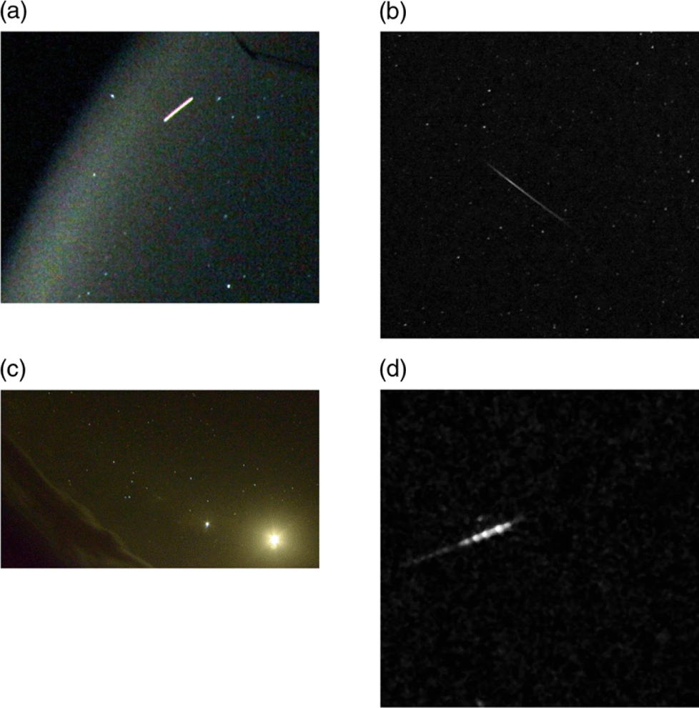
Figure 3. Testing dataset example images showing (a) plane streak, (b) satellite streak, (c) straight cloud edge and Moon aperture diffraction spikes, and (d) small fireball.
Table 1. A list of software parameters for the event detection algorithm, as detailed in the processing steps text and figure.

2.2 Neural network-based detection method
2.2.1 Pre-processing
The dimensions of the images captured by the DFN cameras are  $7360 \times 4912$
pixels; the Bayer filter in the camera means that in the raw data, 1/2 of these are green, and 1/4 each blue and red pixels. A JPEG image derived from this raw image is interpolated, to generate 36 152 320 pixels for each colour channel. Any machine learning algorithm would struggle with a vector of this size, so the image was initially split to extract only the green channel (as is also done for the traditional processing). As in the traditional processing, to make the problem more manageable, the image is then split into tiles and those tiles are classified. A tile size of
$7360 \times 4912$
pixels; the Bayer filter in the camera means that in the raw data, 1/2 of these are green, and 1/4 each blue and red pixels. A JPEG image derived from this raw image is interpolated, to generate 36 152 320 pixels for each colour channel. Any machine learning algorithm would struggle with a vector of this size, so the image was initially split to extract only the green channel (as is also done for the traditional processing). As in the traditional processing, to make the problem more manageable, the image is then split into tiles and those tiles are classified. A tile size of  $25 \times 25$
pixels gives a state vector of length 625, which is suitable for a simple neural network classifier. However, a tile of this size is a very small part of the sky, typically less than one degree of viewing angle. Hence, to ensure that 25 × 25 is a large enough area of the image to encompass reasonable features—such as fireball streak—before tile generation, the image was down-sampled by factor 2 using bilinear interpolation. Hence, the tile now represents approximately 2 × 2 degrees, albeit at a lower resolution, which better supports the software goal of detection of bright fireballs in a tile, not precise position of that fireball.
$25 \times 25$
pixels gives a state vector of length 625, which is suitable for a simple neural network classifier. However, a tile of this size is a very small part of the sky, typically less than one degree of viewing angle. Hence, to ensure that 25 × 25 is a large enough area of the image to encompass reasonable features—such as fireball streak—before tile generation, the image was down-sampled by factor 2 using bilinear interpolation. Hence, the tile now represents approximately 2 × 2 degrees, albeit at a lower resolution, which better supports the software goal of detection of bright fireballs in a tile, not precise position of that fireball.
For the neural network classifier, as in the traditional processing, pre-processing significantly improves the true positive rate. In particular, reducing the image background noise reduces spurious detections. However, thresholding was done in a slightly more complex manner to the approach above; the previous image was blurred and subtracted from the current image, and then reciprocally the current image was blurred and subtracted from the previous image. Binary dilation was applied independently to each image of the new pair, before the two images were compared. This process effectively allows for changes in background brightness between images (such as closer to sunrise/set) and also blurs out and removes star edges (which may have shifted slightly between images), preventing them from generating false positives, leaving only major differences. Compared to the Hough transform approach, this highlights changes more, at the expense of line precision, which is better suited to a tile classifier compared to a line detector.
Another benefit of this approach to image subtraction and filtering was to address a few issues encountered by the traditional detection code. It was noticed that features such as three close stars linearly arranged would often produce a false positive identification, interpreted as three dashes of the fast meteor streak. This was particularly an issue with stars far from the celestial pole, such that there was a significant movement between frames, so that basic image differencing was imperfectly removing those leaving residual peaks that were misinterpreted.
2.3 Neural network details
By breaking the original image into 25 × 25 pixel tiles, this generates an input vector to the neural network of 625 integers. The network requires one output unit, giving a 0 or 1 for a tile, of ‘fireball’ versus ‘non-fireball’.
It was decided to code the neural network in Python, rather than using one of the existing implementations, to give more control over minimising resource use on a camera system. A single-layer, forward propagating neural network was constructed with a gradient descent optimisation minimise function (from SciPy Virtanen et al. Reference Virtanen2019), with back propagation explicitly implemented in training.
The choice of the optimal number of hidden layers and nodes in a neural network for a particular task is currently not an analytically solved problem and is usually approached heuristically. Conventionally, the number of hidden nodes should be between the number of output and input units—so from 1 to 625— and ideally it is dependent on the number of training examples (Nielsen Reference Nielsen2015). We have carried out an initial investigation and testing using a training dataset (detailed below) to test performance versus computation time over the range of 1–10 hidden nodes. Under five hidden nodes, the network was suffering from high bias, as the model could never reach a higher accuracy than 70% on the training set. Above five hidden nodes, the difference in the outcome was so small that it was difficult to choose the best parameter. Above 10 hidden nodes, issues arose due to excessive time and computational requirements. Hence, 10 hidden nodes seemed reasonable to achieve high performance without considerably suffering from high variance. In the case of this binary classifier, we have used the SoftMax cross-entropy cost function, with gradient descent (Nielsen Reference Nielsen2015).
Within the overarching pipeline—similar to the traditional processing pipeline—ad hoc post-processing operations helped to improve the algorithm success rate. The tiles were classified by the network into fireball or non-fireball, and results for each image were collated, and coordinates were processed in identical manner to the Hough transform-based detection, such that slow-moving objects seen in three consecutive images were ignored. Coordinates for the fireballs seen are represented as centre of fireball-classified tiles and so are accurate to 25 pixels. This is not as precise as the Hough technique (resulting in typically  $2^\circ$
of altitude/azimuth pointing accuracy) but good enough for a central server to carry out preliminary triangulations to check for the validity of proposed trajectory.
$2^\circ$
of altitude/azimuth pointing accuracy) but good enough for a central server to carry out preliminary triangulations to check for the validity of proposed trajectory.
2.4 Neural network training and test dataset
Successful learning of a neural network is achieved by the quality and quantity of the materials provided to the network along with the right parameter selection. When dealing with numerous features, the datasets are usually partitioned in three parts: the training, cross-validation, and test dataset. These sets are strictly independent from each other but made of similar examples that could have been used for any set. The three datasets (separate to the Hough transform dataset discussed earlier) were initially prepared by collecting some examples from manually searching the images. About 50 images of manually selected fireball events were pre-filtered giving 200 tiles containing fireball streaks. The same quantity of negative examples were obtained from noisy images containing background noise or unidentifiable parts of meteor streaks, some examples of which are shown in Figure 4. Training based on this dataset showed that the cost function had not fully stabilised. Hence, all three datasets were expanded by factor of 8, by duplicating and then flipping and/or rotating each example tile. The three datasets were then made of an equal proportion of positive and negative samples randomly distributed to each dataset with 60% to the training set, 20% to the cross-validation set, and 20% to the test set. In Section 3, more detailed comparison of the algorithm’s performance is carried out using a large evaluation dataset.

Figure 4. Examples of positive fireball samples (left group of six images) and negative samples (right) for neural network training.

Figure 5. Receiver operating characteristics plot for the neural network for all training and validation data combined.
Figure 5 shows the receiver operating characteristics for the trained network, using the validation dataset. The area under the curve indicates that the cross-entropy function is successfully discriminating fireballs, within this dataset. Stabilisation of the cost function after training indicated that training had plateaued. The confusion matrix results for training, validation, and test sets were all 92.8%  $\pm$
0.6 success for true positives, with final detection success values for whole images as discussed in the next section.
$\pm$
0.6 success for true positives, with final detection success values for whole images as discussed in the next section.
3. Event detection testing results and discussion
All testing and evaluation of the algorithms were carried out on the identical hardware as deployed in the DFN cameras, but in a laboratory setting using stored images that had been collected in the field by camera prototypes. The algorithm must be able to process a full night’s worth of images during the day to keep up with the data volumes generated. Initial testing showed this was not a major concern for all plausible variations on the algorithms. Typically, the average processing time for an image was 6 s for the traditional approach and 5 s for the neural network, resulting in processing a full night’s data in about 2 h.
To test the performance of the on-board camera detection procedures, a month of real observations from one fireball camera (24 457 images) was surveyed manually for fireballs, and these observations were then compared to results using the traditional and neural network event detection procedures.
Table 2. Analysis of 5 weeks of imagery from a single camera, in blocks of 5d, from late 2015. Columns describe the results of the Hough transform-based algorithm and the neural network algorithm, as compared to a manual analysis which provides a control dataset.

Table 3. Data subdivided into long/big fireballs and remainder (‘small fireballs’). Long/big fireballs are defined as greater than one Hough size image tile (400 × 400 pixels).

Details of the manual and automated testing results for the month’s data are shown in Tables 2 and 3. The data appear as seven rows showing groupings of five nights of observations, to indicate the variability seen. Summary statistics are shown at the base of the table. Some five night groups, such as the 11-15 block—starting on 2014 November 15—have relatively few images present, showing several fully or partially cloudy nights of observations. During cloudy nights, the camera system takes fewer images to minimise unnecessary data storage. In both the manual surveying and software-based detection, satellites are counted as valid events equivalent to a fireball and no distinction is made: satellite streaks are valid events from the point of view of a single camera, and detection and triangulation of satellites remains a relevant scientific interest for the camera network, in addition to the primary goal of meteorite recovery and orbit determination. From the Table 2 summary, for all fireballs the algorithmic detections have a success rate of about 70% compared to manual surveying. This at first appears less than ideal, given the high priority of avoiding true negatives at the expense of false positives. However, the manual surveying is recording all fireballs, from the very smallest seen by the eye upwards [see, e.g. Figure 6(a)]. Given that the overarching rationale for the fireball detection is to recover meteorites, the software’s ‘goal’ is to highlight large fireballs. Therefore, to investigate this further in the data table, we also highlight large fireballs only. Large is defined as appearing on two or more adjacent tiles or having a brightness that is saturating the sensor at the brightest spot, for example, Figure 6(b) and (c). In this case, the automated true positive rate is about 96% Hough/100% Neural, more in line with the project requirements. Of the 51 large fireballs observed, the traditional software missed two: they were both long streaks from satellite traces, where the length resulted in a large classification. However, the brightness of the trace was relatively low, which resulted in a failure to highlight the streak at the Otsu thresholding stage [Figure 6(d)]. The neural network version detected all large fireballs. As a brief trial to investigate the traditional algorithm, it was found that increasing this testing dataset did not improve success rate; we feel this is likely a consequence of the pure variability of possible fireball streaks, with the shape, brightness, fragmentation such that it is difficult to derive a set of Hough parameters to cover all contingencies.
In Table 2, the 5-night group 11–25 to 11–30 has high number of false positives (278 for the Hough algorithm and 1560 for the neural network). On the night of November 29, there was a thunderstorm on the horizon, which resulted in lightning repeatedly illuminating the edges of distant clouds producing transient bright lines on the image, which was erroneously flagged as events by the software [Figure 6(e)], as they satisfy the criteria of a single ‘straight’ line, with constant brightness along the line, and nothing in the prior and subsequent images. This produced over 70 false positives in one 3 h period. Fortunately, this combination of straight cloud edge near the horizon with internal lightning appears relatively infrequently, as closer storms would not give the same appearance. As described in later sections, such events are filtered from the data pipeline at the camera-to-camera triangulation stage of analysis.
False positives from the on-board camera detection algorithm appear overall at the rate of approximately 4 times the real events for the Hough algorithm, but approximately 10 times for the NN. Other examples of false positives are beams of light from camera internal reflections and cloud edges as previously discussed. Table 4 shows the confusion matrix for the two algorithms to gauge their efficacy. This highlights the result that the neural network is marginally better at detecting fireballs, but at the expense of false positives. To investigate this, Table 3 separates fireball detections into large and small fireballs (a large fireball being defined as one that occurs over multiple tiles in the detection algorithm). It is clear that both algorithms are successful at larger fireballs, with the neural network better for the smaller fireballs. In the case of the Hough transform, this could be due to the use of the Otsu threshold, such that faint fireballs do not fall below the threshold. The large number of false positives for the neural network indicates a possible problem with the training dataset. The negative examples in the training dataset include many tiles of static stars, which would be the primary-type negative tile that the algorithm would encounter in routine operations. However, the other negatives would be transient true negatives, such as lens flares or internal reflections, moonbeam, and other artefacts, which would occur in many possible orientations and configurations. Given the larger image archive now available from the fully operational DFN, this dataset could be extended.
Almost all of these false positives are discarded at the camera-to-camera level, as they fail to match with a corresponding event on an adjacent system. Satellite observations as opposed to genuine fireballs are of interest for a variety of studies. They can be separated from fireball event alerts from calculation at the multiple camera level, whereby triangulation of the data will indicate the altitude and orbit of the object (also allowing removal of low level objects such as planes).
Several known false positive scenarios will be passed by the single-camera event detection: imagery of aeroplanes usually lasts more than 30 s, stretching over three images, and are thus easy to filter. This will not discard a small satellite flare or plane that lasts less than 30 s.
4. Overall initial event detection rates
We can briefly estimate the efficiency of the network as a whole for detection, using single-camera estimates as a basis. For the detection of a fireball in a two-camera network, each detecting independently, the probability of detection is P(A)  $\times$
P(B), where P(X) is the probability of fireball detected at camera X. In the simplest case P(A) = P(B), and for large fireballs P(A) is 0.958 (Hough) or 1.0 (NN) from Table 3, giving two-camera fireball detection as
$\times$
P(B), where P(X) is the probability of fireball detected at camera X. In the simplest case P(A) = P(B), and for large fireballs P(A) is 0.958 (Hough) or 1.0 (NN) from Table 3, giving two-camera fireball detection as  $P(A)^2$ $\approx$
0.92 or 1.0.
$\approx$
0.92 or 1.0.
Table 4. Confusion matrix from evaluation of the Hough and neural network algorithms on the 5-week collection of imagery as described in main text and previous tables.

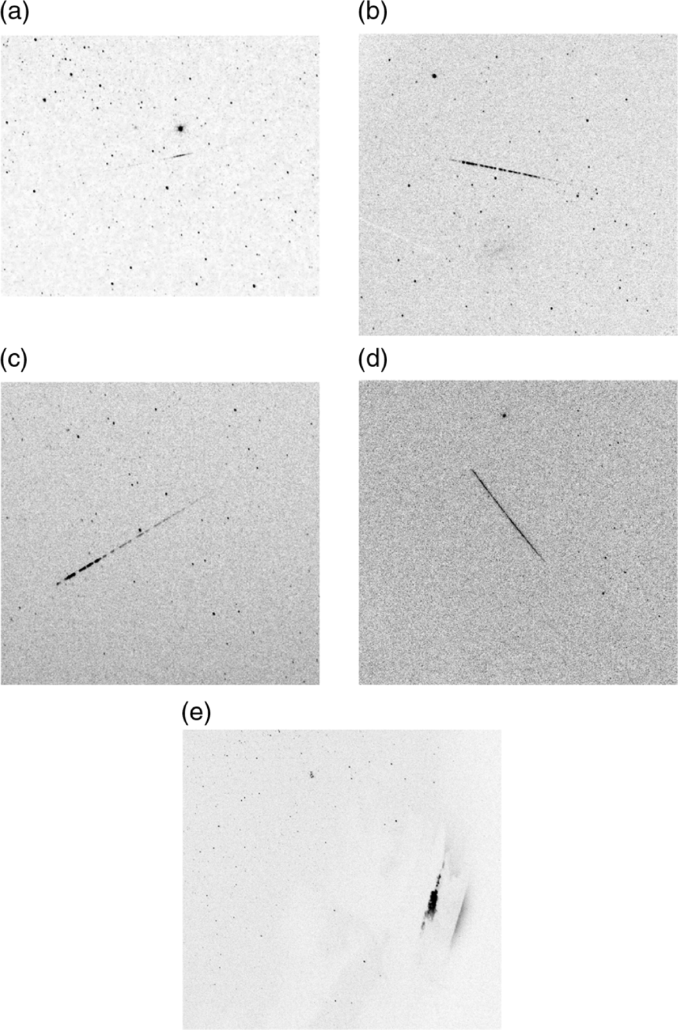
Figure 6. Results of the autodetection algorithms (Hough and NN), showing examples of a variety of small fireballs and false alarms. (a) small fireball not observed by autodetection, (b), (c) fireballs detected by autodetection, (d) one of the two ‘large fireballs’ not seen by Hough-based detection algorithm (actually a relatively dim satellite streak), and (e) lightning-illuminated cloud on the horizon that produced a false positive. For clarity to the reader, the images have been inverted, to black on white, rather than what would normally be a white streak on a black background. In reality, the algorithm processes the raw white on black image.
However, the reality of more cameras means that fireballs are rarely (only in literal network edge cases) going to appear on only two cameras, and viewing distance and conditions will break the equality. We can illustrate this with consideration of two examples: in the case of four cameras in a square, with a fireball in the middle, the probability to successfully detect a fireball pair becomes one minus the probability of all cameras failing to detect the event, plus the possibility of four combinations of three cameras failing to detect the event (such any two cameras detecting the event will count as successful result). Where the failure of a camera to detect an event is  $1-P(A)$
, so this calculates explicitly as:
$1-P(A)$
, so this calculates explicitly as:
 \begin{equation}1-[(1-P(A))^4+4(1-P(A))^3],\end{equation}
which evaluates to 0.9997 (Hough) and 1.0 (NN) with the values above.

Figure 7. A sketch diagram of the idealised ground layout of camera network in a triangular pattern, with two central primary cameras (solid circle) and surrounding secondary cameras (open circle).
In the second illustrative example, we can consider the hypothetical case of a triangular pattern camera network, such as shown in Figure 7. The two ‘primary’ cameras (A) close to fireball give a probability of P(A) each, and surrounding secondary cameras (a) would have a lower detection efficiency due to the greater distance of the fireball event (denoted P(a)). A successful triangulation occurs when any two cameras detect the event. So the detection success of the array can be estimated as a one minus the combinations of failures-to-detect from the two primary cameras and eight secondary cameras. For two primary and N secondary, we write P(2Pf,  ${N}-1$
) as the probability of both primaries failing and
${N}-1$
) as the probability of both primaries failing and  ${N}-1$
secondaries failing, and similarly P(1Pf, N) is the probability of one primary failing and all secondaries failing. These can be evaluated as:
${N}-1$
secondaries failing, and similarly P(1Pf, N) is the probability of one primary failing and all secondaries failing. These can be evaluated as:
 \begin{align}
P(2{\rm Pf},N-1) &= (1-P(A))^2.N(1-P(a))^{N-1}\nonumber\\
P(1{\rm Pf},N) &= (1-P(A).(1-P(a))^N
\end{align}
\begin{align}
P(2{\rm Pf},N-1) &= (1-P(A))^2.N(1-P(a))^{N-1}\nonumber\\
P(1{\rm Pf},N) &= (1-P(A).(1-P(a))^N
\end{align}
Giving:
 \begin{align}
P({\rm successful}\> & \ {\rm triangulation}) = \nonumber\\ & 1 - [P(2{\rm Pf},N-1) + P({\rm Pf},N)]\end{align}
\begin{align}
P({\rm successful}\> & \ {\rm triangulation}) = \nonumber\\ & 1 - [P(2{\rm Pf},N-1) + P({\rm Pf},N)]\end{align}
Using the small fireball detection estimate from Table 3 of 0.66 (Hough) and 0.82 (NN), we can estimate (3) as 0.997 (Hough) and 0.99995 (NN). In this network configuration, there is also the network edge case, where the fireball is outside the centre of the network and seen close to two cameras and more distantly by the surrounding five cameras. In this case, (3) gives the probability of success as 0.94 (Hough) and 0.995 (NN). In these simple illustrative calculations, we can see that despite a lower small fireball detection threshold for individual systems, the advantage of many combinations of cameras results in a high-network triangulation reliability. Note this is only the theoretical detection rate when the cameras are operating: to calculate the full true detection rate of the network in order to derive an Earth fireball flux, consideration must be made of cloud coverage, twilight, Moon saturation, operational failures, brightness, and distance from observatories, as discussed in detail in Halliday et al. (Reference Halliday, Blackwell and Griffin1989) and Ceplecha (Reference Ceplecha1992) with reference to prior camera networks. From the point of view of a network orientated towards meteorite recovery, the detection priority will be the larger, brighter fireballs, regardless of the detection rate for smaller fireballs.
5. Processing pipeline of event data
The single-camera event detection algorithms uncover possible fireballs, including any false positives. Based on the values in Table 2 for a single camera, we could estimate the total number of events for a reasonable network—say 50 cameras—to see that it is implausibly large for human checking and classification. Hence, there is a requirement for a cost-effective large network to automate as much of the remaining data pipeline as possible, with the final goal being a high-quality dataset of confirmed, genuine fireballs with analysis giving mass, velocity, and orbit (and fall position if there is a meteorite fall). To do this, one must remove the remaining false positives and then analyse the full-resolution images of the genuine fireballs.
Following the single-camera event detection, the first step in this chain is to process the events seen on each system converting from (pixel x, y, time) coordinates to astronomical coordinates (altitude, azimuth, time) using a predetermined calibration function and then transferred as simple text files to the DFN central server, which then collates events, looking for multiple camera observations of each possible fireball.
5.1 Triangulation
To search for correlations between single-camera events, the DFN central server initially iterates through each camera, each event seen and attempts to match with other contemporaneous events on other cameras based on time and locality (typically within 500 km). These coincident pairs at then triangulated, using the method of planes technique described by Ceplecha (Reference Ceplecha1987), which is purely geometrical and includes no fireball velocity/timing analysis. Triangulations using intersection of planes will always produce a solution, as the planes will always intersect unless they are parallel, but the resulting solution may be unphysical. So results can be triaged to remove implausible results—such as intersection of planes below the surface of the Earth or beyond the orbit of the moon. By a further choice of thresholds, it is possible to separate out events that are physical but too high, in the case of satellites, or too low, in the case of aeroplanes (although aeroplanes are so low that they are unlikely to be seen on multiple cameras that are many kilometre apart). The resulting events consist of approximate fits to the meteor path, with no timing information.
5.2 Manual review of valid triangulations
Following successful triangulation as part of main data processing pipeline, preview images and coordinate data for any successful triangulations are sent by email for review by a team member. This human review acts as a quality check on the dataset and will remove special cases of spurious false positives, such as coincidental lucky geometries, where a false positive on two cameras will successfully triangulate to produce a valid geometry. Due to the prior filtering steps, this human interaction is not too onerous in terms of time; typically, the authors handle 5–10 emails/d for a 50-camera network, of which 1–2 are genuine events. Each email can be quickly scanned to check visually that the preview images show a fireball, and that the latitude, longitude, height, geometry is sensible. Valid results are added to the DFN consolidated dataset as genuine fireballs, where more detailed characterisation is performed.
5.3 Automatic download of full images, precise calibration
Prior to this step, validation and initial triangulation of an event was using lower resolution versions of the images, for data bandwidth and computational speed reasons. After validation, these events are fewer in number, so can be analysed in detail; the full-resolution raw images are automatically collected from the cameras, along with a full-resolution calibration image. The calibration image is processed to accurately measure the pixel to altitude–azimuth conversion function for the camera at that particular time and location. This is done using specialist software developed in-house: the image is first converted to FITS format (Hanisch et al. Reference Hanisch, Farris, Greisen, Pence, Schlesinger, Teuben, Thompson and Warnock2001) and de-Bayered to remove the Bayer colour filter pattern within the camera sensor. Star positions in the image are extracted using Sextractor tool (Bertin & Arnouts Reference Bertin and Arnouts1996), and star patterns are matched to the ACT star catalogue (Urban, Corbin, & Wycoff Reference Urban, Corbin and Wycoff1998) to produce a polynomial function that maps pixel to altitude–azimuth.
5.4 Picking of event timing
The DFN cameras record still images using a DSLR, typically 25 s exposures. To encode timing information into the fireball streak, the system includes a liquid crystal shutter in the lens, which is flickered with a known pattern to encode timing information into a fireball streak, as detailed in Howie et al. (Reference Howie, Paxman, Bland, Towner, Cupak, Sansom and Devillepoix2017a). This encodes absolute timing into the fireball streak, but this pattern must be decoded, and to date this can only be done by human interaction and pattern matching. There are complexities such as meteor fragmentation, flaring, or break-up that make this task currently a challenging problem for computer vision. Hence, within the pipeline, this final human interaction step is the precise marking of dashes for the fireball track to accurately timestamp each dash.
To do this, the DFN project developed a helper tool that provides a graphical user interface (GUI) to allow easy marking of fireball streaks using mouse clicks on an image. This is the most human time-intensive part of the pipeline, as each image can take approximately 5 min to analyse fully, and there are multiple images per event.
5.5 Automated precise triangulation, generation of an orbital dataset
The fully calibrated dataset including time information for each fireball is now sufficient to process fully the event automatically, producing final orbit results, and if reasonable, predicted fall positions of any putative meteorite. The triangulation calculation is now redone, using the straight-line-least-squares method (Borovicka Reference Borovicka1990) and a 3D particle filter method (Sansom et al. Reference Sansom, Bland, Paxman and Towner2015), to give precise trajectory, and hence orbital parameters (Jansen-Sturgeon, Sansom, & Bland Reference Jansen-Sturgeon, Sansom and Bland2019). Fireball mass estimates are generated from the dynamic data (Gritsevich et al. Reference Gritsevich2017). Errors are propagated in all parameters using a Montecarlo framework. This gives an automatically generated, consolidated dataset of all significant fireballs seen by the network, with associated orbits. Team members can easily review this at top level, highlight any issues, and focus on more in-depth processing of the most promising meteorite-dropping candidates.
5.6 Human detailed review of potential meteorite droppers
One goal of the DFN is meteorite recovery, and conducting a ground search with multiple personnel of a remote area in Australia is a significant and costly exercise. Hence, where analysis predicts that a fireball has dropped a meteorite, the full dataset for the event is manually reviewed. Additionally further processing is needed, as discussed in outline, for example, in Spurný et al. (Reference Spurný2012) and Devillepoix et al. (Reference Devillepoix2018): a wind profile is calculated using a global climate model (WRF v3, Skamarock et al. Reference Skamarock2008) giving the atmospheric parameters as a function of height at the specific fall site. This knowledge is required for ground fall predictions, as wind and pressure effects will result in the meteorite falling up to several kilometres away from the idealised, still-atmosphere case. Darkflight modelling is carried out as a simple integrator of an object in free fall, with a montecarlo propagation of possible shapes/mass ranges/rock density ranges (Spurný et al. Reference Spurný2012), to give a predicted fall search area, which is then used to plan ground searching activities.
6. Conclusions
The DFN consists of an array of remote astronomy camera systems in the Australian outback designed to observe and detect incoming fireballs, with the goals of (1) recovering meteorites and (2) generating a statistically significant fireball orbital dataset. The observatory cameras are constrained by electrical and computing power, in order to maximise ground coverage per unit cost, and hence maximise meteorite recovery chances. Additionally, the network is also constrained by a relatively small team size, forcing the implementation of an automated data pipeline with minimal routine human interaction.
Since the cameras are operating remotely and independently, the images collected during a night must be processed on-board for the detection of fireball trails. We have developed an image processing chain intended for small power systems, whereby a cascading series of more computationally expensive operations are applied to smaller and smaller regions of interest. We implement this as a tool chain of initially simple operations like subtraction or Gaussian blur, followed by a Hough transform. Supplementary ad hoc rules to remove objects, like slow-moving planes, reduce the number of false positives. In parallel, for comparison, we have also implemented a simple neural network approach, based on a single-layer forward propagator with a hidden layer of 10 nodes, again with pre-processing to improve success rates and ad hoc post-processing to remove some false positives. Both the Hough transform-based approach and the neural network approach are capable of processing a full night’s data within a few hours on the DFN hardware, allowing the operations to keep up with the incoming data. The currently deployed PC is a Commell LE-37D with an Atom N2930 1.83 GHz processor, handling a night of typically 1000 images of 36 megapixel each from a Nikon D810 DSLR (Howie et al. Reference Howie, Paxman, Bland, Towner, Cupak, Sansom and Devillepoix2017b).
In a facility such as the DFN, where important scientific events—meteorite falls—are rare and random, the primary metric of an automated detection algorithm is to minimise the false negatives. False positives are acceptable, until such point as they swamp true positives in the operations. However, by processing the imagery on the remote camera system, and only returning streak coordinates, the threshold for practical handling of false positives is high. Testing of both the Hough transform and neural network approaches using a evaluation dataset of raw data collected over 1 month of operations indicates that both approaches are an efficient method for use in situations of constrained computing, such as low-power equipment. The traditional method was slightly less effective than the neural network particularly at detecting smaller/fainter fireballs, although the neural network generates significantly more false positives without sacrificing true positives, giving a large fireball, single-camera event detection rate of 96% compared to manual observations of data. (Increased size of the training dataset for the neural network did not mitigate this rate of false positives, so it does not appear to be an under-training issue.) Both the traditional and neural network processing are most effective with larger fireballs (defined as appearing on multiple tiles in the image detection algorithm), but have a lower success rate with smaller, fainter meteors. However, the topology of the camera network means that several cameras have the opportunity to observe an event, so even a mediocre rate for single-camera small fireball cases still results in a high-network fireball detection rate across the network, such that the critical metric for meteorite recovery is that the detection rate is better than 99.9% for large fireballs. Consequently, since the network topology mitigates the risk of missing large fireballs, we have currently favoured the Hough transform algorithm within the DFN due to the lower number of false positives it generates (since the DFN is a relatively large network with over 50 cameras currently). The Hough transform detection also has the advantage of giving precise line coordinates for the fireball seen, whereas the neural network merely gives the tile coordinates for a 25 × 25 pixel tile classified as containing a fireball. This extra information improves the precision of preliminary triangulations as described in Section 5.1, screening out more non-meteoritic events such as aeroplanes. However, both approaches appear to work well and would be effective for the primary goal of meteorite recovery.
To handle the large volumes of events generated by a digital camera network, an automated pipeline was constructed for routine processing of fireball data. Data processing has focused on correctly identifying all large fireballs capable of dropping meteorites. This high initial fireball detection rate comes at the expense of generating false positive events, and the later data pipeline processing is designed to remove the majority of these automatically, before human intervention to verify remaining true positives. This human discrimination is done using image thumbnails and lower resolution copies of the raw data, minimising bandwidth and computational time. Single-camera event detection is followed by server-level triangulation allowing filtering of non-fireball geometries, followed by human checking of the fireball validity, via alert emails. Post-verification, the full-resolution images are downloaded from cameras automatically, calibrated using star positions, and the fireball streaks must be tagged by a human to add fireball time/velocity information (due to the computational difficulty of automated image processing to distinguish fireball fragmentation, flares, etc.). Finally, derived data can then be processed to estimate meteor parameters. The resulting dataset is a combined total of genuine fireballs with trajectory and orbital parameters, and, if an object survives, predicted meteorite mass and fall position.
Automation of much of the routine processing steps allows a large camera network to be run with relatively little human supervision, allowing the construction of larger network than would have been possible in the past before the advent of digital technology.
Acknowledgements
This research was supported by the Australian Research Council through the Australian Laureate Fellowships scheme and receives institutional support from Curtin University.


