


1. Introduction
Rotating Radio Transients (RRATs) represent a relatively new class of pulsar, primarily characterised by their sporadic bursting emission of single pulses on time scales of minutes to hours. In addition to the difficulty involved in detecting these.
Rotating Radio Transients (RRATs) are a relatively new population of pulsar that were discovered after reprocessing of the Parkes Multibeam Pulsar Survey for single-pulse events (McLaughlin et al. Reference McLaughlin2006). They are characterised by sporadic emission of individual pulses, where a single pulse is detected followed by no detectable emission for many rotations (sometimes minutes to hours). RRATs are almost certainly Galactic neutron stars with extreme emission variability (e.g. McLaughlin et al. Reference McLaughlin2006, Reference McLaughlin2009; Keane et al. Reference Keane, Kramer, Lyne, Stappers and McLaughlin2011; Keane Reference Keane2016; Bhattacharyya et al. Reference Bhattacharyya2018). Based on objects with adequate observations, we expect single-pulse rates in the range of a few pulses to a few hundred pulses per hour. RRATs are therefore more easily detected through single-pulse searches as opposed to the standard Fourier domain search or traditional folding techniques. Even though there are 111 known RRATs,a the inherent difficulty in their detection has meant that the physics responsible for the sporadic nature of the emission remains unclear.
The pulsar and magnetosphere system geometries are thought to play a vital role in the characteristics of pulsar emission, and can be constrained through polarisation measurements (e.g. Gould & Lyne Reference Gould and Lyne1998; Manchester et al. Reference Manchester, Han and Qiao1998; Weisberg et al. Reference Weisberg1999; Everett & Weisberg Reference Everett and Weisberg2001; Mitra et al. Reference Mitra, Basu, Maciesiak, Skrzypczak, Melikidze, Szary and Krzeszowski2016; Johnston & Kerr Reference Johnston and Kerr2018). For RRATs this can pose a challenge given that, in general, the folded profiles are not particularly well defined by virtue of their sporadic emission. Nevertheless, when the polarisation properties have been analysed, even based on a small sample of single pulses, they provide remarkable insight into the nature of the emission (e.g. RRAT J1819−1458, Karastergiou et al. Reference Karastergiou, Hotan, van Straten, McLaughlin and Ord2009). Generally speaking, very little is known about whether the RRAT population exhibits polarisation characteristics similar to the normal pulsar population. This is, in part, due to a lack of single-pulse analysis of normal pulsars in the literature, combined with the difficulty of creating high quality polarimetric profiles of RRATs.
Several models have been proposed to explain the sporadic emission, most of which are also linked to intermittent pulsars and the nulling phenomenon. Some examples include: extreme nulling (e.g. Wang et al. Reference Wang, Manchester and Johnston2007; Burke-Spolaor & Bailes Reference Burke-Spolaor and Bailes2010), asteroidal or circumpulsar debris (Michel & Dessler Reference Michel and Dessler1981; Li Reference Li2006; Cordes & Shannon Reference Cordes and Shannon2008), or even mechanisms within the pulsar magnetosphere (e.g. Timokhin Reference Timokhin2010; Li et al. Reference Li, Spitkovsky and Tchekhovskoy2012; Melrose & Yuen Reference Melrose and Yuen2014). Studying the pulse-energy distributions (e.g. Shapiro-Albert et al. Reference Shapiro-Albert, McLaughlin and Keane2018; Mickaliger et al. Reference Mickaliger, McEwen, McLaughlin and Lorimer2018), timing periodicities and pulse clustering (e.g. Palliyaguru et al. Reference Palliyaguru2011), and flux density or pulse energy correlations with single-pulse detection statistics (e.g. Cui et al. Reference Cui, Boyles, McLaughlin and Palliyaguru2017) of RRATs is vital in understanding their emission and how they connect to the canonical pulsar population.
To further uncover connections between RRATs and normal pulsars, it is also important to understand their kinematic properties, such as space velocities and proper motions. Techniques used to do this for normal pulsars include Very Long Baseline Interferometry (VLBI) (e.g. Deller et al. Reference Deller, Weisberg, Nice and Chatterjee2018), multi-wavelength analysis of binary systems (e.g. Jennings et al. Reference Jennings, Kaplan, Chatterjee, Cordes and Deller2018), long-term precision timing experiments (e.g. Janssen et al. Reference Janssen, Stappers, Bassa, Cognard, Kramer and Theureau2010; Gonzalez et al. Reference Gonzalez2011), and scintillation analysis (e.g. Cordes Reference Cordes1986; Johnston et al. Reference Johnston, Nicastro and Koribalski1998; Bhat et al. Reference Bhat2018). None of these techniques has been applied to RRATs in order to extract the pulsar velocities, specifically. In particular cases, scintillation studies of RRATs would nominally be able to not only provide estimates of the space velocities, but also allow direct measurement of the turbulence and characteristic scales of the interstellar medium (ISM) along the respective sight-lines, thus allowing them to be used as additional probes of the structure and composition of the ISM.
RRAT J2325−0530 was originally discovered as part of the Robert C. Byrd Green Bank Telescope (GBT) 350 MHz Drift-scan pulsar survey (Boyles et al. Reference Boyles2013; Lynch et al. Reference Lynch2013). The pulsar has a pulse period of $P=0.868\,\text{s}$
, a moderate dispersion measure,
$P=0.868\,\text{s}$
, a moderate dispersion measure, $\rm DM=14.966\pm 0.007\,pc\,cm^{-3}$
, and a nominal pulse rate of
$\rm DM=14.966\pm 0.007\,pc\,cm^{-3}$
, and a nominal pulse rate of $\rm\sim\!50\,h^{-1}$
. Karako-Argaman et al. (Reference Karako-Argaman2015) conducted follow-up observations of a subset of those RRATs detected in the survey, including RRAT J2325−0530, using the GBT at 350 MHz (though with a larger bandwidth and upgraded digital backend) and the Low Frequency Array (LOFAR; van Haarlem et al. Reference van Haarlem2013; Stappers et al. Reference Stappers2011) core stations at 150 MHz. This pulsar has also been observed with the first station of the Long Wavelength Array (LWA1; Taylor et al. Reference Taylor2012) over a frequency range of 30–80 MHz (Taylor et al. Reference Taylor, Stovall, McCrackan, McLaughlin, Miller, Karako-Argaman, Dowell and Schinzel2016), allowing the measurement of a relatively shallow spectral index (
$\rm\sim\!50\,h^{-1}$
. Karako-Argaman et al. (Reference Karako-Argaman2015) conducted follow-up observations of a subset of those RRATs detected in the survey, including RRAT J2325−0530, using the GBT at 350 MHz (though with a larger bandwidth and upgraded digital backend) and the Low Frequency Array (LOFAR; van Haarlem et al. Reference van Haarlem2013; Stappers et al. Reference Stappers2011) core stations at 150 MHz. This pulsar has also been observed with the first station of the Long Wavelength Array (LWA1; Taylor et al. Reference Taylor2012) over a frequency range of 30–80 MHz (Taylor et al. Reference Taylor, Stovall, McCrackan, McLaughlin, Miller, Karako-Argaman, Dowell and Schinzel2016), allowing the measurement of a relatively shallow spectral index ( $\alpha_{30}^{80}\approx -0.7$
).
$\alpha_{30}^{80}\approx -0.7$
).
In this paper, we present simultaneous observations of single pulses from RRAT J2325−0530 with the Murchison Widefield Array (MWA) at 154 MHz and Parkes radio telescope at 1.4 GHz. RRAT J2325−0530 is also the first RRAT detected with the MWA. In Section 2, we describe the observations and calibration procedures. Section 3 presents our analysis and results, followed by discussion in Section 4. Finally, we summarise in Section 5. Throughout, we define the spectral index, $\alpha$
, by
$\alpha$
, by $S_{\nu}\propto\nu^{\alpha}$
, where
$S_{\nu}\propto\nu^{\alpha}$
, where $S_{\nu}$
is the flux density measured at frequency
$S_{\nu}$
is the flux density measured at frequency $\nu$
.
$\nu$
.
2. Observations and calibration
RRAT J2325−0530 was simultaneously observed with the MWA and Parkes radio telescope on 2017 June 27. The MWA observed with a 30.72 MHz bandwidth centred on 154.24 MHz for 1.4 h, while Parkes observed at a centre frequency of 1396 MHz with 256 MHz bandwidth for 1.6 h. Observing details are summarised in Table 1.
Table 1. Observing details for MWA and Parkes on 2017 June 27.

a Delay between the highest Parkes band and the lowest MWA band.
2.1. MWA
The MWA is a low-frequency (70–300 MHz) Square Kilometre Array (SKA) precursor telescope. Phase I of the MWA was composed of 128 tiles, each containing 16 dual-polarisation dipole antennas, distributed with a maximum baseline of $\sim\!3\,\text{km}$
(Tingay et al. Reference Tingay2013). The Phase II upgrade of the MWA, which was completed in October 2017, provides an additional 128 tiles: 76 in two redundant hexagonal configurations near the array centre, with the remaining 52 tiles facilitating maximum baselines of
$\sim\!3\,\text{km}$
(Tingay et al. Reference Tingay2013). The Phase II upgrade of the MWA, which was completed in October 2017, provides an additional 128 tiles: 76 in two redundant hexagonal configurations near the array centre, with the remaining 52 tiles facilitating maximum baselines of $\sim\!6 \ \text{km}$
(Wayth et al. Reference Wayth2018). Presently, hardware constrains the MWA software correlator (Ord et al. Reference Ord2015) to only ingest dual-polarisation inputs from 128 tiles at a time; thus the MWA Phase II is periodically reconfigured between a compact and extended layout, as described by Wayth et al. (Reference Wayth2018). Our observations were taken in the compact configuration, which was operationally complete as of October 2016.
$\sim\!6 \ \text{km}$
(Wayth et al. Reference Wayth2018). Presently, hardware constrains the MWA software correlator (Ord et al. Reference Ord2015) to only ingest dual-polarisation inputs from 128 tiles at a time; thus the MWA Phase II is periodically reconfigured between a compact and extended layout, as described by Wayth et al. (Reference Wayth2018). Our observations were taken in the compact configuration, which was operationally complete as of October 2016.
The Voltage Capture System (VCS) is the high time and frequency resolution recording system for the MWA (Tremblay et al. Reference Tremblay2015). It records the polyphase filter bank channelised voltages from both polarisations of every connected tile. This provides critically sampled tile voltages, with a time resolution of $100\,\mu$
s and frequency resolution of 10 kHz from each of the
$100\,\mu$
s and frequency resolution of 10 kHz from each of the $24\times 1.28\,\text{MHz}$
coarse channels that constitutes the full 30.72 MHz bandwidth. These data stream to on-site disks at a rate of
$24\times 1.28\,\text{MHz}$
coarse channels that constitutes the full 30.72 MHz bandwidth. These data stream to on-site disks at a rate of $\rm\sim\!28\,TB\,h^{-1}$
, where they are then automatically transferred to the MWA data archive hosted at the Pawsey Supercomputing Centre, in Perth, Western Australia. For this observation, we recorded data at a centre frequency of 154.24 MHz with a bandwidth of 30.72 MHz for 5153 s.
$\rm\sim\!28\,TB\,h^{-1}$
, where they are then automatically transferred to the MWA data archive hosted at the Pawsey Supercomputing Centre, in Perth, Western Australia. For this observation, we recorded data at a centre frequency of 154.24 MHz with a bandwidth of 30.72 MHz for 5153 s.
2.1.1. Tied-array beamforming
The VCS data were processed offline at the Pawsey Supercomputing Centre on the Galaxy cluster. A tied-array (coherent) beam is formed by summing the tile voltages in phase and then converted into power (Ord et al. Reference Ord, Tremblay, McSweeney, Bhat, Sobey, Mitchell, Hancock and Kirsten2019, also see Bhat et al. Reference Bhat, Ord, Tremblay, McSweeney and Tingay2016; Meyers et al. Reference Meyers2017; Bhat et al. Reference Bhat2018). This post-processing operation reduces the field-of-view to approximate the size of the synthesised beam of the array ( $\sim\,1.4\,\text{arcmin}$
in the extended configuration, and
$\sim\,1.4\,\text{arcmin}$
in the extended configuration, and $\sim28\,\text{arcmin}$
in the compact configuration at 150 MHz). The tied-array beamforming process provides a boost in sensitivity compared to the incoherent sum; where tile powers are directly summed, and we preserve the wide field-of-view from the tile beam. While less sensitive, the incoherent sum is nominally a more robust measurement as it requires far fewer post-processing steps, does not depend on adequate convergence of calibration solutions, and is less affected by ionospheric distortions. Nevertheless, the theoretical improvement of a coherent beam compared to an incoherent sum is
$\sim28\,\text{arcmin}$
in the compact configuration at 150 MHz). The tied-array beamforming process provides a boost in sensitivity compared to the incoherent sum; where tile powers are directly summed, and we preserve the wide field-of-view from the tile beam. While less sensitive, the incoherent sum is nominally a more robust measurement as it requires far fewer post-processing steps, does not depend on adequate convergence of calibration solutions, and is less affected by ionospheric distortions. Nevertheless, the theoretical improvement of a coherent beam compared to an incoherent sum is $\sqrt{N}$
, where N is the number of elements used to create the coherent beam, and provides the maximum sensitivity achievable with the VCS.
$\sqrt{N}$
, where N is the number of elements used to create the coherent beam, and provides the maximum sensitivity achievable with the VCS.
In order to create the tied-array beam, calibration information is produced by the Real Time System (RTS; Mitchell et al. Reference Mitchell, Greenhill, Wayth, Sault, Lonsdale, Cappallo, Morales and Ord2008). The tied-array beamforming software takes the RTS output solutions (i.e. the tile polarimetric response model, complex amplitudes and gains, on a per tile, per coarse channel basis) and computes the necessary cable and geometric delays to point the tied-array beam at the desired position. For this observation, calibration solutions were created from an observation of PKS 2356−61, approximately 2 h after the observation of RRAT J2325−0530. The output from the tied-array beamforming software is full Stokes search-mode PSRFITS data, with the native VCS time and frequency resolution.
2.1.2. Flux density calibration
To determine the system temperature and gain for the tied-array beam, we followed the procedure developed by Meyers et al. (Reference Meyers2017). Briefly, this involves simulating the tied-array beam pattern by computing the MWA tile beam (Sutinjo et al. Reference Sutinjo, O’Sullivan, Lenc, Wayth, Padhi, Hall and Tingay2015) and multiplying it by the array factor, which incorporates information about individual tile positions and desired pointing direction (see Eqs. 11 and 12 of Meyers et al. Reference Meyers2017).
The beam pattern is then multiplied in image-space with the radio-frequency global sky model of de Oliveira-Costa et al. (Reference de Oliveira-Costa, Tegmark, Gaensler, Jonas, Landecker and Reich2008) and integrated over the visible sky to determine the antenna temperature, $T_{\rm ant}$
. The total system temperature is given by
$T_{\rm ant}$
. The total system temperature is given by $T_{\rm sys} = \eta T_{\rm ant} + T_{\rm rec}$
, where
$T_{\rm sys} = \eta T_{\rm ant} + T_{\rm rec}$
, where $T_{\rm rec}=34\,\text{K}$
is the receiver temperature at 154 MHz, and
$T_{\rm rec}=34\,\text{K}$
is the receiver temperature at 154 MHz, and $\eta=1$
is the nominal radiation efficiency of the array. The gain is computed by integrating over the tied-array beam pattern itself to determine the effective collecting area (
$\eta=1$
is the nominal radiation efficiency of the array. The gain is computed by integrating over the tied-array beam pattern itself to determine the effective collecting area ( $A_{\rm e}$
), which is then converted into a gain by
$A_{\rm e}$
), which is then converted into a gain by $G=(A_{\rm e}/2k_{\rm B})\times 10^{-26}\,\text{K}\,\text{Jy}^{-1}$
. For this observation, we estimate
$G=(A_{\rm e}/2k_{\rm B})\times 10^{-26}\,\text{K}\,\text{Jy}^{-1}$
. For this observation, we estimate $T_{\rm sys}=274\,\text{K}$
and
$T_{\rm sys}=274\,\text{K}$
and $G=0.33\,\text{K}\,\text{Jy}^{-1}$
.
$G=0.33\,\text{K}\,\text{Jy}^{-1}$
.
The system equivalent flux density is nominally given by ${\rm SEFD}=T_{\rm sys}/G$
. However, this assumes perfect coherence in the simulation, where the sensitivity increases exactly as
${\rm SEFD}=T_{\rm sys}/G$
. However, this assumes perfect coherence in the simulation, where the sensitivity increases exactly as $\sqrt{N}$
(a factor of
$\sqrt{N}$
(a factor of $\sim\!11$
when all 128 tiles are combined). This improvement is generally not achieved due to calibration errors, including an imperfect knowledge of the beam pattern, with typical improvement factors of
$\sim\!11$
when all 128 tiles are combined). This improvement is generally not achieved due to calibration errors, including an imperfect knowledge of the beam pattern, with typical improvement factors of $\sim\!5-9$
(though see Bhat et al. Reference Bhat, Ord, Tremblay, McSweeney and Tingay2016). To correct this, we take the brightest MWA pulse from the tied-array beam data, and compare the signal-to-noise (S/N) ratio to its counterpart in the incoherent sum (which is not affected by this coherence error) and scale the flux densities accordingly (see Eq. 2 of Meyers et al. Reference Meyers2017). Incorporating this correction, the SEFD of the MWA tied-array beam was effectively
$\sim\!5-9$
(though see Bhat et al. Reference Bhat, Ord, Tremblay, McSweeney and Tingay2016). To correct this, we take the brightest MWA pulse from the tied-array beam data, and compare the signal-to-noise (S/N) ratio to its counterpart in the incoherent sum (which is not affected by this coherence error) and scale the flux densities accordingly (see Eq. 2 of Meyers et al. Reference Meyers2017). Incorporating this correction, the SEFD of the MWA tied-array beam was effectively $\sim 1.7\,\text{kJy}$
.
$\sim 1.7\,\text{kJy}$
.
2.2. Parkes
We observed RRAT J2325−0530 with the central beam of the 20-cm multibeam receiver on the 64-m Parkes radio telescope, recording at a centre frequency of 1396 MHz with 256 MHz bandwidth. The observation started on 2017 June 27 20:30:22 UTC and lasted for 5867 s. Data were collected with the Parkes Digital Filter Bank Mark-4 (PDFB4) backend, producing $512\times 0.5\,\text{MHz}$
frequency channels across the band. The data were recorded in polarimetric search-mode, where the receiver coherency products were detected and averaged to a time resolution of
$512\times 0.5\,\text{MHz}$
frequency channels across the band. The data were recorded in polarimetric search-mode, where the receiver coherency products were detected and averaged to a time resolution of $256\,\mu\text{s}$
and written to disk.
$256\,\mu\text{s}$
and written to disk.
2.2.1. Flux density and polarisation calibrations
Flux density calibration was achieved by observing the radio galaxy Hydra A (3C 218) as per the normal Parkes Pulsar Timing Array procedure (Manchester et al. Reference Manchester2013). Polarisation calibration was conducted by injecting a linearly polarised signal into the feed, which allows us to measure the differential gain and phase. We also corrected the cross-coupling and ellipticity of the multibeam feed receptors using a model of the full instrumental response (e.g. Ord et al. Reference Ord, van Straten, Hotan and Bailes2004). These calibration solutions were derived and applied using standard psrchive tools (Hotan et al. Reference Hotan, van Straten and Manchester2004; van Straten et al. Reference van Straten, Demorest and Oslowski2012). The nominal SEFD throughout the observation was $\approx\! 36\,\text{Jy}$
.
$\approx\! 36\,\text{Jy}$
.
3. Analysis and results
3.1. Single-pulse detection
Both the MWA and Parkes data sets were processed using the dspsr software package (van Straten et al. Reference van Straten, Manchester, Johnston and Reynolds2010), which subdivided the data into single-pulse time series, with 2048 bins across the pulse period, and were incoherently dedispersed using the catalogued DM ( $\rm 14.966\,pc\,cm^{-3}$
). The data were then processed with the psrchive routine paz using the median-difference filter to remove the vast majority of radio frequency interference (RFI). Additionally, we excised 5% of each band edge from the Parkes data, and 10 fine channels (each 10 kHz) for each edge of the MWA 1.28 MHz coarse channels, where aliasing caused by the polyphase filter bank overlap degrades the data.
$\rm 14.966\,pc\,cm^{-3}$
). The data were then processed with the psrchive routine paz using the median-difference filter to remove the vast majority of radio frequency interference (RFI). Additionally, we excised 5% of each band edge from the Parkes data, and 10 fine channels (each 10 kHz) for each edge of the MWA 1.28 MHz coarse channels, where aliasing caused by the polyphase filter bank overlap degrades the data.
To find pulses we used the psrchive single-pulse finding routine, psrspa, looking for pulses above a S/N ratio threshold of six.b This produced a list of 162 candidates for Parkes and 188 candidates for the MWA. A significant fraction of these candidates were detections within the same pulsar rotation (i.e. peaks above the respective telescope’s detection threshold), thus, after filtering for unique pulses, there were 102 detected with Parkes and 89 detected with the MWA. The time and frequency characteristics of the remaining candidates were visually inspected, which resulted in the removal of a further 32 candidate pulses from the Parkes data. These final excisions were due to RFI that was not automatically removed in the earlier processing steps.
The final catalogue of pulses contained 89 and 70 pulses for the MWA and Parkes, respectively. At this stage, the corresponding flux density scales (see Sections 2.1.2 and 2.2.1) were applied to each single-pulse time series. For Parkes, this was achieved using the standard psrchive tools and calibration procedures (see e.g. van Straten et al. Reference van Straten, Demorest and Oslowski2012). Briefly, this required us to construct polarisation and flux density calibration solutions, and then apply these to the individual single-pulse archives using the pac tool. For the MWA VCS data, we evaluated the noise baseline on a per-pulse basis and applied the standard radiometer equation, incorporating the simulated system temperature and gain. Three examples of simultaneously detected pulses are shown in Figure 1. The fluence (pulse energy) is estimated by integrating over the predetermined on-pulse phase window ( $\approx 167-193^{\circ}$
in pulse longitude, or
$\approx 167-193^{\circ}$
in pulse longitude, or $400-466\,\text{ms}$
) for every detection.
$400-466\,\text{ms}$
) for every detection.
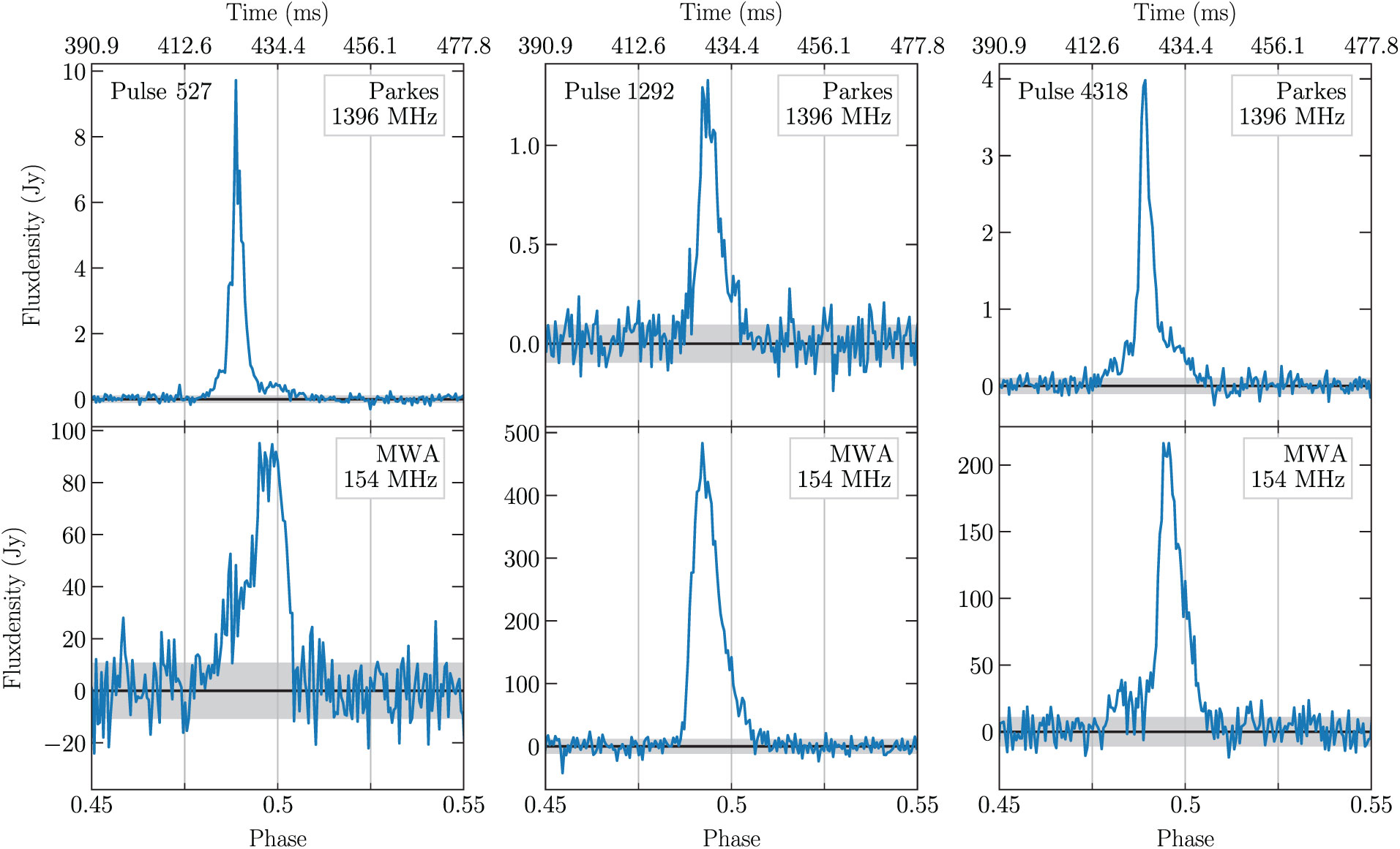
Figure 1. Examples of coincident single pulses from RRAT J2325−0530 at 1.4 GHz (Parkes; top row) and 154 MHz (MWA; bottom row). The pulses have been absolutely aligned, in which the same ephemeris was used to reduce the data sets. The number of rotations since the first simultaneously observed rotation of the pulsar is also given for each pair. Pulse 527 is the brightest pulse in the Parkes band of the coincident pulses, while pulse 1 292 is the brightest in the MWA band. Pulse 4318 is a relatively average example of a simultaneous pulse.
3.2. Profiles and polarisation
We combined the detected pulses into pseudo-integrated profiles which are shown in Figure 2. The profiles have been rotated by 0.5 turns for ease of comparison. No time alignment procedures have been applied to the profiles, and thus the profiles are absolutely aligned based on the ephemeris alone. The ‘knee’-like feature in the Parkes profile and the notch at the nominal profile peak are particularly interesting, given that the MWA profile is relativity smooth in comparison.c The residual dispersion smearing within the 10 kHz channels of the MWA data is (at worst) $\sim 0.5\,\text{ms}$
, which is similar in scale to the Parkes notch feature (
$\sim 0.5\,\text{ms}$
, which is similar in scale to the Parkes notch feature ( $\sim \!\!1\,\text{ms}$
); thus the smoothness of the MWA profile is possibly an artefact of incoherent dedispersion. The knee feature in the Parkes profile and the relatively extended rising edge of the MWA profile are also intriguing. These profile features would require coherently dedispersed, high S/N ratio profiles constructed from many hundreds or thousands of pulses, to examine in detail and to ensure their authenticity.
$\sim \!\!1\,\text{ms}$
); thus the smoothness of the MWA profile is possibly an artefact of incoherent dedispersion. The knee feature in the Parkes profile and the relatively extended rising edge of the MWA profile are also intriguing. These profile features would require coherently dedispersed, high S/N ratio profiles constructed from many hundreds or thousands of pulses, to examine in detail and to ensure their authenticity.
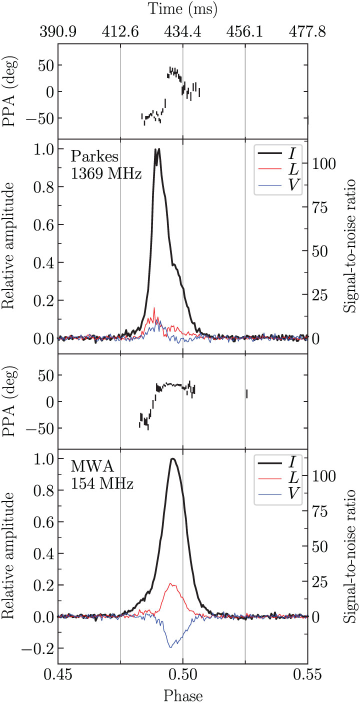
Figure 2. A pseudo-integrated profile, combining all single pulses with a $\rm S/N \geq 6$
. The profiles were produced using the same ephemeris and then rotated by 0.5 phase turns. Total intensity (Stokes I) is drawn in black, with linear (
$\rm S/N \geq 6$
. The profiles were produced using the same ephemeris and then rotated by 0.5 phase turns. Total intensity (Stokes I) is drawn in black, with linear ( $L=\sqrt{Q^2+U^2}$
) and circular (V) polarisation in red and blue, respectively. Above each profile is the linear polarisation position angle in degrees. Both profiles have been corrected for rotation measure (see Section 3.7).
$L=\sqrt{Q^2+U^2}$
) and circular (V) polarisation in red and blue, respectively. Above each profile is the linear polarisation position angle in degrees. Both profiles have been corrected for rotation measure (see Section 3.7).
The polarisation response of the MWA tied-array beam is currently undergoing self-consistency and cross-validation tests (e.g. Ord et al. Reference Ord, Tremblay, McSweeney, Bhat, Sobey, Mitchell, Hancock and Kirsten2019; Xue et al. Reference Xue, Ord, Tremblay, Bhat, Sobey, Meyers, McSweeney and Swainston2019). Nonetheless, we present here the first polarisation profile of RRAT J2325−0530 at 154 MHz and 1.4 GHz. The profiles have been corrected for Faraday rotation, removing the effects induced by the ISM and ionosphere (see Section 3.7). There is clearly substantial polarisation evolution with frequency in this case (see also Xue et al. Reference Xue, Ord, Tremblay, Bhat, Sobey, Meyers, McSweeney and Swainston2019). Even though the polarisation positional angle (PPA) has not been absolutely calibrated for the MWA, it is reassuring that the general shapes are similar. For both profiles, we were unable to fit the standard rotating vector model (RVM). In the case of the MWA profile, one possible reason for this is that scattering induced by the ISM can cause significant deviations from the normally expected RVM (S-like swing) shape (e.g. Karastergiou et al. Reference Karastergiou, Hotan, van Straten, McLaughlin and Ord2009).
3.3. Scintillation
After combining the single pulses as in Section 3.2, it was clear that RRAT J2325−0530 is affected by diffractive scintillation in the Parkes band. This was confirmed by examining the dynamic spectrum (see Figure 3). Due to the sporadic nature of RRAT emission, the diffractive scintillation pattern is sampled sparsely and irregularly in time. Consequently, performing the standard autocorrelation analysis (e.g. Gupta et al. Reference Gupta, Rickett and Lyne1994; Bhat et al. Reference Bhat, Rao and Gupta1999, Reference Bhat2018) is non-trivial. Furthermore, it is difficult to robustly constrain the scintillation parameters given that we only partially sample scintles in time or frequency at 1.4 GHz (which leads to large statistical uncertainties). At 154 MHz it is not immediately clear if there is any scintillation structure present, which suggests that the fine-channel width (10 kHz) is inadequate to capture the frequency structure. The results are summarised in Table 2. Given these complications, the diffractive scintillation parameters presented here should be considered with caution.
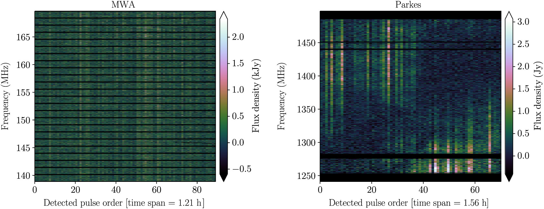
Figure 3. A dynamic spectrum of the brightest single pulses from RRAT J2325−0530 at 154 MHz (MWA; left) and 1.4 GHz (Parkes; right). The colour scale units are different for each dynamic spectrum (kJy for the MWA data, Jy for the Parkes data), and the x-axis represents the order in which the pulses were detected, with the total time spanned by these pulses given for context in the label. Note that this means the time axis is not continuous (i.e. each column of pixels, corresponding to a single pulse, is not necessarily contiguous with the previous column), unlike standard dynamic spectra. Nevertheless, it is clear that there is frequency and time structure indicative of diffractive scintillation in the Parkes data, though this is not the case for the MWA data. The black masked regions are those time and frequency samples excised by the RFI mitigation steps taken during post-processing of the single-pulse data, including coarse channel edges for the MWA, and the colour scale is linear.

Figure 4. The set of ACFs (grey) for the brightest pulses, and their best-fitting Gaussian model (black), from: (a) the MWA (15 pulses), and (b) Parkes (12 pulses). The MWA autocorrelations drop to zero by the first frequency lag bin and thus we are not able to even partially resolve the frequency structure. From the Parkes data we see structure, though the fact that the autocorrelations do not drop to zero before the last meaningful frequency lag bins indicates that we are not fully sampling a scintle, which is corroborated by the dynamic spectrum in Figure 3.
Table 2. Scintillation properties of RRAT J2325−0530.

3.3.1. Scintillation bandwidth
To estimate the scintillation bandwidth, we measured the mean flux density per frequency channel, $I(t,\nu)$
, for every pulse (i.e. the spectrum). Following Cordes et al. (Reference Cordes, Bhat, Hankins, McLaughlin and Kern2004), we then computed the intensity autocorrelation function (ACF),
$I(t,\nu)$
, for every pulse (i.e. the spectrum). Following Cordes et al. (Reference Cordes, Bhat, Hankins, McLaughlin and Kern2004), we then computed the intensity autocorrelation function (ACF),
 \begin{equation}
A(\delta\nu) = \langle I(t,\nu)\,I(t,\nu+\delta\nu)\rangle
\end{equation}
\begin{equation}
A(\delta\nu) = \langle I(t,\nu)\,I(t,\nu+\delta\nu)\rangle
\end{equation}
for each pulse, where $\delta\nu$
is the frequency lag representing a shift of one channel. For each
$\delta\nu$
is the frequency lag representing a shift of one channel. For each $A(\delta\nu)$
we fit a Gaussian to measure the standard deviation,
$A(\delta\nu)$
we fit a Gaussian to measure the standard deviation, $\sigma$
, and calculate the scintillation bandwidth as
$\sigma$
, and calculate the scintillation bandwidth as ${\nu_{\rm diss}}=\left(2\ln2\right)^{1/2}\sigma$
(which corresponds to the half-width at half-maximum of the Gaussian, e.g. Cordes Reference Cordes1986). The ACFs and models are normalised by the correlation value corresponding to zero frequency lag, which is calculated as the mean of the correlation value in the adjacent six frequency lag bins (three positive and three negative). In Figure 4, we show the ACFs and best-fit Gaussian models for the subset of pulses used to estimate the scintillation bandwidth.
${\nu_{\rm diss}}=\left(2\ln2\right)^{1/2}\sigma$
(which corresponds to the half-width at half-maximum of the Gaussian, e.g. Cordes Reference Cordes1986). The ACFs and models are normalised by the correlation value corresponding to zero frequency lag, which is calculated as the mean of the correlation value in the adjacent six frequency lag bins (three positive and three negative). In Figure 4, we show the ACFs and best-fit Gaussian models for the subset of pulses used to estimate the scintillation bandwidth.
Using the above method, we measure an average ${\nu_{\rm diss}}=102\pm 12\,\text{MHz}$
at
${\nu_{\rm diss}}=102\pm 12\,\text{MHz}$
at $1.4\,\text{GHz}$
(i.e. at Parkes) based on the subset of single pulses with
$1.4\,\text{GHz}$
(i.e. at Parkes) based on the subset of single pulses with ${\rm S/N}>40 (12/{70}\ \text{pulses})$
. This is nominally a lower limit given that over the observed bandwidth, we do not fully sample even one scintle. To calculate the expected characteristic scintillation bandwidth at MWA frequencies (154 MHz), we assume a frequency scaling index of
${\rm S/N}>40 (12/{70}\ \text{pulses})$
. This is nominally a lower limit given that over the observed bandwidth, we do not fully sample even one scintle. To calculate the expected characteristic scintillation bandwidth at MWA frequencies (154 MHz), we assume a frequency scaling index of $\gamma=-3.9\pm0.2$
(e.g. Bhat et al. Reference Bhat, Cordes, Camilo, Nice and Lorimer2004), where
$\gamma=-3.9\pm0.2$
(e.g. Bhat et al. Reference Bhat, Cordes, Camilo, Nice and Lorimer2004), where ${\nu_{\rm diss}}\propto\nu^{\gamma}$
. We find that the expected scintillation bandwidth is
${\nu_{\rm diss}}\propto\nu^{\gamma}$
. We find that the expected scintillation bandwidth is ${\nu_{\rm diss}}\approx 15\,\text{kHz}$
.
${\nu_{\rm diss}}\approx 15\,\text{kHz}$
.
Processing the single pulses with ${\rm S/N}>20 (15/{89}\ \text{pulses})$
from the MWA in the same way, we find that in all cases the ACF drops to zero by the first frequency lag bin, indicating that the scintillation bandwidth at 154 MHz is less than our channel width (i.e.
${\rm S/N}>20 (15/{89}\ \text{pulses})$
from the MWA in the same way, we find that in all cases the ACF drops to zero by the first frequency lag bin, indicating that the scintillation bandwidth at 154 MHz is less than our channel width (i.e. ${\nu _{{\rm{diss}}}} \mathbin{\lower.3ex\hbox{$\buildrel<\over
{\smash{\scriptstyle\sim}\vphantom{_x}}$}} 10{\mkern 1mu} {\rm{kHz}}$
). This indicates that the frequency scaling is steeper than
${\nu _{{\rm{diss}}}} \mathbin{\lower.3ex\hbox{$\buildrel<\over
{\smash{\scriptstyle\sim}\vphantom{_x}}$}} 10{\mkern 1mu} {\rm{kHz}}$
). This indicates that the frequency scaling is steeper than $\gamma=-3.9$
. If we take the nominal measured values of
$\gamma=-3.9$
. If we take the nominal measured values of ${\nu_{\rm diss}}$
at each frequency, and again use the previous defined scaling relation, we find that
${\nu_{\rm diss}}$
at each frequency, and again use the previous defined scaling relation, we find that $\gamma \approx -4.2$
, which is steeper than the empirically derived global scaling index (Bhat et al. Reference Bhat, Cordes, Camilo, Nice and Lorimer2004). We note that nearby pulsars tend to show a steeper scaling index, approaching the extremum (Kolmogorov turbulence) scaling of
$\gamma \approx -4.2$
, which is steeper than the empirically derived global scaling index (Bhat et al. Reference Bhat, Cordes, Camilo, Nice and Lorimer2004). We note that nearby pulsars tend to show a steeper scaling index, approaching the extremum (Kolmogorov turbulence) scaling of $\gamma=-4.4$
, due to the decreased probability of intervening structures in the ISM that would serve to shallow the scaling index.
$\gamma=-4.4$
, due to the decreased probability of intervening structures in the ISM that would serve to shallow the scaling index.
Finally, the scintillation characteristics are statistical quantities; thus the sample variance must be included in all quantities derived from the scintillation properties, especially when a small number of scintles is observed. This uncertainty is given by $\sigma_{\rm stat} \approx N_{\rm scint}^{-1/2}$
, where the number of scintles observed,
$\sigma_{\rm stat} \approx N_{\rm scint}^{-1/2}$
, where the number of scintles observed, $N_{\rm scint}$
, in the total observing time,
$N_{\rm scint}$
, in the total observing time, $t_{\rm obs}$
, over a bandwidth,
$t_{\rm obs}$
, over a bandwidth, $B_{\rm obs}$
, is given by
$B_{\rm obs}$
, is given by
 \begin{equation}
N_{\rm scint} = \left(\frac{B_{\rm obs}t_{\rm obs}}{{\nu_{\rm diss}} {\tau_{\rm diss}}}\right)f_d,
\end{equation}
\begin{equation}
N_{\rm scint} = \left(\frac{B_{\rm obs}t_{\rm obs}}{{\nu_{\rm diss}} {\tau_{\rm diss}}}\right)f_d,
\end{equation}
where $f_d$
is a filling fraction that describes how much of the observed frequency-time phase space contains signal (e.g. Bhat et al. Reference Bhat, Rao and Gupta1999), which we assume to be
$f_d$
is a filling fraction that describes how much of the observed frequency-time phase space contains signal (e.g. Bhat et al. Reference Bhat, Rao and Gupta1999), which we assume to be $f_d \approx 0.5$
based on the Parkes dynamic spectrum in Figure 3. For the MWA, where the scintles are on the order of 10 kHz wide, this factor is negligible (
$f_d \approx 0.5$
based on the Parkes dynamic spectrum in Figure 3. For the MWA, where the scintles are on the order of 10 kHz wide, this factor is negligible ( $N_{\rm scint}\approx 2\times 10^5$
and
$N_{\rm scint}\approx 2\times 10^5$
and $\sigma_{\rm stat} \sim\! 0.2\%$
, or
$\sigma_{\rm stat} \sim\! 0.2\%$
, or $20\,\text{Hz}$
). However, in the case of Parkes, we clearly sample far fewer scintles (
$20\,\text{Hz}$
). However, in the case of Parkes, we clearly sample far fewer scintles ( $N_{\rm scint}\approx 2$
); ergo, the sampling error is
$N_{\rm scint}\approx 2$
); ergo, the sampling error is $\sigma_{\rm stat} \approx 70\%$
and
$\sigma_{\rm stat} \approx 70\%$
and ${\nu_{\rm diss}} = {102\pm 72}\,\text{MHz}$
(where the final error is the quadrature sum of the fitting error and statistical error).
${\nu_{\rm diss}} = {102\pm 72}\,\text{MHz}$
(where the final error is the quadrature sum of the fitting error and statistical error).
3.3.2. Scintillation time scale
The RRAT emission irregularly samples the scintillation pattern which makes estimating the scintillation time scale, ${\tau_{\rm diss}}$
, difficult. Nevertheless, we calculate the intensity cross-correlation,
${\tau_{\rm diss}}$
, difficult. Nevertheless, we calculate the intensity cross-correlation,
 \begin{equation}
\rho(\tau, \delta\nu=0)=\langle \Delta I(t, \nu) \Delta I(t+\tau, \nu+\delta\nu)\rangle
\end{equation}
\begin{equation}
\rho(\tau, \delta\nu=0)=\langle \Delta I(t, \nu) \Delta I(t+\tau, \nu+\delta\nu)\rangle
\end{equation}
between every mean-subtracted single-pulse spectra, $\Delta I(t,\nu)$
, and subsequent pulses, while recording the corresponding time lag,
$\Delta I(t,\nu)$
, and subsequent pulses, while recording the corresponding time lag, $\tau$
, as the number of pulsar rotations between the correlated pulse spectra.d We average the correlation coefficients for each time lag and then re-bin the results such that there is one
$\tau$
, as the number of pulsar rotations between the correlated pulse spectra.d We average the correlation coefficients for each time lag and then re-bin the results such that there is one $\rho(\tau,0)$
per
$\rho(\tau,0)$
per $150\,\text{s}$
for the Parkes data. In Figure 5, we plot these correlation coefficients against time lag.
$150\,\text{s}$
for the Parkes data. In Figure 5, we plot these correlation coefficients against time lag.
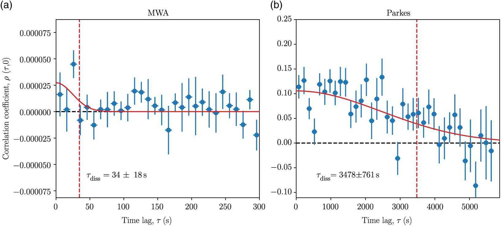
Figure 5. Mean correlation coefficients of individual pulse spectra, binned into: (a) 10-s intervals for MWA data, and (b) 150-s intervals for Parkes data. The Gaussian fit to the data (red, solid line) is weighted based on the standard error of each of the points, where the $1/e$
-half-width of the Gaussian corresponds to the scintillation time scale. We measure a scintillation time scale
$1/e$
-half-width of the Gaussian corresponds to the scintillation time scale. We measure a scintillation time scale ${\tau_{\rm diss}}={3478\pm 2550}\,\text{s}$
at
${\tau_{\rm diss}}={3478\pm 2550}\,\text{s}$
at $1.4\,\text{GHz}$
, and
$1.4\,\text{GHz}$
, and ${\tau_{\rm diss}}={34\pm 18}\,\text{s}$
at
${\tau_{\rm diss}}={34\pm 18}\,\text{s}$
at $154\,\text{MHz}$
, marked by the vertical dashed red lines.
$154\,\text{MHz}$
, marked by the vertical dashed red lines.
The scintillation time scale is the $1/e$
-half-width of the fitted Gaussian (
$1/e$
-half-width of the fitted Gaussian ( ${\tau_{\rm diss}}=\sqrt{2}\sigma$
), where the mean is forced to zero, which we measure to be
${\tau_{\rm diss}}=\sqrt{2}\sigma$
), where the mean is forced to zero, which we measure to be ${\tau_{\rm diss}} = 3478\pm 761\,\text{s}$
at
${\tau_{\rm diss}} = 3478\pm 761\,\text{s}$
at $1.4\,\text{GHz}$
. Including the relative sampling error of
$1.4\,\text{GHz}$
. Including the relative sampling error of $\sim 70\%$
, we find that
$\sim 70\%$
, we find that ${\tau_{\rm diss}} = {3478\pm 2550}\,\text{s}$
. Additionally, we can estimate the expected refractive interstellar scintillation (RISS) time scale (e.g. Rickett Reference Rickett1990) at 1.4 GHz, where
${\tau_{\rm diss}} = {3478\pm 2550}\,\text{s}$
. Additionally, we can estimate the expected refractive interstellar scintillation (RISS) time scale (e.g. Rickett Reference Rickett1990) at 1.4 GHz, where $\tau_{\rm riss} = {\tau_{\rm diss}}\left(\nu/{\nu_{\rm diss}}\right) \approx 13\,\text{h}$
. These values should be considered with caution given that, as for the scintillation bandwidth, we do not actually sample a full scintle over the 1.5 h observation.
$\tau_{\rm riss} = {\tau_{\rm diss}}\left(\nu/{\nu_{\rm diss}}\right) \approx 13\,\text{h}$
. These values should be considered with caution given that, as for the scintillation bandwidth, we do not actually sample a full scintle over the 1.5 h observation.
Scaling the decorrelation time from $1.4\,\text{GHz}$
, assuming
$1.4\,\text{GHz}$
, assuming ${\tau_{\rm diss}}\propto \nu^{1.2}$
, implies
${\tau_{\rm diss}}\propto \nu^{1.2}$
, implies ${\tau_{\rm diss}}\approx 250\pm 185\,\text{s}$
at
${\tau_{\rm diss}}\approx 250\pm 185\,\text{s}$
at $154\,\text{MHz}$
. Using the same technique as above on the MWA data, except re-binning to one
$154\,\text{MHz}$
. Using the same technique as above on the MWA data, except re-binning to one $\rho(\tau,0)$
per
$\rho(\tau,0)$
per $10\,\text{s}$
(given the expected
$10\,\text{s}$
(given the expected ${\tau_{\rm diss}}$
), we find that we are severely limited by the S/N ratio of our detected pulses. This is due to the scintillation bandwidth being on the order of, or less than, the channel width. The estimated scintillation time scale is a factor of 7 less than expected, where
${\tau_{\rm diss}}$
), we find that we are severely limited by the S/N ratio of our detected pulses. This is due to the scintillation bandwidth being on the order of, or less than, the channel width. The estimated scintillation time scale is a factor of 7 less than expected, where ${\tau_{\rm diss}} = 34\pm 18\,\text{s}$
. Visually inspecting Figure 5, one can see that the correlation coefficients, even after averaging in time, are consistent with noise except for one outlier. Furthermore, the quality of the Gaussian fit changes drastically depending on how the correlation coefficients are averaged, and generally results in an unconstrained estimate of
${\tau_{\rm diss}} = 34\pm 18\,\text{s}$
. Visually inspecting Figure 5, one can see that the correlation coefficients, even after averaging in time, are consistent with noise except for one outlier. Furthermore, the quality of the Gaussian fit changes drastically depending on how the correlation coefficients are averaged, and generally results in an unconstrained estimate of ${\tau_{\rm diss}}$
(i.e. undefined uncertainty or failing to find an adequate fit altogether). For these reasons we caution against interpretation of the measured scintillation parameters at 154 MHz alone.
${\tau_{\rm diss}}$
(i.e. undefined uncertainty or failing to find an adequate fit altogether). For these reasons we caution against interpretation of the measured scintillation parameters at 154 MHz alone.
3.3.3. Scintillation velocity and turbulence strength
We can calculate the scintillation velocity—as a proxy to the RRAT space velocity—under the caveats that: both ${\nu_{\rm diss}}$
and
${\nu_{\rm diss}}$
and ${\tau_{\rm diss}}$
are nominally lower limits; we do not know the relative distance of the scattering screen to the pulsar; and there is a factor of two discrepancy in distance estimates, where
${\tau_{\rm diss}}$
are nominally lower limits; we do not know the relative distance of the scattering screen to the pulsar; and there is a factor of two discrepancy in distance estimates, where $D=0.7$
and
$D=0.7$
and $1.49\,\text{kpc}$
, from NE2001 (Cordes & Lazio Reference Cordes and Lazio2002, Reference Cordes and Lazio2003) and YMW2016 (Yao et al. Reference Yao, Manchester and Wang2017) models, respectively. We assign a 25% uncertainty to each distance estimate. The scintillation velocity is given by
$1.49\,\text{kpc}$
, from NE2001 (Cordes & Lazio Reference Cordes and Lazio2002, Reference Cordes and Lazio2003) and YMW2016 (Yao et al. Reference Yao, Manchester and Wang2017) models, respectively. We assign a 25% uncertainty to each distance estimate. The scintillation velocity is given by
 \begin{equation}
V_{\rm iss} = A_{\rm iss} \frac{\left(Dx{\nu_{\rm diss}}\right)^{1/2}}{\nu{\tau_{\rm diss}}},
\end{equation}
\begin{equation}
V_{\rm iss} = A_{\rm iss} \frac{\left(Dx{\nu_{\rm diss}}\right)^{1/2}}{\nu{\tau_{\rm diss}}},
\end{equation}
where $D = D_{\rm os} + D_{\rm ps}$
is the total distance to the pulsar in kpc;
$D = D_{\rm os} + D_{\rm ps}$
is the total distance to the pulsar in kpc; $D_{\rm os}$
and
$D_{\rm os}$
and $D_{\rm ps}$
are the distances from the screen to the observer and pulsar respectively in kpc;
$D_{\rm ps}$
are the distances from the screen to the observer and pulsar respectively in kpc; $x = D_{\rm os} / D_{\rm ps}$
(in this case we assume
$x = D_{\rm os} / D_{\rm ps}$
(in this case we assume $x=1$
, i.e. the screen is located exactly half way between the observer and the pulsar);
$x=1$
, i.e. the screen is located exactly half way between the observer and the pulsar); $\nu$
is the observing frequency in GHz;
$\nu$
is the observing frequency in GHz; ${\nu_{\rm diss}}$
is in MHz, and
${\nu_{\rm diss}}$
is in MHz, and ${\tau_{\rm diss}}$
in seconds. The scaling constant
${\tau_{\rm diss}}$
in seconds. The scaling constant $A_{\rm iss}=2.53\times 10^4\,{\rm km\,s^{-1}}$
is derived for a homogeneously distributed ISM with a Kolmogorov turbulence spectrum (Cordes & Rickett Reference Cordes and Rickett1998), which appears to be a valid approximation for this pulsar given the scintillation frequency scaling index calculated in Section 3.3.1. For a distance
$A_{\rm iss}=2.53\times 10^4\,{\rm km\,s^{-1}}$
is derived for a homogeneously distributed ISM with a Kolmogorov turbulence spectrum (Cordes & Rickett Reference Cordes and Rickett1998), which appears to be a valid approximation for this pulsar given the scintillation frequency scaling index calculated in Section 3.3.1. For a distance $D=0.70\pm0.18\,\text{kpc}$
we find
$D=0.70\pm0.18\,\text{kpc}$
we find $V_{\rm iss}={44\pm 36}\,{\rm km\,s^{-1}}$
, while for
$V_{\rm iss}={44\pm 36}\,{\rm km\,s^{-1}}$
, while for $D=1.49\pm0.37\,\text{kpc}$
,
$D=1.49\pm0.37\,\text{kpc}$
, $V_{\rm iss}={64\pm 52}\,{\rm km\,s^{-1}}$
. The uncertainties correspond to the quadrature sum of the scintillation bandwidth, scintillation time scale, and distance errors, given by
$V_{\rm iss}={64\pm 52}\,{\rm km\,s^{-1}}$
. The uncertainties correspond to the quadrature sum of the scintillation bandwidth, scintillation time scale, and distance errors, given by
 \begin{align}
\Delta V_{\rm iss} &= \left(
\left[\frac{\partial V_{\rm iss}}{\partial {\nu_{\rm diss}}}\Delta{\nu_{\rm diss}}\right]^2 \right. + \nonumber\\
&\qquad\left[\frac{\partial V_{\rm iss}}{\partial {\tau_{\rm diss}}}\Delta{\tau_{\rm diss}}\right]^2 +
\left. \left[\frac{\partial V_{\rm iss}}{\partial D}\Delta D\right]^2 \right)^{1/2},
\end{align}
\begin{align}
\Delta V_{\rm iss} &= \left(
\left[\frac{\partial V_{\rm iss}}{\partial {\nu_{\rm diss}}}\Delta{\nu_{\rm diss}}\right]^2 \right. + \nonumber\\
&\qquad\left[\frac{\partial V_{\rm iss}}{\partial {\tau_{\rm diss}}}\Delta{\tau_{\rm diss}}\right]^2 +
\left. \left[\frac{\partial V_{\rm iss}}{\partial D}\Delta D\right]^2 \right)^{1/2},
\end{align}
where $\Delta X$
represents the uncertainty in parameter X. We did not calculate the scintillation velocities from the MWA data since we do not have reliable estimates of
$\Delta X$
represents the uncertainty in parameter X. We did not calculate the scintillation velocities from the MWA data since we do not have reliable estimates of ${\nu_{\rm diss}}$
and
${\nu_{\rm diss}}$
and ${\tau_{\rm diss}}$
(see Table 2).
${\tau_{\rm diss}}$
(see Table 2).
We can also place limits on the mean turbulence strength, ${\overline{C^2_{\rm n}}}$
, along the line-of-sight. Assuming Kolmogorov turbulence, the mean turbulence strength in units of
${\overline{C^2_{\rm n}}}$
, along the line-of-sight. Assuming Kolmogorov turbulence, the mean turbulence strength in units of ${\rm m^{-20/3}}$
is
${\rm m^{-20/3}}$
is
 \begin{equation}
{\overline{C^2_{\rm n}}} \approx 0.002\,\nu^{11/3} D^{-11/6} {\nu_{\rm diss}^{-5/6}},
\end{equation}
\begin{equation}
{\overline{C^2_{\rm n}}} \approx 0.002\,\nu^{11/3} D^{-11/6} {\nu_{\rm diss}^{-5/6}},
\end{equation}
(cf. Eq. 9 of Cordes et al. Reference Cordes, Wolszczan, Dewey, Blaskiewicz and Stinebring1990) where $\nu$
, D, and
$\nu$
, D, and ${\nu_{\rm diss}}$
are in the same units as for Eq. (4). Given the range in distances, we find that the corresponding range in turbulence strength is
${\nu_{\rm diss}}$
are in the same units as for Eq. (4). Given the range in distances, we find that the corresponding range in turbulence strength is ${\overline{C^2_{\rm n}}}\approx (7\text{-}28)\times 10^{-5}\,{\rm m^{-20/3}}$
at 1.4 GHz, and note that given the lower limit on
${\overline{C^2_{\rm n}}}\approx (7\text{-}28)\times 10^{-5}\,{\rm m^{-20/3}}$
at 1.4 GHz, and note that given the lower limit on ${\nu_{\rm diss}}$
from Parkes data we can only confidently say that
${\nu_{\rm diss}}$
from Parkes data we can only confidently say that $\overline {C_{\rm{n}}^2} \mathbin{\lower.3ex\hbox{$\buildrel<\over
{\smash{\scriptstyle\sim}\vphantom{_x}}$}} 2.8 \times {10^{ - 4}}{\mkern 1mu} {{\rm{m}}^{{\rm{ - 20/3}}}}$
.
$\overline {C_{\rm{n}}^2} \mathbin{\lower.3ex\hbox{$\buildrel<\over
{\smash{\scriptstyle\sim}\vphantom{_x}}$}} 2.8 \times {10^{ - 4}}{\mkern 1mu} {{\rm{m}}^{{\rm{ - 20/3}}}}$
.
3.4. Spectral index
A cross-matched list of single pulses was created from the independent MWA and Parkes pulse data sets using the stilts table manipulation software (Taylor Reference Taylor, Gabriel, Arviset, Ponz and Enrique2006). After the cross-matching stage, there were 45 pulses coincident in both bands. For each of these pulses we used their measured fluences to calculate a spectral index, the distribution of which is shown in Figure 6 along with an indicator of the normal pulsar population spectral index range in grey.

Figure 6. Spectral index distribution for detected simultaneous pulses between the MWA and Parkes. The red solid line is a Gaussian fit to the distribution, and the pink envelope represents the $1-\sigma$
confidence interval of the model. Error bars on the points are Poisson uncertainties only. The mean spectral index is
$1-\sigma$
confidence interval of the model. Error bars on the points are Poisson uncertainties only. The mean spectral index is $\alpha=-2.2\pm 0.1$
with a standard deviation of
$\alpha=-2.2\pm 0.1$
with a standard deviation of $\sigma=0.4\pm 0.1$
. The grey-shaded region is the typical distribution of spectral indices, with a mean of
$\sigma=0.4\pm 0.1$
. The grey-shaded region is the typical distribution of spectral indices, with a mean of $\langle\alpha\rangle=-1.6$
and standard deviation of
$\langle\alpha\rangle=-1.6$
and standard deviation of $\sigma=0.5$
(Jankowski et al. Reference Jankowski, van Straten, Keane, Bailes, Barr, Johnston and Kerr2018).
$\sigma=0.5$
(Jankowski et al. Reference Jankowski, van Straten, Keane, Bailes, Barr, Johnston and Kerr2018).
We measure a mean single-pulse spectral index of $\alpha_{154}^{1369}=-2.2\pm 0.1$
which is relatively steep compared to mean spectral index observed in the typical pulsar population, where
$\alpha_{154}^{1369}=-2.2\pm 0.1$
which is relatively steep compared to mean spectral index observed in the typical pulsar population, where $\langle\alpha\rangle\approx -1.6$
(see e.g. Maron et al. Reference Maron, Kijak, Kramer and Wielebinski2000; Bates et al. Reference Bates, Lorimer and Verbiest2013; Jankowski et al. Reference Jankowski, van Straten, Keane, Bailes, Barr, Johnston and Kerr2018). The range of single-pulse spectral indices we measure is
$\langle\alpha\rangle\approx -1.6$
(see e.g. Maron et al. Reference Maron, Kijak, Kramer and Wielebinski2000; Bates et al. Reference Bates, Lorimer and Verbiest2013; Jankowski et al. Reference Jankowski, van Straten, Keane, Bailes, Barr, Johnston and Kerr2018). The range of single-pulse spectral indices we measure is $-2.8 < \alpha_{154}^{1369} < -1.5$
. The steep spectral index we measure seems to agree empirically with the detections reported in the literature, given that RRAT J2325−0530 has been detected multiple times with low-frequency observations in the past from the GBT (350 MHz), LOFAR (150 MHz), and LWA1 (30–80 MHz).
$-2.8 < \alpha_{154}^{1369} < -1.5$
. The steep spectral index we measure seems to agree empirically with the detections reported in the literature, given that RRAT J2325−0530 has been detected multiple times with low-frequency observations in the past from the GBT (350 MHz), LOFAR (150 MHz), and LWA1 (30–80 MHz).
3.5. Fluence distributions
From the detected pulses, we constructed fluence (pulse energy) distributions for each band. To these distributions, we fit three relativity common models using the Python lmfit modulee: a power law (PL), a truncated exponential (TE; functionally the same as Eq. 3 of Mickaliger et al. Reference Mickaliger, McEwen, McLaughlin and Lorimer2018), and a log-normal (LN) distribution. The relevant functional forms are:
 \begin{align}
N_{\rm PL}(x) &= Ax^{-\beta},\end{align}
\begin{align}
N_{\rm PL}(x) &= Ax^{-\beta},\end{align}
 \begin{align}
N_{\rm TE}(x) &= Bx^{-\zeta}e^{-\lambda x},\end{align}
\begin{align}
N_{\rm TE}(x) &= Bx^{-\zeta}e^{-\lambda x},\end{align}
 \begin{align}
N_{\rm LN}(x) &= \frac{C}{x\sigma}\exp\left[-\frac{(\ln x -\mu)^2}{2\sigma^2}\right],
\end{align}
\begin{align}
N_{\rm LN}(x) &= \frac{C}{x\sigma}\exp\left[-\frac{(\ln x -\mu)^2}{2\sigma^2}\right],
\end{align}
where $N(x)\,{\rm d}x$
is the number of pulses at fluence x, A, B, and C are arbitrary scaling constants,
$N(x)\,{\rm d}x$
is the number of pulses at fluence x, A, B, and C are arbitrary scaling constants, $\beta$
and
$\beta$
and $\zeta$
are PL exponents,
$\zeta$
are PL exponents, $\lambda$
is a decay parameter, and
$\lambda$
is a decay parameter, and $\mu$
and
$\mu$
and $\sigma$
are the location and scale parameters for the normally distributed logarithm (i.e.
$\sigma$
are the location and scale parameters for the normally distributed logarithm (i.e. $\ln x$
). Note that in this case the PLs are fitted only to the pulses which have fluences greater than 0.8 and 0.006 Jy s for the MWA and Parkes, respectively. These cut-offs were chosen to coincide roughly with where the distributions peak. Without these restrictions, the PL model is a poor fit to the data. The data and fitted models are shown in Figure 7, and model parameters (with standard errors) are given in Table 3. In general it appears that a LN distribution is favoured, though see Section 4.3 for further discussion.
$\ln x$
). Note that in this case the PLs are fitted only to the pulses which have fluences greater than 0.8 and 0.006 Jy s for the MWA and Parkes, respectively. These cut-offs were chosen to coincide roughly with where the distributions peak. Without these restrictions, the PL model is a poor fit to the data. The data and fitted models are shown in Figure 7, and model parameters (with standard errors) are given in Table 3. In general it appears that a LN distribution is favoured, though see Section 4.3 for further discussion.

Figure 7. Pulse fluence (energy) distributions for single pulses detected with the MWA (left) and Parkes (right). We fitted a power law (blue), truncated exponential (orange), and log-normal (green) distribution model to the binned single-pulse fluences. The error bars represent statistical (Poisson) errors only. The reduced chi-squared values of the fits are given in the legend. The power law cut-off for each frequency is indicated by the blue vertical dotted lines.
Table 3. Best-fit parameters for trial fluence distribution models.

* Restricted to fitting pulses with fluences greater than 0.8 and 0.06 Jy s for the MWA and Parkes (see text).
a The location ( $\mu$
) and scale (
$\mu$
) and scale ( $\sigma$
) parameters, as defined by Python’s scipy.stats.lognorm.
$\sigma$
) parameters, as defined by Python’s scipy.stats.lognorm.
3.6. Pulse rates and clustering
We measured a total of 89 and 70 pulses with $\rm{S/N}\geq 6$
with the MWA and Parkes, respectively. These detections correspond to pulse rates of
$\rm{S/N}\geq 6$
with the MWA and Parkes, respectively. These detections correspond to pulse rates of $73\pm 7\,{\rm h^{-1}}$
above a peak flux density of 65 Jy at 154 MHz, and
$73\pm 7\,{\rm h^{-1}}$
above a peak flux density of 65 Jy at 154 MHz, and $43\pm 5\,{\rm h^{-1}}$
above a peak flux density of 0.6 Jy at 1.4 GHz, where the uncertainties correspond to the Poisson counting error. The pulse rates we measure, as well as those in the literature, are presented in Table 4. In the case of the minimum detectable flux density for the LOFAR results (Karako-Argaman et al. Reference Karako-Argaman2015), we assign a gain for the core stations of
$43\pm 5\,{\rm h^{-1}}$
above a peak flux density of 0.6 Jy at 1.4 GHz, where the uncertainties correspond to the Poisson counting error. The pulse rates we measure, as well as those in the literature, are presented in Table 4. In the case of the minimum detectable flux density for the LOFAR results (Karako-Argaman et al. Reference Karako-Argaman2015), we assign a gain for the core stations of $0.68\mathrm{\,K\,Jy^{-1}}$
(based on estimates of the collecting area of van Haarlem et al. (Reference van Haarlem2013), modified by a projection factor of
$0.68\mathrm{\,K\,Jy^{-1}}$
(based on estimates of the collecting area of van Haarlem et al. (Reference van Haarlem2013), modified by a projection factor of $\cos^2(\pi/6)=3/4$
assuming a best-case scenario where the source was observed at
$\cos^2(\pi/6)=3/4$
assuming a best-case scenario where the source was observed at $\sim 60\,\text{deg}$
elevation) and add 250 K to the nominal 400 K receiver temperature in an attempt to include sky noise contributions. Using these values, we estimate a minimum detectable flux density of
$\sim 60\,\text{deg}$
elevation) and add 250 K to the nominal 400 K receiver temperature in an attempt to include sky noise contributions. Using these values, we estimate a minimum detectable flux density of $\sim 21\,\text{Jy}$
, assuming the same caveats of the original estimate (i.e.
$\sim 21\,\text{Jy}$
, assuming the same caveats of the original estimate (i.e. $\text{SNR}\geq 5 $
and 10 ms pulse width).
$\text{SNR}\geq 5 $
and 10 ms pulse width).
Table 4. Pulse rates and nominal detection sensitivity for single pulses from RRAT J2325−0530.

References — T + 16: Taylor et al. (Reference Taylor, Stovall, McCrackan, McLaughlin, Miller, Karako-Argaman, Dowell and Schinzel2016), KA + 15: Karako-Argaman et al. (Reference Karako-Argaman2015).
a Fluence limits from other works were estimated by calculating the area under a tophat with amplitude equal to the corresponding sensitivity and a width of 5 ms (mean effective width of pulses measured in this work).
b Over the full observed bandwidth, which was at best 60 MHz. Individual sub-band sensitivities are therefore $\sim\!120$
Jy.
$\sim\!120$
Jy.
c Split into 2–3 h blocks over 10 days spread throughout late-2013 and late-2014, see Taylor et al. (Reference Taylor, Stovall, McCrackan, McLaughlin, Miller, Karako-Argaman, Dowell and Schinzel2016) for details.
d Calculated using eq. 1 and observing parameters from Table 1 (though see text regarding LOFAR parameters) of Karako-Argaman et al. (Reference Karako-Argaman2015), assuming a detection threshold of ${\rm S/N}\geq 5$
.
${\rm S/N}\geq 5$
.
We also examine the distribution of the number of rotations between subsequent pulses (‘wait times’) within our observation. These wait times are presented in Figure 8. In this case, we binned the wait times into 50 equally spaced intervals, ranging from one pulsar rotation to the maximum wait time, which corresponds to 596 rotations ( $\sim\!517\,\text{s}$
) in the Parkes data. The median wait times for the MWA and Parkes pulses are 52 and 68 rotations, respectively. In both the MWA and Parkes data, the minimum wait time is one rotation. The maximum wait time in the MWA data is 184 rotations (i.e.
$\sim\!517\,\text{s}$
) in the Parkes data. The median wait times for the MWA and Parkes pulses are 52 and 68 rotations, respectively. In both the MWA and Parkes data, the minimum wait time is one rotation. The maximum wait time in the MWA data is 184 rotations (i.e. $\sim\!159\,\text{s}$
), with 75 instances of wait times less than 100 rotations. For Parkes, the maximum wait time is substantially longer, at 596 rotations (i.e.
$\sim\!159\,\text{s}$
), with 75 instances of wait times less than 100 rotations. For Parkes, the maximum wait time is substantially longer, at 596 rotations (i.e. $\sim\!520\,\text{s}$
), and there are 46 wait times less than 100 rotations. Given the different sensitivity thresholds of each telescope, it is difficult to quantitatively compare these numbers, especially since scaling thresholds and selecting pulses from either sample only adds to the issue of small number statistics in this case.
$\sim\!520\,\text{s}$
), and there are 46 wait times less than 100 rotations. Given the different sensitivity thresholds of each telescope, it is difficult to quantitatively compare these numbers, especially since scaling thresholds and selecting pulses from either sample only adds to the issue of small number statistics in this case.

Figure 8. Histogram of the number of rotations between subsequent pulses (i.e. wait times) for the MWA pulses (top) and Parkes pulses (bottom). The blue solid lines are a fit to an exponential distribution, and the light blue-shaded regions represent the 99% confidence interval based on the fitting uncertainties. Wait times were binned into 50 equally spaced bins ranging from 1 rotation to 596 rotations (i.e. 517 s, the maximum wait time in either frequency band). The reduced chi-square statistic, $\chi_r^2$
, for each fit is 2.15 and 1.24 for the MWA and Parkes, respectively.
$\chi_r^2$
, for each fit is 2.15 and 1.24 for the MWA and Parkes, respectively.
If the single-pulse emission is produced by a Poisson (random) process, then we would expect that the time between events (i.e. the wait times) would be exponentially distributed ( $N(x)\,{\rm d}x \propto e^{-\eta x}$
). After fitting each sample independently, we find that the exponents are similar, where
$N(x)\,{\rm d}x \propto e^{-\eta x}$
). After fitting each sample independently, we find that the exponents are similar, where $\eta_{\rm MWA} = 0.013\pm 0.001$
for the MWA, and
$\eta_{\rm MWA} = 0.013\pm 0.001$
for the MWA, and $\eta_{\rm PKS} = 0.009\,\pm\,0.001$
for the Parkes data. From these data, it is unclear whether there is a significant excess beyond what would be expected of pulse events drawn from a Poisson distributed process (an exponential distribution has been fitted to the wait times, see Figure 8). In the context of the general pulsar population, similar work has to be done for nulling pulsars, noting examples of clustering (e.g. Redman & Rankin Reference Redman and Rankin2009), and of random processes (e.g. Gajjar et al. Reference Gajjar and Kramer2012). The latter is reasonably consistent with what we find for RRAT J2325−0530. Ultimately, we are limited in this case by the number of single-pulse detections, and note that the Parkes wait time distribution will be biased by the scintillation effects.
$\eta_{\rm PKS} = 0.009\,\pm\,0.001$
for the Parkes data. From these data, it is unclear whether there is a significant excess beyond what would be expected of pulse events drawn from a Poisson distributed process (an exponential distribution has been fitted to the wait times, see Figure 8). In the context of the general pulsar population, similar work has to be done for nulling pulsars, noting examples of clustering (e.g. Redman & Rankin Reference Redman and Rankin2009), and of random processes (e.g. Gajjar et al. Reference Gajjar and Kramer2012). The latter is reasonably consistent with what we find for RRAT J2325−0530. Ultimately, we are limited in this case by the number of single-pulse detections, and note that the Parkes wait time distribution will be biased by the scintillation effects.
3.7. Rotation measure
The rotation measure (RM) quantifies the degree of Faraday rotation that the radio emission from a source experiences after traversing the ISM, and was traditionally measured by calculating the change in linear polarisation angle across the observing band (e.g. Noutsos et al. Reference Noutsos, Johnston, Kramer and Karastergiou2008; Han et al. Reference Han, Manchester, van Straten and Demorest2018). We used the psrchive RM fitting routine, rmfit, which effectively implements the RM synthesis method (e.g. Brentjens & de Bruyn Reference Brentjens and de Bruyn2005), to determine the nominal RM of the Parkes and MWA data based on the polarisation properties of the pseudo-integrated pulse profiles (Figure 2).
The ionosphere can significantly contribute to the measured RM; thus we calculated the ionospheric contribution for both Parkes and the MWA using ionFRf (Sotomayor-Beltran et al. Reference Sotomayor-Beltran2013), using the latest version of the International Geomagnetic Reference Field (IGRF12; Thébault et al. Reference Thébault2015) and the International Global Navigation Satellite System Service vertical total electron content maps (e.g. Hernández-Pajares et al. Reference Hernández-Pajares2009). The RM contribution from the ISM is given by $\rm RM_{ISM} = RM_{obs} - RM_{ion}$
, the values for which are given in Table 5. The ionosphere was relatively quiet during the observations, but is still the dominant source of uncertainty in estimating the RM imparted by the ISM for the MWA measurements.
$\rm RM_{ISM} = RM_{obs} - RM_{ion}$
, the values for which are given in Table 5. The ionosphere was relatively quiet during the observations, but is still the dominant source of uncertainty in estimating the RM imparted by the ISM for the MWA measurements.
Table 5. Rotation measure estimate for RRAT J2325−0530.

After ionospheric correction, the ISM contribution to the RM along this line-of-sight based on the MWA data is $\rm RM_{ISM}=3.85\pm 0.12\,rad\,m^{-2}$
. While the Parkes data measurement is less constraining, it does agree within uncertainty. Given the RM and DM, we can estimate the average line-of-sight magnetic field strength using the approximation
$\rm RM_{ISM}=3.85\pm 0.12\,rad\,m^{-2}$
. While the Parkes data measurement is less constraining, it does agree within uncertainty. Given the RM and DM, we can estimate the average line-of-sight magnetic field strength using the approximation
 \begin{equation}
\langle B_\parallel\rangle \approx 1.23\left(\frac{\rm RM}{\rm DM}\right) \mathrm{\,\mu G},
\end{equation}
\begin{equation}
\langle B_\parallel\rangle \approx 1.23\left(\frac{\rm RM}{\rm DM}\right) \mathrm{\,\mu G},
\end{equation}
where we find that $\langle B_\parallel\rangle\approx 0.32\pm 0.01\mathrm{\,\mu G}$
, where the uncertainty is the quadrature sum of the relative error in the DM and RM measurements. While reasonably small, this magnetic field strength is well within the distribution of measured values for larger samples of pulsars over a wide range of Galactic latitudes (e.g. Mitra et al. Reference Mitra, Wielebinski, Kramer and Jessner2003; Noutsos et al. Reference Noutsos, Johnston, Kramer and Karastergiou2008; Sobey et al. Reference Sobey2019).
$\langle B_\parallel\rangle\approx 0.32\pm 0.01\mathrm{\,\mu G}$
, where the uncertainty is the quadrature sum of the relative error in the DM and RM measurements. While reasonably small, this magnetic field strength is well within the distribution of measured values for larger samples of pulsars over a wide range of Galactic latitudes (e.g. Mitra et al. Reference Mitra, Wielebinski, Kramer and Jessner2003; Noutsos et al. Reference Noutsos, Johnston, Kramer and Karastergiou2008; Sobey et al. Reference Sobey2019).
4. Discussion
4.1. Scintillation characteristics compared to normal pulsars
The analysis we present is the first direct example of detected scintillation from RRATs. Generally, parameterising the scintillation can characterise the turbulence in the ISM and estimate pulsar space velocities. While scintillation is expected for these objects, it is technically difficult given that the sporadic nature of RRAT emission will often hinder the robust characterisation of parameters. In particular, the irregular sampling of the intensity modulation in time makes estimating the scintillation time scale more difficult, while in our case we are also limited by the bandwidth (in the case of the 1.4 GHz data) and frequency resolution (in the case of the 154 MHz data). Nonetheless, we have attempted to constrain the scintillation bandwidth and time scale (and related quantities) for RRAT J2325−0530 based on our observations of $\sim\!100$
single pulses over
$\sim\!100$
single pulses over $\sim\!5800\,\text{s}$
.
$\sim\!5800\,\text{s}$
.
For RRAT J2325−0530, the full scintle size (in frequency) at 1.4 GHz is considerably larger than the 256 MHz observing bandwidth; thus, we interpret the measured scintillation bandwidth of ${\nu_{\rm diss}}={102\pm 72}\,\text{MHz}$
as a lower limit. The predicted scintillation bandwidth from NE2001 along the line-of-sight to RRAT J2325−0530 is
${\nu_{\rm diss}}={102\pm 72}\,\text{MHz}$
as a lower limit. The predicted scintillation bandwidth from NE2001 along the line-of-sight to RRAT J2325−0530 is ${\nu_{\rm diss}} = 27^{+20}_{-9}\,\text{MHz}$
which is a factor of
${\nu_{\rm diss}} = 27^{+20}_{-9}\,\text{MHz}$
which is a factor of $\sim\!4$
lower than what we measure. This is not necessarily alarming given that the NE2001 model attempts to model the turbulence within the ISM, largely based on Galactic plane measurements, thus a factor of a few discrepancy is expected for objects with large Galactic latitudes. Furthermore, it is known that the measured scintillation properties of nearby pulsars are modulated by factors of
$\sim\!4$
lower than what we measure. This is not necessarily alarming given that the NE2001 model attempts to model the turbulence within the ISM, largely based on Galactic plane measurements, thus a factor of a few discrepancy is expected for objects with large Galactic latitudes. Furthermore, it is known that the measured scintillation properties of nearby pulsars are modulated by factors of $\sim\!3-5$
over time (Bhat et al. Reference Bhat, Rao and Gupta1999; Levin et al. Reference Levin2016).
$\sim\!3-5$
over time (Bhat et al. Reference Bhat, Rao and Gupta1999; Levin et al. Reference Levin2016).
The scattering strength, $u=(\nu/{\nu_{\rm diss}})^{1/2}\approx 4$
, suggests that, at 1.4 GHz, we are in the strong scintillation regime (
$u=(\nu/{\nu_{\rm diss}})^{1/2}\approx 4$
, suggests that, at 1.4 GHz, we are in the strong scintillation regime ( $u > 1$
). It also implies that we are sampling only a small range of turbulence scale sizes in the ISM. This is consistent with the calculated turbulence strength (Table 2) and with expectations based on the Galactic latitude of the pulsar (
$u > 1$
). It also implies that we are sampling only a small range of turbulence scale sizes in the ISM. This is consistent with the calculated turbulence strength (Table 2) and with expectations based on the Galactic latitude of the pulsar ( $b=-60.2^\circ$
). The turbulence towards RRAT J2325−0530 is typical of nearby pulsars, especially when comparing the turbulence strength we calculate,
$b=-60.2^\circ$
). The turbulence towards RRAT J2325−0530 is typical of nearby pulsars, especially when comparing the turbulence strength we calculate, $\overline {C_{\rm{n}}^2} \mathbin{\lower.3ex\hbox{$\buildrel<\over
{\smash{\scriptstyle\sim}\vphantom{_x}}$}} 2.8 \times {10^{ - 4}}{\mkern 1mu} {{\rm{m}}^{{\rm{ - 20/3}}}}$
, to other pulsars with anomalously reduced turbulence. For example, the ISM along the line-of-sight to PSR J0437−4715 is, on average,
$\overline {C_{\rm{n}}^2} \mathbin{\lower.3ex\hbox{$\buildrel<\over
{\smash{\scriptstyle\sim}\vphantom{_x}}$}} 2.8 \times {10^{ - 4}}{\mkern 1mu} {{\rm{m}}^{{\rm{ - 20/3}}}}$
, to other pulsars with anomalously reduced turbulence. For example, the ISM along the line-of-sight to PSR J0437−4715 is, on average, $\sim\!30\%$
as turbulent as towards RRAT J2325−0530 (
$\sim\!30\%$
as turbulent as towards RRAT J2325−0530 ( ${\overline{C^2_{\rm n}}} = 8\times 10^{-5}\,{\rm m^{-20/3}}$
; Bhat et al. Reference Bhat2018), and the ISM towards PSR J0953+0755 is only
${\overline{C^2_{\rm n}}} = 8\times 10^{-5}\,{\rm m^{-20/3}}$
; Bhat et al. Reference Bhat2018), and the ISM towards PSR J0953+0755 is only $\sim\!7\%$
as turbulent (
$\sim\!7\%$
as turbulent ( ${\overline{C^2_{\rm n}}} \sim 2\times 10^{-5}\,{\rm m^{-20/3}}$
; Phillips & Clegg Reference Phillips and Clegg1992). Overall, the scintillation propertiesg of RRAT J2325−0530 suggest that this is a relatively typical line-of-sight through the ISM.
${\overline{C^2_{\rm n}}} \sim 2\times 10^{-5}\,{\rm m^{-20/3}}$
; Phillips & Clegg Reference Phillips and Clegg1992). Overall, the scintillation propertiesg of RRAT J2325−0530 suggest that this is a relatively typical line-of-sight through the ISM.
The scintillation velocity for RRAT J2325−0530 is relatively small, though is within the measured range for normal pulsars (e.g. Lyne & Smith Reference Lyne and Smith1982; Cordes Reference Cordes1986; Johnston et al. Reference Johnston, Nicastro and Koribalski1998) with similarly low/moderate DMs. This further supports the idea that RRAT J2325−0530 and the ISM surrounding it are not particularly anomalous compared to normal pulsars or other sight-lines. We have shown that scintillation analysis is a feasible way of constraining the space velocities of RRATs, and placing them in context with the broader pulsar population. This kind of analysis could be particularly powerful when making use of both wideband receiver backends and long duration observations, especially with next generation instruments.
At 154 MHz the scintles are too small to robustly resolve, thus our estimates of ${\nu _{{\rm{diss}}}} \mathbin{\lower.3ex\hbox{$\buildrel<\over
{\smash{\scriptstyle\sim}\vphantom{_x}}$}} 10{\mkern 1mu} {\rm{kHz}}$
and
${\nu _{{\rm{diss}}}} \mathbin{\lower.3ex\hbox{$\buildrel<\over
{\smash{\scriptstyle\sim}\vphantom{_x}}$}} 10{\mkern 1mu} {\rm{kHz}}$
and ${\tau_{\rm diss}} = {34\pm 18}\,\text{s}$
should be interpreted with caution. An intermediate frequency band, in the range of 300–700 MHz, would be ideal to further characterise the scintillation properties of this pulsar. At 500 MHz, assuming
${\tau_{\rm diss}} = {34\pm 18}\,\text{s}$
should be interpreted with caution. An intermediate frequency band, in the range of 300–700 MHz, would be ideal to further characterise the scintillation properties of this pulsar. At 500 MHz, assuming ${\nu_{\rm diss}}\propto\nu^{-4.2}$
and scaling from the Parkes values, one would expect that the scintillation bandwidth is
${\nu_{\rm diss}}\propto\nu^{-4.2}$
and scaling from the Parkes values, one would expect that the scintillation bandwidth is ${\nu_{\rm diss}}\approx 1.4\,\text{MHz}$
, which should be resolvable with careful selection of observing parameters. Furthermore, observing the pulsar over a very wide bandwidth (e.g. the newly commissioned ultra-wide bandwidth receiver at Parkes, which samples 0.7–4 GHz contiguously) would enable us to resolve
${\nu_{\rm diss}}\approx 1.4\,\text{MHz}$
, which should be resolvable with careful selection of observing parameters. Furthermore, observing the pulsar over a very wide bandwidth (e.g. the newly commissioned ultra-wide bandwidth receiver at Parkes, which samples 0.7–4 GHz contiguously) would enable us to resolve $>1$
scintles and therefore more robustly estimate the scintillation parameters, even though the steep spectral index could impact the detections at higher frequencies.
$>1$
scintles and therefore more robustly estimate the scintillation parameters, even though the steep spectral index could impact the detections at higher frequencies.
4.2. Spectral index
The spectral index distribution of RRATs is poorly explored. Recently Shapiro-Albert et al. (Reference Shapiro-Albert, McLaughlin and Keane2018) provided single-pulse-based spectral index measurements (similar to those presented here) for three RRATs (J1819−1458, J1913+1313, and J1317−5759) and find that while the average spectral indices fall within the normal pulsar population distribution, they are typically flatter than normal pulsars, which is in contradiction to what we find for RRAT J2325−0530. That being said, given that the mean spectral index measurement is based only on simultaneously detected pulses, our analysis is subject to a selection effect, whereby not including shallower single-pulse spectral indices simply because they are not detected with the MWA could act to artificially steepen the measured value. The authors also note a wide range of single-pulse spectral indices ( $-7<\alpha<+4$
), which could be due to the intrinsic emission process or because the spectral indices were measured within the observed bandwidth (where the frequency lever-arm is relatively small). Spectral indices are known to widely vary from pulse-to-pulse, for normal pulsars (e.g. Kramer et al. Reference Kramer, Karastergiou, Gupta, Johnston, Bhat and Lyne2003), and giant pulses from the Crab pulsar (e.g. Karuppusamy et al. Reference Karuppusamy, Stappers and an Straten2010; Meyers et al. Reference Meyers2017); so, it is not necessarily surprising that this is also true for RRATs.
$-7<\alpha<+4$
), which could be due to the intrinsic emission process or because the spectral indices were measured within the observed bandwidth (where the frequency lever-arm is relatively small). Spectral indices are known to widely vary from pulse-to-pulse, for normal pulsars (e.g. Kramer et al. Reference Kramer, Karastergiou, Gupta, Johnston, Bhat and Lyne2003), and giant pulses from the Crab pulsar (e.g. Karuppusamy et al. Reference Karuppusamy, Stappers and an Straten2010; Meyers et al. Reference Meyers2017); so, it is not necessarily surprising that this is also true for RRATs.
The steep spectral index we find for RRAT J2325−0530 indicates that at least some RRATs also exhibit a relatively large range of average spectral indices, just like the normal pulsar population. We note though that the scintillation occurring at 1.4 GHz will bias the mean spectral index to be steeper than in reality (assuming no intrinsic time variability in the emission). Taylor et al. (Reference Taylor, Stovall, McCrackan, McLaughlin, Miller, Karako-Argaman, Dowell and Schinzel2016) measure a spectral index $\alpha_{35}^{80} \approx -0.7$
across the observing band of LWA1 (35–80 MHz), which is substantially shallower than what we measure (though consistent with the trend observed by Stovall et al. Reference Stovall2015) and indicates that a spectral flattening may occur at frequencies
$\alpha_{35}^{80} \approx -0.7$
across the observing band of LWA1 (35–80 MHz), which is substantially shallower than what we measure (though consistent with the trend observed by Stovall et al. Reference Stovall2015) and indicates that a spectral flattening may occur at frequencies $ \mathbin{\lower.3ex\hbox{$\buildrel<\over
{\smash{\scriptstyle\sim}\vphantom{_x}}$}} 150{\mkern 1mu} {\rm{MHz}}$
. From a detection and characterisation perspective, this means that the next generation of radio telescopes (e.g. the SKA and ngVLA) and their pulsar/fast-transient search experiments will be in a position to compliment each other, where the low- and high-frequency observations will together sample a wider range of (and possibly different) objects in the pulsar population.
$ \mathbin{\lower.3ex\hbox{$\buildrel<\over
{\smash{\scriptstyle\sim}\vphantom{_x}}$}} 150{\mkern 1mu} {\rm{MHz}}$
. From a detection and characterisation perspective, this means that the next generation of radio telescopes (e.g. the SKA and ngVLA) and their pulsar/fast-transient search experiments will be in a position to compliment each other, where the low- and high-frequency observations will together sample a wider range of (and possibly different) objects in the pulsar population.
4.3. Fluence distributions
Our ability to robustly distinguish between pulse energy distribution models is somewhat diminished given the relatively small number of pulses available. As previously noted, the PL models should be interpreted carefully as they only provide reasonable fits to pulses above an arbitrary fluence cut-off. This is an unfortunate, and often ignored, bias that is difficult to correct even when using more complicated fitting methods and larger data sets. Given that the data being used are only real pulse detections, any model should nominally be able to account for the high- and low-energy pulses simultaneously, and the PL cannot do this. Nevertheless, comparing the relative reduced chi-squared statistics, it seems that the TE and LN distributions are similarly good fits to the data, while the PL is nominally a better match if we ignore the caveat of arbitrary fluence cut-offs.
Given that the normal pulsar population is seen to exhibit mostly LN pulse energy distributions (e.g. Burke-Spolaor et al. Reference Burke-Spolaor2012) and that there has been recent work showing similar results for RRATs and intermittent pulsars (e.g. Cui et al. Reference Cui, Boyles, McLaughlin and Palliyaguru2017; Mickaliger et al. Reference Mickaliger, McEwen, McLaughlin and Lorimer2018; Shapiro-Albert et al. Reference Shapiro-Albert, McLaughlin and Keane2018; Meyers et al. Reference Meyers2018), it appears that RRAT J2325−0530 follows the trend. An important caveat is that comparing amplitude (i.e. peak flux density) distributions to fluence (i.e. pulse energy) distributions can be confusing given that the distribution types and parameters do not necessarily map one-to-one. In our case though, we are unable to unequivocally state that an LN model is the best fit without further observations and a larger sample of single pulses. Furthermore, an LN distribution does seem to align with the evidence in the literature. Ignoring the fact that an arbitrary fluence cut-off was employed, the PL indices measured, at least for the Parkes data, are similar to those seen for Crab giant pulses (e.g. Bhat et al. Reference Bhat, Tingay and Knight2008; Mickaliger et al. Reference Mickaliger2012), though it is difficult to confidently determine whether there is actually a steep PL tail, given our small number of detections. We do not see evidence of multiple overlapping distributions for RRAT J2325−0530 pulse energies, though, again, a larger sample of pulses is required to robustly test this.
4.4. Pulse rates and clustering
The majority of RRATs do not have published pulse rates making it difficult to compare our measured rates for RRAT J2325−0530 to the overall population. For J2325−0530, the previously published pulse rates are: $46\pm 9\,{\rm h^{-1}}$
with the GBT at 350 MHz,
$46\pm 9\,{\rm h^{-1}}$
with the GBT at 350 MHz, $52\pm 8\,{\rm h^{-1}}$
with LOFAR at 150 MHz (Karako-Argaman et al. Reference Karako-Argaman2015), and
$52\pm 8\,{\rm h^{-1}}$
with LOFAR at 150 MHz (Karako-Argaman et al. Reference Karako-Argaman2015), and $12\text{--}21\,{\rm h^{-1}}$
with the LWA1 between 35 and 79 MHz (Taylor et al. Reference Taylor, Stovall, McCrackan, McLaughlin, Miller, Karako-Argaman, Dowell and Schinzel2016). Our measured pulse rate from the Parkes data (
$12\text{--}21\,{\rm h^{-1}}$
with the LWA1 between 35 and 79 MHz (Taylor et al. Reference Taylor, Stovall, McCrackan, McLaughlin, Miller, Karako-Argaman, Dowell and Schinzel2016). Our measured pulse rate from the Parkes data ( $43\pm 5\,{\rm h^{-1}}$
) is in relative agreement with these values, though we again note the importance of considering the effects of scintillation, and a different sensitivity threshold per instrument, on the detection statistics. From the perspective of the MWA, we find that the pulse rate is somewhat higher (
$43\pm 5\,{\rm h^{-1}}$
) is in relative agreement with these values, though we again note the importance of considering the effects of scintillation, and a different sensitivity threshold per instrument, on the detection statistics. From the perspective of the MWA, we find that the pulse rate is somewhat higher ( $73\pm 7\,{\rm h^{-1}}$
), despite LOFAR nominally having substantially better sensitivity. The RFI environment has the potential to adversely impact single-pulse statistics, and could be a reason why the LOFAR pulse rate is smaller than expected from the MWA measurements. Nominally, the MWA is substantially less affected by RFI than LOFAR in certain frequency bands, particularly around 150 MHz (e.g. Offringa et al. Reference Offringa2013, Reference Offringa2015).
$73\pm 7\,{\rm h^{-1}}$
), despite LOFAR nominally having substantially better sensitivity. The RFI environment has the potential to adversely impact single-pulse statistics, and could be a reason why the LOFAR pulse rate is smaller than expected from the MWA measurements. Nominally, the MWA is substantially less affected by RFI than LOFAR in certain frequency bands, particularly around 150 MHz (e.g. Offringa et al. Reference Offringa2013, Reference Offringa2015).
A caveat to this discussion is that comparing pulse rates between different observing epochs intrinsically assumes that the pulses are produced by a Poisson process, where pulses occur independently and at a constant average rate. It is unclear whether this is the case for RRAT emission in general. Shapiro-Albert et al. (Reference Shapiro-Albert, McLaughlin and Keane2018) find that there is evidence for pulse clustering on relatively short time scales (tens of rotations) beyond what can be attributed to a random emission process, whereas Palliyaguru et al. (Reference Palliyaguru2011) did not find such an effect occurring on longer time scales. From our analysis, we do not find evidence that single-pulse emission from RRAT J2325−0530 is anything other than randomly distributed.
4.5. Pulse peak misalignment
In many instances when comparing our coincident pulses, there is an offset between the peak emission locations. For example, in Figure 1, we see that the peaks at 154 MHz and 1.4 GHz align reasonably well for pulse 1292 (middle), but do not in pulses 527 (left) and 4318 (right). Initially, one might assume a clock offset between the two telescopes that has not been taken into account, although this would nominally appear as a constant offset between the peaks of coincident pulses. Upon careful inspection of matched single pulses, it is interesting to note that while the peaks do not align, there is generally complete overlap in the total emission envelope at each frequency (which is also true for pulses 527 and 4318). This points towards a phase-dependent spectral index such as those seen for some millisecond pulsars (e.g. Dai et al. Reference Dai2015). Another possibility, assuming that the emission frequency is proportional to the emission location (e.g. altitude), is that there are multiple discrete emission zones firing at slightly different times. Given that characterising the pulse-to-pulse variability of even well-studied pulsars is challenging (e.g. jitter noise, Liu et al. Reference Liu, Keane, Lee, Kramer, Cordes and Purver2012; Shannon et al. Reference Shannon2014), it is difficult to confidently determine why single pulses from an RRAT would exhibit emission peak phase offsets. Determining the geometry of the system through additional wideband single-pulse polarisation measurements and analysis (e.g. Caleb et al. Reference Caleb2019) would provide stronger evidence as to the nature of the single-pulse misalignment and why it changes from pulse to pulse.
5. Concluding remarks
We have presented the first detection of RRAT J2325−0530 made simultaneously over a wide range in frequency (154–1400 MHz) with the MWA and Parkes radio telescopes. Generally, an RFI-quiet environment, such as that at the Murchison Radio-astronomy Observatory, is much more conducive to single-pulse-based statistical work such as what we have presented here. It is important to make use of multi-telescope, multi-frequency studies of these objects in order to place their emission properties in the context of the normal pulsar population, given that many emission characteristics of RRATs remain a mystery.
Over the respective observations we detected 89 and 70 pulses with the MWA and Parkes, implying pulse rates of $73\pm 7$
and
$73\pm 7$
and $43\pm 5$
pulses per hour. The single-pulse spectral index distribution of RRAT J2325−0530 with a mean of
$43\pm 5$
pulses per hour. The single-pulse spectral index distribution of RRAT J2325−0530 with a mean of $\alpha_{154}^{1369}={-2.2\pm 0.1}$
is relatively steep compared to the normal pulsar population, though scintillation bias makes it difficult to robustly estimate from a single observation. The pulse energy distribution of RRAT J2325−0530 is best described by either an LN or a TE model, in general agreement with previous RRAT studies, and with the typical pulsar population. We also provide the first polarimetric profiles and RM estimate for this pulsar, with
$\alpha_{154}^{1369}={-2.2\pm 0.1}$
is relatively steep compared to the normal pulsar population, though scintillation bias makes it difficult to robustly estimate from a single observation. The pulse energy distribution of RRAT J2325−0530 is best described by either an LN or a TE model, in general agreement with previous RRAT studies, and with the typical pulsar population. We also provide the first polarimetric profiles and RM estimate for this pulsar, with $\rm RM_{ISM}=3.8\pm 0.1\,rad\,m^{-2}$
, where the ionospheric correction is the dominant source of uncertainty for the low-frequency MWA measurement.
$\rm RM_{ISM}=3.8\pm 0.1\,rad\,m^{-2}$
, where the ionospheric correction is the dominant source of uncertainty for the low-frequency MWA measurement.
This is the first time scintillation properties have been measured for an RRAT, using a necessarily modified version of the standard autocorrelation analysis employed. Even with the inherently irregular single-pulse emission, we clearly see scintillation at 1.4 GHz, with a characteristic bandwidth of ${\nu_{\rm diss}}={102\pm 72}\,\text{MHz}$
and time scale of
${\nu_{\rm diss}}={102\pm 72}\,\text{MHz}$
and time scale of ${\tau_{\rm diss}}={3478\pm 2550}\,\text{s}$
. Notwithstanding the limitation of the number of scintles observed at 1.4 GHz, and the inadequate frequency resolution at 154 MHz, we place constraints on the scintillation velocity and turbulence within the ISM along the line-of-sight to RRAT J2325−0530. We also measure a scintillation frequency scaling index of
${\tau_{\rm diss}}={3478\pm 2550}\,\text{s}$
. Notwithstanding the limitation of the number of scintles observed at 1.4 GHz, and the inadequate frequency resolution at 154 MHz, we place constraints on the scintillation velocity and turbulence within the ISM along the line-of-sight to RRAT J2325−0530. We also measure a scintillation frequency scaling index of $\gamma=-4.2$
, which is close to the theoretically steepest value,
$\gamma=-4.2$
, which is close to the theoretically steepest value, $\gamma=-4.4$
, of Kolmogorov turbulence. The line-of-sight for this RRAT is relatively typical of nearby pulsars based on the estimated scaling index, and on the turbulence strength (
$\gamma=-4.4$
, of Kolmogorov turbulence. The line-of-sight for this RRAT is relatively typical of nearby pulsars based on the estimated scaling index, and on the turbulence strength ( $\overline {C_{\rm{n}}^2} \mathbin{\lower.3ex\hbox{$\buildrel<\over
{\smash{\scriptstyle\sim}\vphantom{_x}}$}} 2.8 \times {10^{ - 4}}{\mkern 1mu} {{\rm{m}}^{{\rm{ - 20/3}}}}$
), as might be expected given its large Galactic latitude (
$\overline {C_{\rm{n}}^2} \mathbin{\lower.3ex\hbox{$\buildrel<\over
{\smash{\scriptstyle\sim}\vphantom{_x}}$}} 2.8 \times {10^{ - 4}}{\mkern 1mu} {{\rm{m}}^{{\rm{ - 20/3}}}}$
), as might be expected given its large Galactic latitude ( $b=-60.2^\circ$
). In future scintillation analysis of RRAT J2325−0530, it will be important to study the emission at an intermediate frequency band, nominally in the 300–700 MHz range, where the scintillation properties are expected to be better suited to characterisation.
$b=-60.2^\circ$
). In future scintillation analysis of RRAT J2325−0530, it will be important to study the emission at an intermediate frequency band, nominally in the 300–700 MHz range, where the scintillation properties are expected to be better suited to characterisation.
The steep spectrum of the emission and the relatively large pulse rates indicate that future and ongoing surveys, such as those using LOFAR, the MWA, and those planned with the SKA, will be in a good position to find new examples of these objects.
Acknowledgements
People and funding:
The authors would like to thank the anonymous referee for their careful feedback and suggestions. BWM thanks C. Karako-Argamann and P. Chawla for valuable discussion regarding the pulse rates of J2325−0530 and the comparison thereof. The authors acknowledge the contribution of an Australian Government Research Training Program Scholarship in supporting this research. RMS also acknowledges support through ARC grant CE170100004. Part of this research was supported by the Australian Research Council Centre of Excellence for All-sky Astrophysics (CAASTRO), through project number CE110001020.
Software
This work made use of the following software packages: psrchive (Hotan et al. Reference Hotan, van Straten and Manchester2004; van Straten et al. Reference van Straten, Demorest and Oslowski2012), dspsr (van Straten & Bailes Reference van Straten and Bailes2011), and stilts (Taylor Reference Taylor, Gabriel, Arviset, Ponz and Enrique2006). The following Python modules were also used as part of this work: AstroPy (The Astropy Collaboration et al. 2013, 2018), NumPy (van der Walt et al. Reference van der Walt, Colbert and Varoquaux2011), SciPy (Jones et al. Reference Jones, Oliphant and Peterson2001), lmfit (Newville et al. Reference Newville, Stensitzki, Allen and Ingargiola2014), and Matplotlib (Hunter Reference Hunter2007).
Facilities
This scientific work makes use of the Murchison Radio-astronomy Observatory, operated by CSIRO. We acknowledge the Wajarri Yamatji people as the traditional owners of the observatory site. Support for the operation of the MWA is provided by the Australian Government (NCRIS), under a contract to Curtin University administered by Astronomy Australia Limited. The Parkes radio telescope is part of the Australia Telescope National Facility, which is funded by the Commonwealth of Australia for operation as a National Facility managed by CSIRO. We acknowledge the Pawsey Supercomputing Centre which is supported by the Western Australian and Australian Governments.


