


1. Introduction
Active galactic nuclei (AGNs) are strongly believed to be fuelled by accreting matter from the surrounding medium around the supermassive black hole (SMBH) at the centre. This has been recently confirmed through the observations of a nearby radio galaxy M87 with the Event Horizon Telescope (EHT; Akiyama et al. Reference Akiyama2019). Imaging the central black hole and the accretion disk at the centre of other galaxies that are farther away is impossible even with EHT. There are, however, other indirect methods that are used to derive the physical structure and size of these objects. Continuum reverberation mapping (RM; Blandford & McKee Reference Blandford and McKee1982; Peterson Reference Peterson2014) technique is one such method in which the estimated time lag between the continuum emission in shorter and longer wavelength ranges has been used to derive the size of the broad-line region (BLR) and hence the black hole virial mass in several AGNs (Peterson et al. Reference Peterson2004; Bentz et al. Reference Bentz2009). Understanding of the emission mechanism in AGNs has been a topic of intense research for several decades. However, the origin of emission in different wavelength ranges of the electromagnetic spectrum and correlation between them remain ambiguous to date. The general picture is that the low energy photons (seed photons) in ultraviolet (UV) and optical bands are believed to be originated from the accretion disk and the broad-line region (BLR). These photons get inverse Compton scattered in the hot electron plasma (corona), causing X-ray emission from the AGNs (Haardt & Maraschi Reference Haardt and Maraschi1991).
The origin of the UV/optical and X-ray variabilities and correlation between them have been one of the most intriguing questions in the studies of the physical size and structure of AGNs. In Seyfert galaxies, the energy spectrum is dominated by UV radiation which is believed to be originated from a multi-colour blackbody disk (Koratkar & Blaes Reference Koratkar and Blaes1999). The X-ray/UV/optical emission from the accretion disk shows variabilities over timescales ranging from a few hours to years in the AGNs with black hole mass in
 $10^6{-}10^9\,{\rm M}_\odot$
range. Although the cause of the observed variabilities is not very well understood, several possible explanations are presented to interpret the results. The first and the obvious one is the fluctuations in the mass accretion rate (Arévalo et al. Reference Arévalo, Uttley, Kaspi, Breedt, Lira and McHardy2008). However, fluctuation in the mass accretion rate is insufficient to explain the variabilities on short timescales (i.e., hours to days) as these fluctuations drift on a viscous timescale, which is in years for AGNs. In many Seyfert galaxies, variations in X-rays have been found to lead UV/optical variations on short timescales (McHardy et al. Reference McHardy2014), which cannot be explained by density fluctuations. Fluctuations in X-ray leading over the UV/optical band is explained by the so-called ‘reprocessing model’. In this model, X-ray radiation from the central corona directly illuminates the accretion disk, thereby increasing its temperature. Heating of the accretion disk due to radiation from the corona makes the disk a source of enhanced radiation in UV/optical bands. In this process, the time delay between the driving radiation and reprocessed radiation is given by
$10^6{-}10^9\,{\rm M}_\odot$
range. Although the cause of the observed variabilities is not very well understood, several possible explanations are presented to interpret the results. The first and the obvious one is the fluctuations in the mass accretion rate (Arévalo et al. Reference Arévalo, Uttley, Kaspi, Breedt, Lira and McHardy2008). However, fluctuation in the mass accretion rate is insufficient to explain the variabilities on short timescales (i.e., hours to days) as these fluctuations drift on a viscous timescale, which is in years for AGNs. In many Seyfert galaxies, variations in X-rays have been found to lead UV/optical variations on short timescales (McHardy et al. Reference McHardy2014), which cannot be explained by density fluctuations. Fluctuations in X-ray leading over the UV/optical band is explained by the so-called ‘reprocessing model’. In this model, X-ray radiation from the central corona directly illuminates the accretion disk, thereby increasing its temperature. Heating of the accretion disk due to radiation from the corona makes the disk a source of enhanced radiation in UV/optical bands. In this process, the time delay between the driving radiation and reprocessed radiation is given by
 $\tau \propto \lambda^{\beta}$
, where
$\tau \propto \lambda^{\beta}$
, where
 $\beta=4/3$
for the standard Shakura–Sunyaev accretion disk (Cackett et al. Reference Cackett, Horne and Winkler2007; McHardy et al. Reference McHardy2014; Edelson et al. Reference Edelson2015; Fausnaugh et al. Reference Fausnaugh2016; Troyer et al. Reference Troyer, Starkey, Cackett, Bentz, Goad, Horne and Seals2016; Edelson et al. Reference Edelson2017). Early studies were mainly performed with radiation in UV and optical bands and were found to be consistent with the
$\beta=4/3$
for the standard Shakura–Sunyaev accretion disk (Cackett et al. Reference Cackett, Horne and Winkler2007; McHardy et al. Reference McHardy2014; Edelson et al. Reference Edelson2015; Fausnaugh et al. Reference Fausnaugh2016; Troyer et al. Reference Troyer, Starkey, Cackett, Bentz, Goad, Horne and Seals2016; Edelson et al. Reference Edelson2017). Early studies were mainly performed with radiation in UV and optical bands and were found to be consistent with the
 $4/3$
dependence.
$4/3$
dependence.
The often seen strong temporal correlation between X-ray and UV/optical emission indicates a connection between the two. Thus, simultaneous multi-wavelength observations are necessary to probe the physical processes taking place near the central engine. Before the advent of simultaneous multi-frequency observatories, e.g., XMM-Newton, The Neil Gehrels Swift Observatory (hereafter Swift), and AstroSat, many coordinated monitoring programmes have been carried out using the space-based and ground-based observatories (Maoz et al. Reference Maoz, Markowitz, Edelson and Nandra2002; Arévalo et al. Reference Arévalo, Uttley, Kaspi, Breedt, Lira and McHardy2008; Evans et al. Reference Evans2009; Breedt et al. Reference Breedt2010). Coordinated observations with the Rossi X-ray Timing Explorer (RXTE) and many ground-based telescopes divulged the lag of optical emission with respect to the X-rays and showed a pretty good correlation between them (Shemmer et al. Reference Shemmer, Uttley, Netzer and McHardy2003; Uttley et al. Reference Uttley, Edelson, McHardy, Peterson and Markowitz2003; Arévalo et al. Reference Arévalo, Uttley, Kaspi, Breedt, Lira and McHardy2008; Marshall et al. Reference Marshall, Ryle and Miller2008; Arévalo et al. Reference Arévalo, Uttley, Lira, Breedt, McHardy and Churazov2009). In some other cases, however, radiation in longer wavelengths was found to be leading the shorter wavelength emission (Papadakis et al. Reference Papadakis, Nandra and Kazanas2001; McHardy et al. Reference McHardy, Papadakis, Uttley, Page and Mason2004).
Simultaneous multi-wavelength and high cadence capabilities of the Swift observatory has given a thrust to the field of variability studies of AGNs. Originally designed for and focused on mainly gamma-ray bursts (GRBs), Swift has been utilised for the RM studies of many Seyfert 1 galaxies (Ebrero et al. Reference Ebrero2011; McHardy et al. Reference McHardy2014; Edelson et al. Reference Edelson2015; Buisson et al. Reference Buisson, Lohfink, Alston and Fabian2016; Noda et al. Reference Noda2016; Troyer et al. Reference Troyer, Starkey, Cackett, Bentz, Goad, Horne and Seals2016; Pal et al. Reference Pal, Dewangan, Connolly and Misra2016; Connolly et al. Reference Connolly, McHardy, Skipper and Emmanoulopoulos2016; McHardy et al. Reference McHardy2016; Fausnaugh et al. Reference Fausnaugh2016; Edelson et al. Reference Edelson2017; Starkey et al. Reference Starkey2017) and revealed the correlation between the radiation in UV/optical and X-ray bands, corroborating the reprocessing scenario. However, the observed correlation between X-ray and UV/optical emission in most cases has been found to be weak compared to that between the UV and optical emission (Edelson et al. Reference Edelson2019). In several AGNs, the time lag has been found to be
 ${\sim}2{-}3$
times larger than the lag expected from the standard accretion disk model (McHardy et al. Reference McHardy2014). This indicates that there are other reprocessing regions apart from the accretion disk. Excess lag in the U band of Swift containing the Balmer jump compared to either X-ray or extreme UV band hints towards the contribution of BLR (Korista & Goad Reference Korista and Goad2001; Korista & Goad Reference Korista and Goad2019). Earlier results from the Swift observations revealed that the extrapolation of the measured lag spectrum, following the
${\sim}2{-}3$
times larger than the lag expected from the standard accretion disk model (McHardy et al. Reference McHardy2014). This indicates that there are other reprocessing regions apart from the accretion disk. Excess lag in the U band of Swift containing the Balmer jump compared to either X-ray or extreme UV band hints towards the contribution of BLR (Korista & Goad Reference Korista and Goad2001; Korista & Goad Reference Korista and Goad2019). Earlier results from the Swift observations revealed that the extrapolation of the measured lag spectrum, following the
 $\tau \propto \lambda^{4/3}$
relation down to X-rays, showed large deviation (Dai et al. Reference Dai, Kochanek, Chartas, KozŁowski, Morgan, Garmire and Agol2009; Morgan et al. Reference Morgan, Kochanek, Morgan and Falco2010; Mosquera et al. Reference Mosquera, Kochanek, Chen, Dai, Blackburne and Chartas2013; Edelson et al. Reference Edelson2015; Fausnaugh et al. Reference Fausnaugh2016; McHardy et al. Reference McHardy2018). Possible explanations for this excess lag could be (i) the size of the accretion disk is larger than that predicted by standard disk (Pal et al. Reference Pal, Dewangan, Connolly and Misra2016), (ii) reprocessing of FUV photons in the inner ‘puffed-up’ Comptonized disk region (Gardner & Done Reference Gardner and Done2017), (iii) reprocessing of X-rays from scattering atmosphere (Narayan Reference Narayan1996). On filtering out the longer timescale variabilities from the light curves, the excess lags are found to decrease significantly, making the X-ray and UV/optical correlation stronger. This behaviour has been found in NGC 5548 (Edelson et al. Reference Edelson2015), NGC 4593 (McHardy et al., Reference McHardy2018), NGC 7469 (Pahari et al. Reference Pahari, McHardy, Vincentelli, Cackett, Peterson, Goad, Gültekin and Horne2020).
$\tau \propto \lambda^{4/3}$
relation down to X-rays, showed large deviation (Dai et al. Reference Dai, Kochanek, Chartas, KozŁowski, Morgan, Garmire and Agol2009; Morgan et al. Reference Morgan, Kochanek, Morgan and Falco2010; Mosquera et al. Reference Mosquera, Kochanek, Chen, Dai, Blackburne and Chartas2013; Edelson et al. Reference Edelson2015; Fausnaugh et al. Reference Fausnaugh2016; McHardy et al. Reference McHardy2018). Possible explanations for this excess lag could be (i) the size of the accretion disk is larger than that predicted by standard disk (Pal et al. Reference Pal, Dewangan, Connolly and Misra2016), (ii) reprocessing of FUV photons in the inner ‘puffed-up’ Comptonized disk region (Gardner & Done Reference Gardner and Done2017), (iii) reprocessing of X-rays from scattering atmosphere (Narayan Reference Narayan1996). On filtering out the longer timescale variabilities from the light curves, the excess lags are found to decrease significantly, making the X-ray and UV/optical correlation stronger. This behaviour has been found in NGC 5548 (Edelson et al. Reference Edelson2015), NGC 4593 (McHardy et al., Reference McHardy2018), NGC 7469 (Pahari et al. Reference Pahari, McHardy, Vincentelli, Cackett, Peterson, Goad, Gültekin and Horne2020).
In this work, we analysed the Swift multi-band observations of Mrk 509, spanned over 2006–2019, to investigate the cause of variations on different timescales and the effect of filtering the long-term variations on the time delay between X-ray and UV/optical bands. Mrk 509 is a bright (
 $L_{Bol} = 1.07\times 10^{45}$
erg s–1; Woo & Urry Reference Woo and Urry2002) Seyfert 1 galaxy, located at a distance of 145 Mpc (z = 0.0344; Huchra et al. Reference Huchra, Latham, da Costa, Pellegrini and Willmer1993) with a central black hole of mass
$L_{Bol} = 1.07\times 10^{45}$
erg s–1; Woo & Urry Reference Woo and Urry2002) Seyfert 1 galaxy, located at a distance of 145 Mpc (z = 0.0344; Huchra et al. Reference Huchra, Latham, da Costa, Pellegrini and Willmer1993) with a central black hole of mass
 $1.43\times 10^8 {\rm M}_{\odot}$
(Peterson et al. Reference Peterson2004). This is the first AGN in which soft X-ray excess emission was discovered using HEAO-1 X-ray satellite (Singh et al. Reference Singh, Garmire and Nousek1985). It has been the target of interest for multi-wavelength campaigns due to its variability properties, brightness, nature of soft X-ray excess, warm absorbers and outflow characteristics (Ebrero et al. Reference Ebrero2011; Kaastra, J. S. et al. Reference Kaastra2012).
$1.43\times 10^8 {\rm M}_{\odot}$
(Peterson et al. Reference Peterson2004). This is the first AGN in which soft X-ray excess emission was discovered using HEAO-1 X-ray satellite (Singh et al. Reference Singh, Garmire and Nousek1985). It has been the target of interest for multi-wavelength campaigns due to its variability properties, brightness, nature of soft X-ray excess, warm absorbers and outflow characteristics (Ebrero et al. Reference Ebrero2011; Kaastra, J. S. et al. Reference Kaastra2012).
The paper is organised as follows: In Section 2, the observation details and data reduction processes have been discussed. Spectral fitting, correlation analysis between original light curves, filtering of the light curves for long-term variations, and corresponding results are described in Section 3. Finally, the discussion on our findings has been presented in Section 4. Throughout our analysis, we used the cosmological parameters
 $H_0=71{\rm km\ s}^{-1}\ \textrm{Mpc}^{-1}$
,
$H_0=71{\rm km\ s}^{-1}\ \textrm{Mpc}^{-1}$
,
 $\Omega_m=0.27$
, and
$\Omega_m=0.27$
, and
 $\Omega_{\Lambda}=0.73$
.
$\Omega_{\Lambda}=0.73$
.
2. Observations and data reduction
In this work, we used archival data of Mrk 509 from Swift observatory that spanned over 2006 July 18–2019 May 8. The observations were carried out simultaneously in UV/optical and X-ray bands with the UltraViolet–Optical Telescope (UVOT; Roming et al. Reference Roming2005) and X-ray Telescope (XRT; Burrows et al. Reference Burrows2005), respectively. The UV/optical observations were carried out using six filters, viz. UVW2 (
 $192.8\pm65.7$
nm), UVM2 (
$192.8\pm65.7$
nm), UVM2 (
 $224.6\pm49.8$
nm), UVW1 (
$224.6\pm49.8$
nm), UVW1 (
 $260\pm69.3$
nm), U (
$260\pm69.3$
nm), U (
 $346.5\pm78.5$
nm), B (
$346.5\pm78.5$
nm), B (
 $439.2\pm97.5$
nm), and V (
$439.2\pm97.5$
nm), and V (
 $546.8\pm76.9$
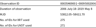
nm) (Poole et al. Reference Poole2007), whereas the X-ray observations were obtained in 0.3–10 keV range. The details of the observations used in the present work are listed in Table 1.
$546.8\pm76.9$
nm) (Poole et al. Reference Poole2007), whereas the X-ray observations were obtained in 0.3–10 keV range. The details of the observations used in the present work are listed in Table 1.
Table 1. Log of observations of Mrk 509 with the Swift observatory.
We extracted light curves in different energy ranges and spectra using the online XRT product generator toolFootnote a. The method used in the online tool is described in Evans et al. (Reference Evans2007); Evans et al. (Reference Evans2009). For generating light curves and spectra, each event file was divided into individual snapshots and further in time intervals for pile-up correction. The source extraction radius is chosen between 11.8 and 70.8 arcsec depending on the mean count rate. The pile-up correction was performed on the time intervals in photon counting (PC) mode where mean count rate is greater than 0.6 counts s–1, by fitting the wings of the source PSF with the King function. For each interval, a source event list and an Ancillary Response File (ARF) were generated and then combined. While combining, each ARF was weighted according to the total counts in the source spectrum extracted from that particular time interval. The background spectrum was extracted by selecting an annular region with inner and outer radii of 142 and 260 arcsec, respectively, within the detector window. Any other source in the background region was excluded from the extraction region. The average count rate was calculated for each observation ID in PC mode of XRT for further timing and spectral analysis of the source.
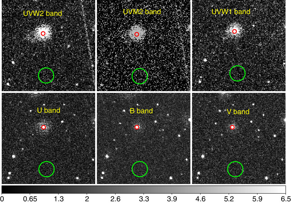
Figure 1. Images of Mrk 509 in six filters of UVOT (marked in each panel) are shown for observation ID : 00035469003. Circular regions of 5 arcsec (red, centred at source position) and 20 arcsec (green, away from the source) radii were selected for the source and background regions, respectively.
Standard procedure was followed to reduce the UVOT data. We used aspect corrected sky image files of each observation ID in every filter to get the average count rate for the selected source region. A circular region of 5 arcsec radius, centred at the source, was selected as the source region to minimise contamination from the host galaxy. For background products, a circular region of 20 arcsec was selected away from the source to avoid contamination from the host galaxy as well as from any other source in the field. The regions selected for the source and background are shown in red and green circles in Figure 1, respectively. The exposures of the UVOT filters are generally in the range of 10 s–2 ks. To get the deepest image, UVOTISUM Footnote b task was used to co-add multiple exposures, if available, in each observation ID. The UVOTSOURCE Footnote c task was used to get the background-corrected source count rate/flux densities in different filters. We also checked for small-scale sensitivity (SSS) regions, where throughput of the detector is comparatively low by running UVOTSOURCE task with additional command lssfile=sssfile5.fits. Apart from this, there are a number of data points where the count rate/flux fall rapidly and show large variability compared to the local mean. This may be due to the bad tracking of the telescope, as described in McHardy et al. (Reference McHardy2014). We discarded those data points from further analysis. We also corrected the count rates to account for the loss of sensitivity of UV detectors with time by using filter correction filesFootnote d.
3. Data analysis and results
3.1. Spectral analysis
The AGNs spectra, especially of Seyferts, in 0.3–10 keV range (the range of operation of Swift/XRT) generally consist of soft X-ray excess and a power law continuum along with the iron emission lines in
 $\sim$
6–7 keV range. In order to investigate the origin of the soft X-ray excess and power law continuum, we carried out spectral analysis using data from all the Swift/XRT observations of Mrk 509. We extracted the time-averaged spectrum of all the observation IDs using the online XRT product generator toolFootnote e (Evans et al. Reference Evans2009). We fitted the spectrum in XSPEC and used C-statistics for minimisation to obtain the best-fit parameters. The errors on each parameter are quoted at 90% confidence level. Using the source and background spectra and appropriate response matrices, we attempted to fit the data in 2–8 keV range with a redshifted power law model along with the multiplicative component tbabs to incorporate the modification due to the Galactic absorption. In our fitting, the Galactic column density was fixed at
$\sim$
6–7 keV range. In order to investigate the origin of the soft X-ray excess and power law continuum, we carried out spectral analysis using data from all the Swift/XRT observations of Mrk 509. We extracted the time-averaged spectrum of all the observation IDs using the online XRT product generator toolFootnote e (Evans et al. Reference Evans2009). We fitted the spectrum in XSPEC and used C-statistics for minimisation to obtain the best-fit parameters. The errors on each parameter are quoted at 90% confidence level. Using the source and background spectra and appropriate response matrices, we attempted to fit the data in 2–8 keV range with a redshifted power law model along with the multiplicative component tbabs to incorporate the modification due to the Galactic absorption. In our fitting, the Galactic column density was fixed at
 $3.95\times10^{20}$
cm–2 (HI4PI Collaboration et al. 2016). The fit statistic was found to be
$3.95\times10^{20}$
cm–2 (HI4PI Collaboration et al. 2016). The fit statistic was found to be
 $C/dof=580.8/597$
for a best-fit power law photon index of
$C/dof=580.8/597$
for a best-fit power law photon index of
 $1.68\pm0.02$
. We extrapolated the fitted model down to 0.3 keV. This showed strong positive residuals in the soft X-ray range (below 1 keV). This confirms the presence of soft X-ray excess in the spectrum. The soft X-ray excess above the power law continuum was fitted with a simple redshifted blackbody (zbbody) model. The positive residuals were still present up to
$1.68\pm0.02$
. We extrapolated the fitted model down to 0.3 keV. This showed strong positive residuals in the soft X-ray range (below 1 keV). This confirms the presence of soft X-ray excess in the spectrum. The soft X-ray excess above the power law continuum was fitted with a simple redshifted blackbody (zbbody) model. The positive residuals were still present up to
 $\sim$
3 keV. We added another redshifted blackbody component to the above model to describe these residuals. The fit statistic improved by
$\sim$
3 keV. We added another redshifted blackbody component to the above model to describe these residuals. The fit statistic improved by
 $\Delta C=-91$
with two additional parameters. The best-fit model tbabs
$\Delta C=-91$
with two additional parameters. The best-fit model tbabs
 $\times$
(zbbody+zbbody+zpowerlaw) resulted in
$\times$
(zbbody+zbbody+zpowerlaw) resulted in
 $C/dof=730.1/764$
. The best-fit value of the power law photon index was found to be
$C/dof=730.1/764$
. The best-fit value of the power law photon index was found to be
 $\Gamma=1.39\pm0.04$
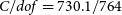
, which is consistent with that reported by Mehdipour et al. (Reference Mehdipour2011). The best-fit model, data and residuals are shown in Figure 2. The best-fitted parameters are given in Table 2.
$\Gamma=1.39\pm0.04$
, which is consistent with that reported by Mehdipour et al. (Reference Mehdipour2011). The best-fit model, data and residuals are shown in Figure 2. The best-fitted parameters are given in Table 2.
Table 2. Best-fit parameters obtained from spectral fitting of Swift/XRT data.

Best-fit model : tbabs
 $\times$
[(zbbody+zbbody+zpowerlw)].
$\times$
[(zbbody+zbbody+zpowerlw)].
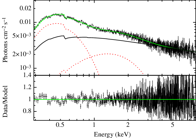
Figure 2. Time-averaged Swift/XRT spectrum of Mrk 509 and best-fit model (green line) are shown along with individual spectral components (red dotted lines for two blackbody components and solid black line for the power law continuum model) in the top panel. Corresponding residuals are shown in the bottom panel.
Following the time-averaged spectroscopy, we attempted to fit the spectra from individual observation IDs with exposures of
 $\sim$
1 ks. Each spectrum was grouped at a minimum of 1 count per bin to use C-statistics in XSPEC spectral fitting. We fitted each spectrum with a simple phenomenological model tbabs
$\sim$
1 ks. Each spectrum was grouped at a minimum of 1 count per bin to use C-statistics in XSPEC spectral fitting. We fitted each spectrum with a simple phenomenological model tbabs
 $\times$
(bbody+zpowerlw) as the second thermal component was not required in fitting. While fitting the spectrum of individual IDs with the above model, we estimated source flux in 0.3–8, 0.3–2, and 2–8 keV ranges for further analysis. The total flux in 0.3–8 keV range, best-fit spectral parameters, and the reduced C for all observation IDs are shown in Figure 3. The variation/non-variation of flux and spectral parameters over the duration of the observations can be clearly seen in the figure. We attempted to search for the presence of any correlation between different parameters obtained from spectral fitting. The correlations between the power law flux (in 2–8 keV range), blackbody flux (BB flux in 0.3–2 keV range), power law photon index, and blackbody temperature are shown in Figure 4. From this analysis, we found a moderate correlation between the blackbody flux and power law flux with Pearson’s coefficient
$\times$
(bbody+zpowerlw) as the second thermal component was not required in fitting. While fitting the spectrum of individual IDs with the above model, we estimated source flux in 0.3–8, 0.3–2, and 2–8 keV ranges for further analysis. The total flux in 0.3–8 keV range, best-fit spectral parameters, and the reduced C for all observation IDs are shown in Figure 3. The variation/non-variation of flux and spectral parameters over the duration of the observations can be clearly seen in the figure. We attempted to search for the presence of any correlation between different parameters obtained from spectral fitting. The correlations between the power law flux (in 2–8 keV range), blackbody flux (BB flux in 0.3–2 keV range), power law photon index, and blackbody temperature are shown in Figure 4. From this analysis, we found a moderate correlation between the blackbody flux and power law flux with Pearson’s coefficient
 $\rho\,{\sim}\,0.56$
, between the blackbody temperature and blackbody flux with
$\rho\,{\sim}\,0.56$
, between the blackbody temperature and blackbody flux with
 $\rho\sim0.31$
, and between the blackbody temperature and photon index with
$\rho\sim0.31$
, and between the blackbody temperature and photon index with
 $\rho\sim-0.38$
. Considering the narrow energy range of XRT and short exposure of observations, there is a possibility of presence of degeneracy between parameters. Therefore, we investigated the marginal posterior distributions of all the fitted parameters to determine the degree to which the parameters are correlated due to the degeneracies within the spectral fitting. In order to search through the parameter space, the data from the observation with maximum exposure, i.e.,
$\rho\sim-0.38$
. Considering the narrow energy range of XRT and short exposure of observations, there is a possibility of presence of degeneracy between parameters. Therefore, we investigated the marginal posterior distributions of all the fitted parameters to determine the degree to which the parameters are correlated due to the degeneracies within the spectral fitting. In order to search through the parameter space, the data from the observation with maximum exposure, i.e.,
 $\sim$
7 ks (Obs. ID 00035469003) were used for fitting by applying the Markov Chain Monte Carlo (MCMC) sampling procedure. We used the affine-invariant sampler developed by Goodman & Weare (Reference Goodman and Weare2010) and implemented in XSPEC as CHAIN task. For tbabs
$\sim$
7 ks (Obs. ID 00035469003) were used for fitting by applying the Markov Chain Monte Carlo (MCMC) sampling procedure. We used the affine-invariant sampler developed by Goodman & Weare (Reference Goodman and Weare2010) and implemented in XSPEC as CHAIN task. For tbabs
 $\times$
(zbbody+zpowerlw) model, we considered 20 walkers with a total chain length of 100000 and burning initial steps of 20000. In Figure 6, we showed one- and two-dimensional (1D and 2D) marginal posterior distributions for the spectral parameters. The median values of the parameters with 90% credible interval are shown above each 1D histogram. The Pearson’s correlation coefficients for these distributions are
$\times$
(zbbody+zpowerlw) model, we considered 20 walkers with a total chain length of 100000 and burning initial steps of 20000. In Figure 6, we showed one- and two-dimensional (1D and 2D) marginal posterior distributions for the spectral parameters. The median values of the parameters with 90% credible interval are shown above each 1D histogram. The Pearson’s correlation coefficients for these distributions are
 $-0.26$
for kT
$-0.26$
for kT
 $_{\rm BB}$
and kT
$_{\rm BB}$
and kT
 $_{\rm norm}$
,
$_{\rm norm}$
,
 $-0.49$
for
$-0.49$
for
 $\Gamma$
and kT
$\Gamma$
and kT
 $_{\rm BB}$
,
$_{\rm BB}$
,
 $-0.47$
for
$-0.47$
for
 $\Gamma$
and kT
$\Gamma$
and kT
 $_{\rm norm}$
,
$_{\rm norm}$
,
 $-0.59$
for
$-0.59$
for
 $\Gamma_{\rm norm}$
and kT
$\Gamma_{\rm norm}$
and kT
 $_{\rm BB}$
,
$_{\rm BB}$
,
 $-0.44$
for
$-0.44$
for
 $\Gamma_{\rm norm}$
and kT
$\Gamma_{\rm norm}$
and kT
 $_{\rm norm}$
, and
$_{\rm norm}$
, and
 $0.85$
for
$0.85$
for
 $\Gamma_{\rm norm}$
and
$\Gamma_{\rm norm}$
and
 $\Gamma$
with p-value <
$\Gamma$
with p-value <
 $10^{-5}$
. It is evident from the figure that the correlation between the blackbody temperature and the photon index is not physical, instead spurious. On a careful investigation of correlation between spectral parameters from spectral fitting of all the observations and the MCMC sampling procedure, it is confirmed that there exists a certain degree of degeneracy between power law photon index and blackbody temperature. However, the narrow energy range of Swift/XRT and short exposure time (
$10^{-5}$
. It is evident from the figure that the correlation between the blackbody temperature and the photon index is not physical, instead spurious. On a careful investigation of correlation between spectral parameters from spectral fitting of all the observations and the MCMC sampling procedure, it is confirmed that there exists a certain degree of degeneracy between power law photon index and blackbody temperature. However, the narrow energy range of Swift/XRT and short exposure time (
 ${\sim}$
1 ks) of individual observations make it extremely difficult to remove this degeneracy through spectral fitting. Considering this, we proceeded with time series analysis using data from all the Swift/XRT observations.
${\sim}$
1 ks) of individual observations make it extremely difficult to remove this degeneracy through spectral fitting. Considering this, we proceeded with time series analysis using data from all the Swift/XRT observations.
Figure 3. Variation of the source flux in 0.3–8 keV range, blackbody temperature (kT), and power law photon index (
 $\Gamma$
) with time (MJD) are shown in top three panels. The reduced C-stat obtained from the spectral fitting of each observation ID is plotted in the bottom panel.
$\Gamma$
) with time (MJD) are shown in top three panels. The reduced C-stat obtained from the spectral fitting of each observation ID is plotted in the bottom panel.

Figure 4. Pearson’s correlation coefficients (
 $\rho, p$
-value) between different spectral parameters extracted from fitting of individual observations using phenomenological model tbabs
$\rho, p$
-value) between different spectral parameters extracted from fitting of individual observations using phenomenological model tbabs
 $\times$
[bbody+zpowerlw]. The 0.3–2 keV blackbody flux (F
$\times$
[bbody+zpowerlw]. The 0.3–2 keV blackbody flux (F
 $_{BB}$
; in units of 10–11 erg s–1 cm–2) has been plotted against 2–8 keV power law flux (F
$_{BB}$
; in units of 10–11 erg s–1 cm–2) has been plotted against 2–8 keV power law flux (F
 $_{PL}$
; in units of 10–11 erg s–1 cm–2), photon index (
$_{PL}$
; in units of 10–11 erg s–1 cm–2), photon index (
 $\Gamma$
), and blackbody temperature KT
$\Gamma$
), and blackbody temperature KT
 $_{BB}$
(in unit of keV) from top to bottom, respectively, in the left panels of the figure. In the right panels, the plots for
$_{BB}$
(in unit of keV) from top to bottom, respectively, in the left panels of the figure. In the right panels, the plots for
 $\Gamma$
versus KT
$\Gamma$
versus KT
 $_{BB}$
and
$_{BB}$
and
 $\Gamma$
versus F
$\Gamma$
versus F
 $_{PL}$
have been shown.
$_{PL}$
have been shown.
3.2. Timing analysis
3.2.1. Variability amplitudes and nature of variability
As described in Section 2, the source flux densities for all six UVOT filters were estimated from all observation IDs. Soft X-ray (0.3–2 keV range) and hard X-ray (2–8 keV) fluxes were estimated from spectral analysis of Swift/XRT data of each observation ID (see Section 3.1). Using these estimated flux densities, simultaneous X-ray and UVOT light curves of Mrk 509 for the duration of the Swift monitoring campaign, i.e., from 2006 June 18 to 2019 May 8, are generated and shown in Figure 5. It can be clearly seen that the light curves in different bands show variabilities in short-term as well as long-term timescales. To quantify the observed variabilities in X-ray and UV/optical light curves, we calculated fractional variability
 $F_{var}$
and its uncertainty using the relations,
$F_{var}$
and its uncertainty using the relations,
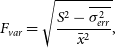 $${F_{var}} = \sqrt {{{{S^2} - \overline {\sigma _{err}^2} } \over {{{\bar x}^2}}}} ,$$
and uncertainty in
 $F_{var}$
,
$F_{var}$
,
 \begin{equation*}\sqrt{\Bigg( \sqrt{\frac{1}{2N}} \frac{\overline{\sigma^2_{err}}}{\bar{x}^2 F_{var}} \Bigg)^2 + \Bigg( \sqrt{\frac{\overline{\sigma^2_{err}}}{N}} \frac{1}{\bar{x}}\Bigg)^2 },\end{equation*}
where
 $\bar{x}$
, S,
$\bar{x}$
, S,
 $\overline{\sigma}_{err}$
, and N are the mean, total variance, mean error, and number of data points, respectively (Vaughan et al. Reference Vaughan, Edelson, Warwick and Uttley2003), for X-ray and UV/optical bands. Using the above expressions, the fractional variabilities in hard X-ray (2–8 keV), soft X-ray (0.3–2 keV), UVW2, UVM2, UVW1, U, B, and V bands are derived to be
$\overline{\sigma}_{err}$
, and N are the mean, total variance, mean error, and number of data points, respectively (Vaughan et al. Reference Vaughan, Edelson, Warwick and Uttley2003), for X-ray and UV/optical bands. Using the above expressions, the fractional variabilities in hard X-ray (2–8 keV), soft X-ray (0.3–2 keV), UVW2, UVM2, UVW1, U, B, and V bands are derived to be
 $0.152\pm0.010$
,
$0.152\pm0.010$
,
 $0.281\pm0.006$
,
$0.281\pm0.006$
,
 $0.223\pm0.001$
,
$0.223\pm0.001$
,
 $0.234\pm0.002$
,
$0.234\pm0.002$
,
 $0.184\pm0.002$
,
$0.184\pm0.002$
,
 $0.174\pm0.002$
,
$0.174\pm0.002$
,
 $0.147\pm0.002$
, and
$0.147\pm0.002$
, and
 $0.114\pm0.002$
, respectively. Within the UV/optical bands, the variability amplitudes are found to decrease with the increase in wavelength. This trend has been reported in many previous studies (Fausnaugh et al. Reference Fausnaugh2016; Edelson et al. Reference Edelson2019) as emission at longer wavelengths is expected to originate from regions in accretion disk at larger radii and thus, prone to dilute with other effects like emission from BLR and narrow-line region (NLR) or host galaxy. From the spectral analysis, we found a complex soft X-ray excess described by two thermal components. Thus, high variability in the soft X-ray band could be due to a mixture of different spectral components, i.e., thermal plasma in the inner disk, X-ray reprocessing close to the inner edge of the disk. Since the signatures of warm absorbers have already been reported in previous studies (Ebrero et al. Reference Ebrero2011; Steenbrugge et al. Reference Steenbrugge2011), and we see some residuals below 1 keV (Figure 2), variability due to the warm absorbers cannot be ruled out.
$0.114\pm0.002$
, respectively. Within the UV/optical bands, the variability amplitudes are found to decrease with the increase in wavelength. This trend has been reported in many previous studies (Fausnaugh et al. Reference Fausnaugh2016; Edelson et al. Reference Edelson2019) as emission at longer wavelengths is expected to originate from regions in accretion disk at larger radii and thus, prone to dilute with other effects like emission from BLR and narrow-line region (NLR) or host galaxy. From the spectral analysis, we found a complex soft X-ray excess described by two thermal components. Thus, high variability in the soft X-ray band could be due to a mixture of different spectral components, i.e., thermal plasma in the inner disk, X-ray reprocessing close to the inner edge of the disk. Since the signatures of warm absorbers have already been reported in previous studies (Ebrero et al. Reference Ebrero2011; Steenbrugge et al. Reference Steenbrugge2011), and we see some residuals below 1 keV (Figure 2), variability due to the warm absorbers cannot be ruled out.
Based on the probability spectral density (PSD) studies, the nature of variability in AGNs is considered to be red noise variability (Papadakis & Lawrence Reference Papadakis and Lawrence1993). This is very similar to the one that is observed in Galactic black holes, where the PSD is described by a broken power law at a specific frequency depending on the spectral state. Switching between different states indicates that the variability process is non-stationary. Statistically, in non-stationary process, the moments of the probability distribution function (i.e., mean and variance) vary with time. In the left panel of Figure 7, we plotted the change of mean
 $< x > $
, excess variance
$< x > $
, excess variance
 $\sigma^2_{xs}$
and fractional rms amplitude
$\sigma^2_{xs}$
and fractional rms amplitude
 $F_{var}$
(computed by taking 10 data points) in 0.3–10 keV light curve with time. All these quantities are found to change with time. In the bottom panel, the averaged rms has been shown (binned over 5 data points of individual rms), which also changes with time, indicating the non-stationarity of the variability process. We divided the entire light curve into two segments covering the time from 57829 to 57967 MJD and 57968 to 58102 MJD, respectively, (marked with a dotted line in the top left panel of Figure 7) and calculated the autocorrelation function (ACF) of each segment (Gliozzi et al. Reference Gliozzi, Papadakis, Sambruna and Eracleous2004). The rate at which the ACF decays for each segment is different. This suggests that there is an intrinsic difference in the temporal properties in both segments. This indicates non-stationary variability, though we cannot claim it firmly due to the quality of the data used. We also did not find any signature of apparent state change over the duration of the observations (see Figure 3).
$F_{var}$
(computed by taking 10 data points) in 0.3–10 keV light curve with time. All these quantities are found to change with time. In the bottom panel, the averaged rms has been shown (binned over 5 data points of individual rms), which also changes with time, indicating the non-stationarity of the variability process. We divided the entire light curve into two segments covering the time from 57829 to 57967 MJD and 57968 to 58102 MJD, respectively, (marked with a dotted line in the top left panel of Figure 7) and calculated the autocorrelation function (ACF) of each segment (Gliozzi et al. Reference Gliozzi, Papadakis, Sambruna and Eracleous2004). The rate at which the ACF decays for each segment is different. This suggests that there is an intrinsic difference in the temporal properties in both segments. This indicates non-stationary variability, though we cannot claim it firmly due to the quality of the data used. We also did not find any signature of apparent state change over the duration of the observations (see Figure 3).
3.2.2. Count–Count Correlation with Positive Offset (C3PO)
We defined
 $0.3{-}2$
keV and
$0.3{-}2$
keV and
 $2{-}8$
keV energy ranges as soft and hard X-ray bands. The soft X-ray band have several complex features such as soft X-ray excess, emission lines, blurred reflection, and absorption features, while the hard band is mainly dominated by primary continuum resulted from multiple inverse Compton scattering of seed photons with electron plasma in the corona. We plotted light curves in soft X-ray band, hard X-ray band, and all the filters of optical and UV bands in Figure 5. From visual inspection, all the light curves seem to be correlated. The variations in UV/optical bands are smoother than the X-rays.
$2{-}8$
keV energy ranges as soft and hard X-ray bands. The soft X-ray band have several complex features such as soft X-ray excess, emission lines, blurred reflection, and absorption features, while the hard band is mainly dominated by primary continuum resulted from multiple inverse Compton scattering of seed photons with electron plasma in the corona. We plotted light curves in soft X-ray band, hard X-ray band, and all the filters of optical and UV bands in Figure 5. From visual inspection, all the light curves seem to be correlated. The variations in UV/optical bands are smoother than the X-rays.
We attempted to quantify the correlations and variabilities seen in UV/optical and X-ray light curves using C3PO method. The C3PO method was first used by Churazov et al. (Reference Churazov, Gilfanov and Revnivtsev2001) in the black hole binary system Cygnus X-1 to find the varying and stable components in high/soft state. After that, this technique has been used in many AGNs (Taylor et al. Reference Taylor, Uttley and McHardy2003; Noda et al. Reference Noda, Makishima, Yamada, Torii, Sakurai and Nakazawa2011; Reference Noda, Makishima, Nakazawa and Yamada2013; Reference Noda2016; Pal & Naik Reference Pal and Naik2017). We fitted a linear function
 $y=mx+c$
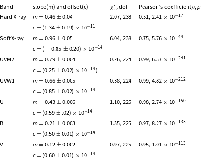
between the reference band as abscissa and secondary bands as ordinate, where m and c are the slope and offset, respectively. In the left and right panels of Figure 8, the hard X-ray (2–8 keV) and UVW2 bands are taken as reference bands, respectively, and all other bands are considered as secondary. For uniformity, the plots have been shown for flux densities though there was no difference in the fitted values when plotted in count rates. We also used Pearson’s correlation coefficient ‘
$y=mx+c$
between the reference band as abscissa and secondary bands as ordinate, where m and c are the slope and offset, respectively. In the left and right panels of Figure 8, the hard X-ray (2–8 keV) and UVW2 bands are taken as reference bands, respectively, and all other bands are considered as secondary. For uniformity, the plots have been shown for flux densities though there was no difference in the fitted values when plotted in count rates. We also used Pearson’s correlation coefficient ‘
 $\rho$
’ to quantify the strength of inter-band correlation and determined the significance of the strength of the correlation. All the values of slopes, offset, Pearson’s coefficient are given in Tables 3 and 4. From the linear fitting, we found a reasonable correlation between hard X-rays and all UV/optical bands (
$\rho$
’ to quantify the strength of inter-band correlation and determined the significance of the strength of the correlation. All the values of slopes, offset, Pearson’s coefficient are given in Tables 3 and 4. From the linear fitting, we found a reasonable correlation between hard X-rays and all UV/optical bands (
 $\rho\ \sim\ 0.40{-}0.53$
). However, the correlation between the UVW2 and other UV–optical bands is found to be stronger (
$\rho\ \sim\ 0.40{-}0.53$
). However, the correlation between the UVW2 and other UV–optical bands is found to be stronger (
 $\rho\,{\sim}\,0.95{-}0.99$
). When fitted relative to UVW2 band, a positive offset (except for soft X-rays) has been found for all other UV/optical bands, including hard X-ray. This indicates that the less variable component is possibly coming from the BLR and the host galaxy. Similar results have been drawn from the flux–flux analysis for other systems, e.g., Fairall 9 (Hernandez Santisteban et al. Reference Hernandez Santisteban2020).
$\rho\,{\sim}\,0.95{-}0.99$
). When fitted relative to UVW2 band, a positive offset (except for soft X-rays) has been found for all other UV/optical bands, including hard X-ray. This indicates that the less variable component is possibly coming from the BLR and the host galaxy. Similar results have been drawn from the flux–flux analysis for other systems, e.g., Fairall 9 (Hernandez Santisteban et al. Reference Hernandez Santisteban2020).
Table 3. Slope, offset, and Pearson’s coefficient for hard X-ray versus soft bands (soft X-ray and UV/optical bands).
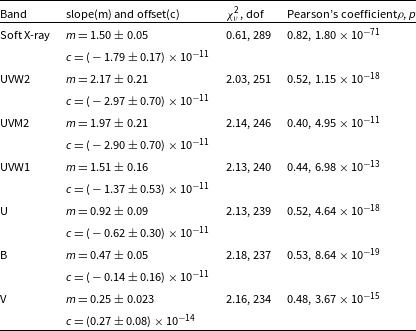
Table 4. Slope, offset, and Pearson’s coefficient for UVW2 versus other UV/optical bands.
3.2.3. Filtering of slow and linear variations
To understand the short-term variabilities in different bands due to reprocessing, i.e., X-ray reprocessing or Comptonizaton, we focused on the fast variations in the light curves. It is well known that the long-term variations can distort the short-term time lags while estimating CCFs (Welsh Reference Welsh1999). So we attempted to remove the slow variations, i.e., long-term variations due to the changes in the accretion rate, from the light curves. As mentioned above, Figure 5 shows short-term variations as well as long-term variations in the curves in all bands. Therefore, the long-term variations should be filtered out from the light curves to determine short time information. Such filtering has been carried out in recent studies in a few AGNs, e.g., NGC 5548 (McHardy et al. Reference McHardy2014), NGC 4593 (McHardy et al. Reference McHardy2018), NGC 7469 (Pahari et al. Reference Pahari, McHardy, Vincentelli, Cackett, Peterson, Goad, Gültekin and Horne2020), to eliminate the effect of long-term variations. We used the locally weighted scatter smoothing (LOWESS) method for the filtering process, which is based on non-parametric and non-linear least square regression method (Cleveland & Devlin Reference Cleveland and Devlin1988). In this method, a regression surface is estimated by fitting a low-degree polynomial locally to a subset of the data. The polynomial is fitted with weighted least squares, giving more weight to the near data points and least weight to the farthest ones. The tricube function,
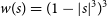 $w(s)=(1-{\lvert s \rvert}^3)^3$
is used to calculate the weight, where s is the distance of a given data point from the neighbouring point scaled to lie in the range of 0–1. Here,
$w(s)=(1-{\lvert s \rvert}^3)^3$
is used to calculate the weight, where s is the distance of a given data point from the neighbouring point scaled to lie in the range of 0–1. Here,
 $s(t)=(t-t_i/\Delta t)$
is the time difference between time t and
$s(t)=(t-t_i/\Delta t)$
is the time difference between time t and
 $t_i$
at the data point i in terms of filtering time
$t_i$
at the data point i in terms of filtering time
 $\Delta t$
. For this work, we used different filtering time to calculate the time lags as well as to investigate the effect of filtering of the long-term variations. Since the filtering process has a limitation that it can only be performed on densely populated sample, we, therefore, applied the LOWESS filtering to the data in the range of MJD 57829–MJD 58102 and calculated the time lags.
$\Delta t$
. For this work, we used different filtering time to calculate the time lags as well as to investigate the effect of filtering of the long-term variations. Since the filtering process has a limitation that it can only be performed on densely populated sample, we, therefore, applied the LOWESS filtering to the data in the range of MJD 57829–MJD 58102 and calculated the time lags.
We filtered out the slow variations of the order of more than 10, 15, 18, 20, and 25 days from all light curves shown in Figure 5. Although the average cadence of the observations was about 1 day, filtering for less than 10 days was not feasible due to the gap of 6 days between two observations. Filtered light curves for the UVW2 and UVW1 bands, after removing slow variations of the order of 20 days, are shown in Figure 9 (left panels).
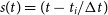
For determining the short time delay between two filtered light curves, we applied ICCF method (described in detail in Section 3.2.4). The estimated time delays between UVW2 and other bands after filtering have been listed in Table 5. The CCF lag distribution for 20 days filtering and without filtering have been plotted in the right panel of Figure 9 to compare the effect of filtering on CCF distribution. It can be seen from the figure that after filtering, the distribution is significantly narrower than the unfiltered one. This indicates that the slower variations were causing the wider CCF which became narrower after filtering the long-term variations from the light curves. The derived lags of X-ray emission with respect to the UVW2 emission from the unfiltered and filtered light curves clearly show the effect of the removal of slow variations (see Table 5). Further, to check the effect of different filtering amongst UV and optical bands, we filtered slow variations for different days from all the light curves and estimated time lags with respect to the UVW2 band.
Table 5. Time lags (in days) in different energy band relative to the UVW2 band estimated from the ICCF correlation method.
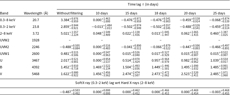

Figure 5. Simultaneous UV/optical and X-ray light curves of Mrk 509 from Swift observations during 2006 June 18–2019 May 8. The UV/optical (UVW2, UVM2, UVW1, U, B, V) flux densities (in 10–14 erg s–1 cm–2 Å–1) of the source are plotted with the hard X-ray (2–8 keV) and soft X-ray (0.3–2 keV) flux densities (10–11 erg s–1 cm–2). The X-ray flux densities were estimated from spectral fitting of data from the individual observation IDs. Two breaks in the light curves are due to the large observation gaps.

Figure 6. 1D and 2D marginal posterior distributions for power law photon index (
 $\Gamma$
) and its normalisation (
$\Gamma$
) and its normalisation (
 $\Gamma_{norm}$
), blackbody temperature (
$\Gamma_{norm}$
), blackbody temperature (
 $kT_{BB}$
, in keV) and its normalisation (
$kT_{BB}$
, in keV) and its normalisation (
 $kT_{norm}$
) for Obs. ID 00035469003 fitted with tbabs
$kT_{norm}$
) for Obs. ID 00035469003 fitted with tbabs
 $\times$
[bbody+zpowerlw] model. Vertical lines in 1D distributions show 16%, 50%, and 90% quantiles. CORNER.PY (Foreman-Mackey Reference Foreman-Mackey2016) was used to plot these distributions.
$\times$
[bbody+zpowerlw] model. Vertical lines in 1D distributions show 16%, 50%, and 90% quantiles. CORNER.PY (Foreman-Mackey Reference Foreman-Mackey2016) was used to plot these distributions.
Figure 7. Left panel: Light curve of Mrk 509 in 0.3–10 keV range is shown in the top panel. The mean count rate, excess variance, and fractional rms amplitude measured from the segment of 10 points are shown in the second, third, and fourth panels from top. In the bottom panel, averaged fractional rms amplitude is shown by binning five amplitudes. Right panel : Autocorrelations calculated for two segments (from 57829 to 57967 MJD and 57968 to 58102 MJD, as marked with a dotted line in the top left panel) of 0.3–10 keV light curves are shown.

Figure 8. C3PO plots are shown for hard X-ray band (left panels) and UVW2 band (right panels) as reference bands. The best-fitted linear equations are presented as red solid lines. The units of the fluxes are 10–11 erg s–1 cm–2 for X-ray bands and 10–14 erg s–1 cm–2 Å–1 for UV/optical bands.
3.2.4. Time lag estimation
After removing the slow variations from the observed light curves, we measured the lags in different bands with respect to the UVW2 band. For the estimation of time lags, we used two methods that are interpolation cross-correlation function (ICCF; Gaskell & Peterson Reference Gaskell and Peterson1987, Peterson et al. Reference Peterson, Wanders, Horne, Collier, Alexander, Kaspi and Maoz1998) and JAVELIN (Zu et al. Reference Zu, Kochanek and Peterson2011). The lags estimated using these two methods were similar except that the errors calculated from JAVELIN were smaller, as previously noted by Fausnaugh et al. Reference Fausnaugh2016. In the ICCF method, we assume that two light curves, say a(t) and b(t) are displaced by a time lag of
 $\tau$
. First, each observed data point of the curve b(t) is correlated with a linearly interpolated value of a(t) at a time difference of
$\tau$
. First, each observed data point of the curve b(t) is correlated with a linearly interpolated value of a(t) at a time difference of
 $\tau$
. Similarly, each observed data point in curve a(t) is correlated with an interpolated value in b(t). In this way, two correlation coefficients are calculated for each value of time lag
$\tau$
. Similarly, each observed data point in curve a(t) is correlated with an interpolated value in b(t). In this way, two correlation coefficients are calculated for each value of time lag
 $\tau$
and then averaged out to get the final value of the correlation coefficient. Uncertainties on the lag measurements are estimated using flux randomisation (FR) and random subset selection (RSS) methods. In the RSS method, the N selections are drawn randomly from the light curve of N data points for each Monte Carlo realisation, similar to the bootstraping method. The data point which is selected M times, the uncertainty is decreased by
$\tau$
and then averaged out to get the final value of the correlation coefficient. Uncertainties on the lag measurements are estimated using flux randomisation (FR) and random subset selection (RSS) methods. In the RSS method, the N selections are drawn randomly from the light curve of N data points for each Monte Carlo realisation, similar to the bootstraping method. The data point which is selected M times, the uncertainty is decreased by
 $M^{1/2}$
. To assess the flux uncertainty, the random Gaussian deviates are added to the data points (FR). After multiple Monte Carlo realisations, a cross-correlation function is obtained having correlation coefficient at the peak and centroid lags (usually measured above the 80% of peak value). The peak and centroid lag values differ for asymmetric ICCF distribution. We performed 2000 Monte Carlo simulations for each pair of light curves of UVW2 and other bands and rejected those cross-correlation coefficients that were below 0.2. Time lags calculated with and without filtering have been tabulated in Table 5. Edelson et al. (Reference Edelson2019) calculated time lags using average count rates in the light curves for this source without removing any slow variations which are found to be consistent with the values reported in the present work (within error). However, there is a difference in the centroid value of lags in UVM2 and UVW1.
$M^{1/2}$
. To assess the flux uncertainty, the random Gaussian deviates are added to the data points (FR). After multiple Monte Carlo realisations, a cross-correlation function is obtained having correlation coefficient at the peak and centroid lags (usually measured above the 80% of peak value). The peak and centroid lag values differ for asymmetric ICCF distribution. We performed 2000 Monte Carlo simulations for each pair of light curves of UVW2 and other bands and rejected those cross-correlation coefficients that were below 0.2. Time lags calculated with and without filtering have been tabulated in Table 5. Edelson et al. (Reference Edelson2019) calculated time lags using average count rates in the light curves for this source without removing any slow variations which are found to be consistent with the values reported in the present work (within error). However, there is a difference in the centroid value of lags in UVM2 and UVW1.
We also applied JAVELIN method to calculate the inter-band lags. Instead of linearly interpolating between the gaps, JAVELIN models the light curves by making an assumption that the driving light curve is modelled by a damped random walk (DRW) that has been generally applied in quasars (Zu et al. Reference Zu, Kochanek, Kozłowski and Udalski2013) and the derived light curves are related to the driving light curve via a top-hat transfer function. This method was first applied by Kelly et al. (Reference Kelly, Bechtold and Siemiginowska2009). The time lags for X-rays, UVM2, UVW1, U, B, V bands relative to UVW2 band, without filtering are
 $-2.086\pm3.041$
,
$-2.086\pm3.041$
,
 $-0.311\pm0.218$
,
$-0.311\pm0.218$
,
 $0.132\pm0.196$
,
$0.132\pm0.196$
,
 $1.656\pm0.337$
,
$1.656\pm0.337$
,
 $1.298\pm0.404$
, and
$1.298\pm0.404$
, and
 $2.458\pm0.607$
, respectively. After 20 days filtering, these lags were found to be
$2.458\pm0.607$
, respectively. After 20 days filtering, these lags were found to be
 $-1.232\pm0.509$
,
$-1.232\pm0.509$
,
 $-0.123\pm0.239$
,
$-0.123\pm0.239$
,
 $-0.023\pm0.266$
,
$-0.023\pm0.266$
,
 $0.729\pm0.488$
,
$0.729\pm0.488$
,
 $1.086\pm0.639$
, and
$1.086\pm0.639$
, and
 $2.474\pm1.246$
, respectively. These lags are consistent with that found with the ICCF method.
$2.474\pm1.246$
, respectively. These lags are consistent with that found with the ICCF method.
We derived the lag spectrum, i.e., lag as a function of wavelength for unfiltered and filtered (for 18 days filtering) light curves and showed it in the left and right panels of Figure 10, respectively. We then used a phenomenological power law model to model the lag spectrum. An expression of such power law model in terms of lags, i.e., the time delay between a reference wavelength (
 $\lambda_0$
) and other wavelength (
$\lambda_0$
) and other wavelength (
 $\lambda$
) can be given as
$\lambda$
) can be given as
 \begin{equation*}\tau=\alpha \left[ \left( \frac{\lambda}{\lambda_0} \right)^{\beta} -1 \right],\end{equation*}
where
 $\tau$
,
$\tau$
,
 $\alpha$
, and
$\alpha$
, and
 $\beta$
are time delay between reprocessing and reprocessed emission, power law normalisation, and power law index, respectively. In the standard accretion disk theory, the value of power law index
$\beta$
are time delay between reprocessing and reprocessed emission, power law normalisation, and power law index, respectively. In the standard accretion disk theory, the value of power law index
 $\beta$
is considered to be 4/3 (Collier et al. Reference Collier, Horne, Wanders and Peterson1999; Cackett et al. Reference Cackett, Horne and Winkler2007). We modelled the lag spectrum with the power law model in the following ways: (a) varying normalisation
$\beta$
is considered to be 4/3 (Collier et al. Reference Collier, Horne, Wanders and Peterson1999; Cackett et al. Reference Cackett, Horne and Winkler2007). We modelled the lag spectrum with the power law model in the following ways: (a) varying normalisation
 $\alpha$
and power law index
$\alpha$
and power law index
 $\beta$
with and without hard and soft X-ray lags and (b) by fixing the value of
$\beta$
with and without hard and soft X-ray lags and (b) by fixing the value of
 $\beta$
as
$\beta$
as
 $4/3$
and varying normalisation only. Since there was an excess lag in U band for unfiltered case, it was removed from the lag spectrum. Here, the UVW2 band is considered as the reference waveband. The parameters obtained from fitting the lag spectrum for unfiltered light curves are (a)
$4/3$
and varying normalisation only. Since there was an excess lag in U band for unfiltered case, it was removed from the lag spectrum. Here, the UVW2 band is considered as the reference waveband. The parameters obtained from fitting the lag spectrum for unfiltered light curves are (a)
 $\alpha$
= 0.14
$\alpha$
= 0.14
 $\pm$
0.75,
$\pm$
0.75,
 $\beta$
= 2.71
$\beta$
= 2.71
 $\pm$
5.08 (including all the wavebands), and
$\pm$
5.08 (including all the wavebands), and
 $\alpha$
= 1.49
$\alpha$
= 1.49
 $\pm$
5.71
$\pm$
5.71
 $\beta$
= 0.78
$\beta$
= 0.78
 $\pm$
2.11 (excluding X-ray and U bands) and (b)
$\pm$
2.11 (excluding X-ray and U bands) and (b)
 $\alpha$
= 0.51
$\alpha$
= 0.51
 $\pm$
0.44. After 18 days filtering of light curves, the parameters are (a)
$\pm$
0.44. After 18 days filtering of light curves, the parameters are (a)
 $\alpha$
= 0.26
$\alpha$
= 0.26
 $\pm$
0.15,
$\pm$
0.15,
 $\beta$
= 2.28
$\beta$
= 2.28
 $\pm$
0.59 (including all wavebands),
$\pm$
0.59 (including all wavebands),
 $\alpha$
= 0.20
$\alpha$
= 0.20
 $\pm$
0.19,
$\pm$
0.19,
 $\beta$
= 2.52
$\beta$
= 2.52
 $\pm$
0.98 (excluding X-ray bands) and (b)
$\pm$
0.98 (excluding X-ray bands) and (b)
 $\alpha$
= 0.61
$\alpha$
= 0.61
 $\pm$
0.12. The lag spectrum along with fitted power law models (as described above) without filtering and 18 days filtering of light curves are shown in the left and right panels of Figure 10, respectively. From the figure, it is clear that there is a large discrepancy between the model and observed lag even after filtering the light curves for long-term variations.
$\pm$
0.12. The lag spectrum along with fitted power law models (as described above) without filtering and 18 days filtering of light curves are shown in the left and right panels of Figure 10, respectively. From the figure, it is clear that there is a large discrepancy between the model and observed lag even after filtering the light curves for long-term variations.
4. Discussion
4.1. Correlations observed in the X-ray and UV/optical emission
From the analysis, we found that the average spectrum over a duration of 13 years shows the presence of a complicated soft X-ray excess over the power law continuum. The soft X-ray excess is described well with a combination of two thermal components with temperatures of
 $kT_{\rm BB1}\sim 120$
eV and
$kT_{\rm BB1}\sim 120$
eV and
 $kT_{\rm BB2}\sim 460$
eV. The low-temperature thermal component is normally required in Seyfert 1 AGNs (Leighly Reference Leighly1999). However, the warm thermal component may be an analogy to the warm Comptonization, as described by Done et al. (Reference Done, Davis, Jin, Blaes and Ward2012), to explain the soft X-ray excess. According to this model, the warm Comptonizing plasma (
$kT_{\rm BB2}\sim 460$
eV. The low-temperature thermal component is normally required in Seyfert 1 AGNs (Leighly Reference Leighly1999). However, the warm thermal component may be an analogy to the warm Comptonization, as described by Done et al. (Reference Done, Davis, Jin, Blaes and Ward2012), to explain the soft X-ray excess. According to this model, the warm Comptonizing plasma (
 ${\sim}0.2{-}0.5$
keV) is embedded inside the optically thin and hot Comptonizing plasma (
${\sim}0.2{-}0.5$
keV) is embedded inside the optically thin and hot Comptonizing plasma (
 ${\sim}100$
keV). The soft X-ray excess due to warm Comptonization was also reported in this AGN by Mehdipour et al. (Reference Mehdipour2011). Such a geometry of disk/X-ray plasma may be supported due to the observed correlation between the soft X-ray and hard X-ray emission (
${\sim}100$
keV). The soft X-ray excess due to warm Comptonization was also reported in this AGN by Mehdipour et al. (Reference Mehdipour2011). Such a geometry of disk/X-ray plasma may be supported due to the observed correlation between the soft X-ray and hard X-ray emission (
 $\rho\sim0.82$
, log
$\rho\sim0.82$
, log
 $p \sim-71$
). In that case, the variability amplitude observed in the UV and soft X-ray bands should be, at least, equal to that of the highly variable power law continuum flux. From the estimation of fractional variability, we found a low variability amplitude of the power law continuum flux (
$p \sim-71$
). In that case, the variability amplitude observed in the UV and soft X-ray bands should be, at least, equal to that of the highly variable power law continuum flux. From the estimation of fractional variability, we found a low variability amplitude of the power law continuum flux (
 ${\sim}15\%$
). This suggests that the hot X-ray plasma may not be lying over the warm Comptonizing plasma, but situated at a different location closer to the SMBH. Further, the correlation between the derived spectral components such as power law flux and BB flux and BB temperature and BB flux are weak or moderate while other combinations do not show any correlation (see Figure 4). The observed weak anti-correlation between the power law photon index and blackbody temperature, though both the components overlap only in a narrow energy range (below 2 keV), is apparently due to the degeneracy between both the parameters. Therefore, the emitting regions are likely to be partly interacting or distinct. At the same time, the variability observed in the UV emission, which is supposed to be radiated from regions close to the SMBH as compared to the optical emission, is also higher than that observed in the hard X-ray emission. However, the hard X-ray emission variability is higher relative to the changes found in the V band. This also suggests that the UV and hard X-ray emission may be associated with disjoint regions or partly interacting regions. Similarly, the C3PO analysis gives a negative offset for the soft X-ray and UV/optical bands (except the V band) while taking the hard X-ray band as the abscissa. This indicates that these bands are more variable than the hard X-ray.
${\sim}15\%$
). This suggests that the hot X-ray plasma may not be lying over the warm Comptonizing plasma, but situated at a different location closer to the SMBH. Further, the correlation between the derived spectral components such as power law flux and BB flux and BB temperature and BB flux are weak or moderate while other combinations do not show any correlation (see Figure 4). The observed weak anti-correlation between the power law photon index and blackbody temperature, though both the components overlap only in a narrow energy range (below 2 keV), is apparently due to the degeneracy between both the parameters. Therefore, the emitting regions are likely to be partly interacting or distinct. At the same time, the variability observed in the UV emission, which is supposed to be radiated from regions close to the SMBH as compared to the optical emission, is also higher than that observed in the hard X-ray emission. However, the hard X-ray emission variability is higher relative to the changes found in the V band. This also suggests that the UV and hard X-ray emission may be associated with disjoint regions or partly interacting regions. Similarly, the C3PO analysis gives a negative offset for the soft X-ray and UV/optical bands (except the V band) while taking the hard X-ray band as the abscissa. This indicates that these bands are more variable than the hard X-ray.
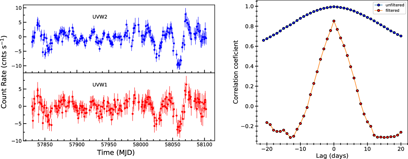
Figure 9. The light curves, filtered for the variations longer than 20 days, in UVW2 and UVW1 bands are shown in the top and bottom left panels, respectively. These filtered light curves are cross-correlated using ICCF method and resulting CCF distribution is shown in the right panel (in red circle) along with unfiltered CCF distribution (in blue circle).
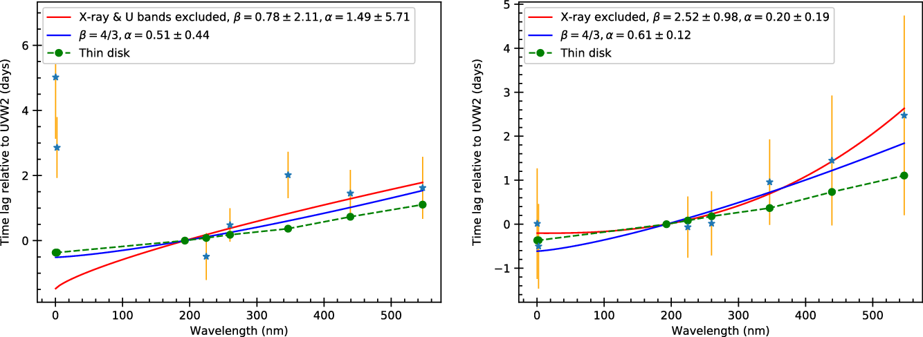
Figure 10. Wavelength-dependent lag spectrum modelling is shown for without filtering (left panel) and 18 days filtering (right panel) of light curves (i) with power law model
 $\tau\propto \lambda^{\beta}$
excluding X-ray data points (and U in the case of without filtering) and extrapolated down to X-ray (red solid line), (ii) with simple 4/3 power law (blue solid line), (iii) theoretically estimated time delay with respect to UVW2 band (green dashed line). Blue stars are the time lag values calculated from ICCF method.
$\tau\propto \lambda^{\beta}$
excluding X-ray data points (and U in the case of without filtering) and extrapolated down to X-ray (red solid line), (ii) with simple 4/3 power law (blue solid line), (iii) theoretically estimated time delay with respect to UVW2 band (green dashed line). Blue stars are the time lag values calculated from ICCF method.
Weak/moderate correlations between the X-rays and the UV/optical emission may be interpreted as due to the presence of fluctuations of different timescales. These fluctuations may be associated with the changes in the accretion rates according to the fluctuation propagation model proposed by Lyubarskii (Reference Lyubarskii1997). Typical timescale of variations expected for the UV/optical bands due to changes in the accretion rates are of the order of thousands or more years for AGNs like Mrk 509. These timescales are estimated for 1H 0419-577 by Pal et al. (Reference Pal, Dewangan, Kembhavi, Misra and Naik2018), which has a similar supermassive black hole mass (
 ${\sim}10^8\ {\rm M}_{\odot}$
).
${\sim}10^8\ {\rm M}_{\odot}$
).
The soft excess in AGNs is often explained by the relativistic blurred disk reflection model (Fabian et al. Reference Fabian, Iwasawa, Reynolds and Young2000; Fabian et al. Reference Fabian2009). According to this model, the accretion disk is illuminated by the X-ray power law continuum emission from the corona, producing a reflected spectrum. Reflection of continuum photons from the relativistically rotating inner disk gives rise to several smeared emission lines which look like a hump (an excess over the continuum emission) below
 $\sim$
2 keV. In the case of Mrk 509, however, the soft X-ray leads the hard X-ray (power law) emission as shown in Table 5, which is not compatible with the reflection model. Second, the low variability in hard X-ray and weak/moderate correlation between hard X-ray and UV/optical bands make it unlikely that the UV/optical emissions are driven by reflection.
$\sim$
2 keV. In the case of Mrk 509, however, the soft X-ray leads the hard X-ray (power law) emission as shown in Table 5, which is not compatible with the reflection model. Second, the low variability in hard X-ray and weak/moderate correlation between hard X-ray and UV/optical bands make it unlikely that the UV/optical emissions are driven by reflection.
4.2. Possibility of the X-ray reprocessing
X-ray reprocessing phenomenon is a process in which X-ray emission from the optically thin and hot plasma is reprocessed in the distant accretion disk to re-emit in the longer wavelengths (Krolik et al. Reference Krolik, Horne, Kallman, Malkan, Edelson and Kriss1991; Collier et al. Reference Collier, Horne, Wanders and Peterson1999). Confirmation of the X-ray reprocessing was first observed from UV/optical to infrared bands in a Seyfert 1 AGN NGC 2617 by Shappee et al. (Reference Shappee2014) and the lags at the longer wavelengths were found to be consistent with the predictions of the X-ray reprocessing in the standard accretion disk. In recent times, NGC 5548 has been the most studied AGN for the reverberation mapping of the accretion disk (Edelson et al. Reference Edelson2015; Fausnaugh et al. Reference Fausnaugh2016), and most of the studies hint towards a larger size of the accretion disk. Theoretically, in a geometrically thin and optically thick accretion disk, which is heated internally by viscous dissipation and externally by irradiation of the central UV/X-ray source, the temperature at a radius R from the centre is given by
 \begin{equation} T(R) = \Bigg( \frac{3GM \dot{M}}{8\pi \sigma R^3} + \frac{(1-A) L_x H}{4\pi \sigma R^3} \Bigg)^{1/4}, \end{equation}
where G, M,
 $\dot{M}$
,
$\dot{M}$
,
 $L_x$
, A, H, and
$L_x$
, A, H, and
 $\sigma$
are the gravitational constant, mass of the central SMBH, mass accretion rate, luminosity of the heating radiation, albedo of the accretion disk, height of the central heating source, and Stefan–Boltzmann constant, respectively (Cackett et al. Reference Cackett, Horne and Winkler2007). In this equation, the effects of inclination angle, relativistic effects in the inner part of the disk and the inner edge of the disk have been neglected. Following the steps given in Fausnaugh et al. (Reference Fausnaugh2016), the time delay
$\sigma$
are the gravitational constant, mass of the central SMBH, mass accretion rate, luminosity of the heating radiation, albedo of the accretion disk, height of the central heating source, and Stefan–Boltzmann constant, respectively (Cackett et al. Reference Cackett, Horne and Winkler2007). In this equation, the effects of inclination angle, relativistic effects in the inner part of the disk and the inner edge of the disk have been neglected. Following the steps given in Fausnaugh et al. (Reference Fausnaugh2016), the time delay
 $\tau$
relative to the reference time delay
$\tau$
relative to the reference time delay
 $\tau_0$
corresponding to reference wavelength
$\tau_0$
corresponding to reference wavelength
 $\lambda_0$
is given by
$\lambda_0$
is given by
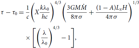 \begin{align} \tau-\tau_0 &= \frac{1}{c} \Bigg(X\frac{k\lambda_0}{hc} \Bigg)^{4/3} \Bigg( \frac{3GM\dot{M}}{8\pi\sigma} + \frac{(1-A) L_x H}{4\pi \sigma} \Bigg)^{1/3} \nonumber\\[2pt] &\quad \times \Bigg[\Bigg(\frac{\lambda}{\lambda_0}\Bigg)^{4/3}-1 \Bigg], \end{align}
where X is the multiplicative factor that takes into account systematic issues in the conversion of temperature T to wavelength
 $\lambda$
for a given R. The value of this factor is 4.87 when the temperature corresponding to the observed emission wavelength is given by Wein’s law and 2.49 when flux-weighted radius is used. In the flux-weighted case, the temperature profile of the accretion disk is described by the Shakura & Sunyaeav disk (
$\lambda$
for a given R. The value of this factor is 4.87 when the temperature corresponding to the observed emission wavelength is given by Wein’s law and 2.49 when flux-weighted radius is used. In the flux-weighted case, the temperature profile of the accretion disk is described by the Shakura & Sunyaeav disk (
 $T \propto R^{-3/4}$
). In both the cases, the disk is assumed to have a fixed aspect ratio all over. Equation (2) can be simplified by taking
$T \propto R^{-3/4}$
). In both the cases, the disk is assumed to have a fixed aspect ratio all over. Equation (2) can be simplified by taking
 $(1-A)L_xHR = \kappa GM\dot{M}/2R$
, where
$(1-A)L_xHR = \kappa GM\dot{M}/2R$
, where
 $\kappa$
is the local ratio of external to internal heating and independent of radius. Using luminosity of Mrk 509
$\kappa$
is the local ratio of external to internal heating and independent of radius. Using luminosity of Mrk 509
 $L_x$
as 1044 erg s–1 (Vasudevan & Fabian Reference Vasudevan and Fabian2009), coronal height H as 1.53
$L_x$
as 1044 erg s–1 (Vasudevan & Fabian Reference Vasudevan and Fabian2009), coronal height H as 1.53
 $r_g(=GM/c^2)$
(García et al. Reference García2019), and assuming albedo A equal to 0.2 (as used in several AGNs, e.g., McHardy et al. (Reference McHardy2014), Pal & Naik (Reference Pal and Naik2017)), the value of
$r_g(=GM/c^2)$
(García et al. Reference García2019), and assuming albedo A equal to 0.2 (as used in several AGNs, e.g., McHardy et al. (Reference McHardy2014), Pal & Naik (Reference Pal and Naik2017)), the value of
 $\kappa$
comes out as
$\kappa$
comes out as
 $\sim$
0.016. The smaller value of
$\sim$
0.016. The smaller value of
 $\kappa$
indicates that the contribution towards time delay due to external heating is insignificant (0.5%, estimated from Equation (2)) compared to viscous heating. Therefore, using Equation (3) from Edelson et al. (Reference Edelson2017), the time delays with respect to UVW2 (
$\kappa$
indicates that the contribution towards time delay due to external heating is insignificant (0.5%, estimated from Equation (2)) compared to viscous heating. Therefore, using Equation (3) from Edelson et al. (Reference Edelson2017), the time delays with respect to UVW2 (
 $\tau_0=0$
) band can be expressed as
$\tau_0=0$
) band can be expressed as
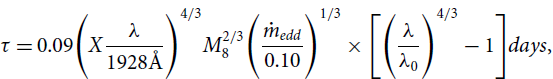 \begin{equation} \tau = 0.09 \Bigg(X \frac{\lambda}{1928\text{\rm{{\AA}}}} \Bigg)^{4/3} M_8^{2/3} \Bigg(\frac{\dot{m}_{edd}}{0.10} \Bigg)^{1/3}\times \Bigg[\Bigg(\frac{\lambda}{\lambda_0}\Bigg)^{4/3}-1 \Bigg] days,\end{equation}
where
 $M_8$
and
$M_8$
and
 $\dot{m}_{edd}$
are mass of the black hole in units of
$\dot{m}_{edd}$
are mass of the black hole in units of
 $10^8\,{\rm M}_{\odot}$
and the Eddington ratio (
$10^8\,{\rm M}_{\odot}$
and the Eddington ratio (
 $\dot{M}$
/
$\dot{M}$
/
 $\dot{M}_{edd}$
). This equation assumes negligible external heating by the UV/X-ray source compared to the internal viscous heating and radiation efficiency to be 0.1. We use the mass of the central SMBH of Mrk 509 to be
$\dot{M}_{edd}$
). This equation assumes negligible external heating by the UV/X-ray source compared to the internal viscous heating and radiation efficiency to be 0.1. We use the mass of the central SMBH of Mrk 509 to be
 $1.43\times10^8\,{\rm M}_\odot$
(Peterson et al. Reference Peterson2004),
$1.43\times10^8\,{\rm M}_\odot$
(Peterson et al. Reference Peterson2004),
 $\dot{m}_{edd}$
equal to 0.0951 (Vasudevan & Fabian Reference Vasudevan and Fabian2009), and X=2.49 for flux-weighted radius. Using the above values, the time delays with respect to the UVW2 band are estimated to be
$\dot{m}_{edd}$
equal to 0.0951 (Vasudevan & Fabian Reference Vasudevan and Fabian2009), and X=2.49 for flux-weighted radius. Using the above values, the time delays with respect to the UVW2 band are estimated to be
 $-0.367, -0.366, 0.083, 0.180, 0.367, 0.733$
, and
$-0.367, -0.366, 0.083, 0.180, 0.367, 0.733$
, and
 $1.106$
days for hard X-rays, soft X-rays, UVM2, UVW1, U, B, and V bands, respectively. In our analysis of unfiltered light curves of Mrk 509, we found delayed emission in hard X-ray, soft X-ray, UVW1, U, B, and V bands with respect to the emission in UVW2 band (Figure 10 & Table 5) while the delayed emission in the X-ray reprocessing is expected to be in the longer wavelength bands compared to the X-ray emission. Therefore, the observed positive lags in the X-ray bands are unexpected while considering the reprocessing scenario.
$1.106$
days for hard X-rays, soft X-rays, UVM2, UVW1, U, B, and V bands, respectively. In our analysis of unfiltered light curves of Mrk 509, we found delayed emission in hard X-ray, soft X-ray, UVW1, U, B, and V bands with respect to the emission in UVW2 band (Figure 10 & Table 5) while the delayed emission in the X-ray reprocessing is expected to be in the longer wavelength bands compared to the X-ray emission. Therefore, the observed positive lags in the X-ray bands are unexpected while considering the reprocessing scenario.
The estimated lags from the observed light curves may be affected due to the slow variations, for example, due to the fluctuations in the accretion flow. The reprocessed variable component in longer wavelength is diluted with the intrinsic emission due to the viscous heating in the accretion disk. Therefore, a possible origin of the variability in longer wavelengths could be a combination of two effects: reprocessing and propagating fluctuations. In the propagating fluctuation scenario, one expects the longer wavelength emission leading to the shorter wavelength emission. As the fluctuations propagate inwards through the accretion flow, it modulates the UV/optical and X-ray emission. Since the X-ray emitting region is very close to the central engine, it shows rapid fluctuations. These X-rays are again reprocessed to give longer wavelength emission. Therefore, there is always a tussle between the reprocessing and propagating fluctuations and the resultant time lag depends on the dominant process. Therefore, the geometry of the corona and the accretion disk are complex and both are not so simple as assumed in the lamp post model. After removing the slow variations of about 18 days, the trend in the estimated lags appear to be the same as the delayed hard X-ray emission as well as the optical emission (right panel of Figure 10).
4.3. Excess lags in U and X-ray band with respect to UVW2 band
The lags derived without removing the slow variations are shown in the left panel of Figure 10. This shows clear ‘excess’ lags in U as well as in X-ray bands with respect to the UVW2 band when fitted with the power law model
 $\tau \propto \lambda^{4/3}$
. Excess lag in U band was first reported by Korista & Goad (Reference Korista and Goad2001) in NGC 5548 and then in later studies (Edelson et al. Reference Edelson2015; Fausnaugh et al. Reference Fausnaugh2016; Pal & Naik Reference Pal and Naik2017; Naik et al. Reference Naik, Pal and Kumari2019) in different AGNs. Cackett et al. (Reference Cackett, Chiang, McHardy, Edelson, Goad, Horne and Korista2018) also found a strong excess in the Balmer jump region in NGC 4593. Korista & Goad (Reference Korista and Goad2001) predicted that there is a significant contribution of diffused emission from the BLR in UV bands. The wavelength-dependent lag across UV–optical energy range can imitate the lag spectrum originated as a result of X-ray reprocessing from the accretion disk. Similar results were found by Lawther et al. (Reference Lawther, Goad, Korista, Ulrich and Vestergaard2018) and they emphasised on the importance of diffuse continuum contribution while inferring the disk sizes on the basis of inter-band continuum delays. This feature has been observed in many Seyfert 1 galaxies, as shown by Edelson et al. (Reference Edelson2019) in four AGNs, including Mrk 509. Hernandez Santisteban et al. (Reference Hernandez Santisteban2020) modelled the lag spectrum of Fairall 9 by taking into account the contribution from the BLR (Figure 6 of their paper). Their modelling was based on the previous work on NGC 5548 by Korista & Goad (Reference Korista and Goad2019). On the basis of these results, it can be safely inferred that the BLR contribution in the inter-band lag spectra is unavoidable. As a result, the variability within the UV/optical can be inferred as the mixing of two effects: emission from standard Shakura–Sunyaev disk and diffused continuum emission from the BLR as discussed above.
$\tau \propto \lambda^{4/3}$
. Excess lag in U band was first reported by Korista & Goad (Reference Korista and Goad2001) in NGC 5548 and then in later studies (Edelson et al. Reference Edelson2015; Fausnaugh et al. Reference Fausnaugh2016; Pal & Naik Reference Pal and Naik2017; Naik et al. Reference Naik, Pal and Kumari2019) in different AGNs. Cackett et al. (Reference Cackett, Chiang, McHardy, Edelson, Goad, Horne and Korista2018) also found a strong excess in the Balmer jump region in NGC 4593. Korista & Goad (Reference Korista and Goad2001) predicted that there is a significant contribution of diffused emission from the BLR in UV bands. The wavelength-dependent lag across UV–optical energy range can imitate the lag spectrum originated as a result of X-ray reprocessing from the accretion disk. Similar results were found by Lawther et al. (Reference Lawther, Goad, Korista, Ulrich and Vestergaard2018) and they emphasised on the importance of diffuse continuum contribution while inferring the disk sizes on the basis of inter-band continuum delays. This feature has been observed in many Seyfert 1 galaxies, as shown by Edelson et al. (Reference Edelson2019) in four AGNs, including Mrk 509. Hernandez Santisteban et al. (Reference Hernandez Santisteban2020) modelled the lag spectrum of Fairall 9 by taking into account the contribution from the BLR (Figure 6 of their paper). Their modelling was based on the previous work on NGC 5548 by Korista & Goad (Reference Korista and Goad2019). On the basis of these results, it can be safely inferred that the BLR contribution in the inter-band lag spectra is unavoidable. As a result, the variability within the UV/optical can be inferred as the mixing of two effects: emission from standard Shakura–Sunyaev disk and diffused continuum emission from the BLR as discussed above.
In the simple picture of reprocessing model, X-ray emitting central corona illuminates and heats the accretion disk. The reprocessing model predicts that when
 $\tau \propto \lambda^{4/3}$
relation in UV/optical is extrapolated down to X-rays, it should fit the data well. But Figure 10, generated from unfiltered light curves for long-term variations, shows a huge discrepancy. Even after filtering, although excess lag was decreased significantly, the lags in hard X-rays still appear to be higher, which cannot be explained by a simple reprocessing model.
$\tau \propto \lambda^{4/3}$
relation in UV/optical is extrapolated down to X-rays, it should fit the data well. But Figure 10, generated from unfiltered light curves for long-term variations, shows a huge discrepancy. Even after filtering, although excess lag was decreased significantly, the lags in hard X-rays still appear to be higher, which cannot be explained by a simple reprocessing model.
4.4. Complex nature of the accretion disk
As the X-ray reprocessing phenomenon is unable to explain the observed lag spectrum successfully, this compels us to look for alternative models in explaining the observed correlated variability in the X-ray/UV/optical wave bands. One such model is given by Gardner & Done (Reference Gardner and Done2017) in which the excess lag of X-ray relative to UV band in NGC 5548 is explained. According to this model, the inner part of the accretion disk is called the Comptonization region, which is ‘puffed up’ and emits in EUV energy band. This region is heated by the hard X-rays coming from the central corona, producing heating waves which dissipate outwards. In response to these heating waves, the outer region of the disk expands and contracts and produces continuum lags. The model suggests the shorter wavelength lead the longer wavelength variations, which is not the case with Mrk 509 even after filtering. So this model does not explain the short-term variability seen in Mrk 509 for this particular duration of observations. Using XMM-Newton and Swift observations of Mrk 509 for a few days, Mehdipour et al. (Reference Mehdipour2011) inferred that the soft X-ray excess below 2 keV is produced by the Comptonization of the seed photons from the UV–optical disk into a warm and optically thick corona. This result seems to be consistent with the positive lag between UVW2 and X-rays found in our analysis.
The best-fitted value of power law normalisation
 $\alpha$
gives the size of the emitting region of reference wavelength, i.e., 1928Å (the central wavelength of the UVW2 band) if we assume the face-on standard disk. The size of the emitting region for the UVW2 emission can be estimated to be
$\alpha$
gives the size of the emitting region of reference wavelength, i.e., 1928Å (the central wavelength of the UVW2 band) if we assume the face-on standard disk. The size of the emitting region for the UVW2 emission can be estimated to be
 $0.61\times24\times60\times60\times 3\times10^{10}=1.58\times10^{15}$
cm which is equivalent to
$0.61\times24\times60\times60\times 3\times10^{10}=1.58\times10^{15}$
cm which is equivalent to
 $\sim$
80
$\sim$
80
 $R_{g}$
. Therefore, the size for the UVM2 and UVW1 emission would be similar as these bands show the time delays consistent with zero for the UVM2 and UVW1 bands with respect to the UVW2. In the case of variability, the fractional variability found in the UVW2 band is marginally higher than that seen in the UVM2 and UVW1 bands. The lags consistent with zero and similar amplitude of the variability in the UV bands suggest that the disk does not appear to have a smooth surface. Though the
$R_{g}$
. Therefore, the size for the UVM2 and UVW1 emission would be similar as these bands show the time delays consistent with zero for the UVM2 and UVW1 bands with respect to the UVW2. In the case of variability, the fractional variability found in the UVW2 band is marginally higher than that seen in the UVM2 and UVW1 bands. The lags consistent with zero and similar amplitude of the variability in the UV bands suggest that the disk does not appear to have a smooth surface. Though the
 $\beta=$
4/3 wavelength rule does not fit the lag spectrum well when the X-ray and U band lags are included; the spectrum is well described by this rule on excluding these excess lags. This implies that the reprocessed optical emission is likely caused by the UV emission with some delay. Excluding the X-ray lags, the fits corresponding to
$\beta=$
4/3 wavelength rule does not fit the lag spectrum well when the X-ray and U band lags are included; the spectrum is well described by this rule on excluding these excess lags. This implies that the reprocessed optical emission is likely caused by the UV emission with some delay. Excluding the X-ray lags, the fits corresponding to
 $\beta=2.52\pm0.98$
and the
$\beta=2.52\pm0.98$
and the
 $\beta=4/3$
values describe the lag spectrum well (right panel of Figure 10). These fits suggest that the UV emission is probably reprocessed in optical as well as in X-ray bands.
$\beta=4/3$
values describe the lag spectrum well (right panel of Figure 10). These fits suggest that the UV emission is probably reprocessed in optical as well as in X-ray bands.
The fitted
 $\beta$
values (
$\beta$
values (
 $0.78\pm2.11$
without X-ray and U;
$0.78\pm2.11$
without X-ray and U;
 $2.52\pm0.98$
after filtering) infer a complex structure of the accretion disk and even rules out a shell-like geometry (
$2.52\pm0.98$
after filtering) infer a complex structure of the accretion disk and even rules out a shell-like geometry (
 $\tau\propto\lambda^2$
) of emitting/reprocessing regions around the SMBH. Therefore, the actual disk is likely to be partly puffy, warped and inhomogeneous in nature and thus, the standard accretion theory seems not viable in the case of Mrk 509. The reason for getting lower lags after the process of filtering slow variations cannot be explained simply. In this process of removing of the slow components, it is not clear about the increased lags of V band, i.e.,
$\tau\propto\lambda^2$
) of emitting/reprocessing regions around the SMBH. Therefore, the actual disk is likely to be partly puffy, warped and inhomogeneous in nature and thus, the standard accretion theory seems not viable in the case of Mrk 509. The reason for getting lower lags after the process of filtering slow variations cannot be explained simply. In this process of removing of the slow components, it is not clear about the increased lags of V band, i.e.,
 ${\sim}1$
day for 10 days filtering and
${\sim}1$
day for 10 days filtering and
 ${\sim}3$
days for 20 days filtering. To answer the above questions and exploring such a complex nature of the accretion disk of Mrk 509 require a longer monitoring programme with a good cadence of observations compared to the available one.
${\sim}3$
days for 20 days filtering. To answer the above questions and exploring such a complex nature of the accretion disk of Mrk 509 require a longer monitoring programme with a good cadence of observations compared to the available one.
5. Summary
We analysed the X-ray and UV/optical data of Swift observatory spanning 2006–2019 to study the spectral and timing variability properties of Mrk 509. We applied different techniques to find out the correlation and time lags between different energy bands. We could see the correlation amongst all the energy bands by visual inspection. To quantify the correlation, we used count–count (or flux–flux) correlation with positive offset method. The time lags between various energy bands were estimated using ICCF and JAVELIN methods after filtering long variability components using the LOWESS method. The main results of our analysis are as follows:
-
1. Average spectrum over the entire duration shows that the soft X-ray excess is well described by two blackbody components with temperatures
 $kT_{\rm BB1}\sim120$
eV and
$kT_{\rm BB2}\sim460$
eV.
$kT_{\rm BB1}\sim120$
eV and
$kT_{\rm BB2}\sim460$
eV. -
2. We found a moderate/weak correlation between (i) the power law flux and BB flux and (ii) the blackbody temperature and BB flux.
-
3. Mrk 509 shows strong variability on short as well as long-term timescale (see variability amplitudes in Section 3.2.1) in all bands. Interestingly, the X-ray power law continuum shows smaller variability amplitude (
$\sim$
15%) compared to the soft X-ray and UV bands (
$\sim$
18–28%). -
4. The variability process in this AGN seems to be non-stationary (Figure 7). However, no spectral transition is observed over the years, as can be seen in Figure 3 where the power law photon index and blackbody temperature do not show any significant change.
-
5. The value of Pearson’s correlation coefficients for the UV/optical bands (
$\rho = 0.95{-}0.99$
with respect to the UVW2 bands and
$\rho = 0.40{-}0.53$
with respect to the hard X-ray) and corresponding p-values show that UV and optical bands are significantly correlated as compared to that of the X-ray emission and UV/optical bands. The hard X-ray emission is found to be well correlated with the soft X-ray emission (
$\rho$
= 0.82) while the hard X-ray and soft X-ray emission are correlated to the UVW2 emission with
$\rho$
values of 0.51 and 0.75, respectively. -
6. The positive offset resulting from the linear fit in the CP3O method with respect to UVW2 band suggests that the emission in UV and optical bands is less variable, while the negative offsets in the soft bands (soft X-ray/UV/optical) with respect to the hard X-ray power law continuum flux infer relatively more variabilities in the soft bands.
-
7. The time lags were estimated with respect to UVW2 energy band using ICCF and JAVELIN methods. The lags estimated from these two methods were comparable (within error). Before filtering the light curves for long-term variabilities, there was an excess lag in X-ray band and U band. After filtering for 18 days, the lag got reduced significantly.
-
8. The observed lags were found to increase with wavelength and were fitted with power law model by (i) keeping power law parameters (i.e.,
$\alpha$
and
$\beta$
) free with and without excluding hard and soft X-ray (ii) fixing
$\beta$
at
$4/3$
according to Shakura–Sunyaev accretion disk geometry. -
9. Our results favour the warm Comptonization region, located above the inner part of the accretion disk as the origin of the observed soft X-ray emission from Mrk 509. However, zero time lag and marginal variability difference between UV bands suggest that the UV emitting region in the disk is not smooth, instead a stratified region.


Acknowledgements
We thank the reviewer for his/her useful comments/suggestions which improved the paper significantly. The research work at PRL is funded by the Department of Space, Government of India. MP thanks the UGC, India for financial support through the DSKPDF fellowship grant no. BSR/2017-2018/PH/0111. For this research work, the software and online tools provided by the High Energy Astrophysics Science Archive Research Center (HEASARC) online service, maintained by the NASA/GFSC and the High Energy Astrophysics Division of the Smithsonian Astrophysical Observatory have been used. This work made use of data supplied by the UK Swift Science Data Centre at the University of Leicester.


