


1 INTRODUCTION
The planetary nebula (PN) PB 8 (PN G292.4+04.1) has been the subject of some recent studies (García-Rojas, Peña, & Peimbert Reference García-Rojas, Peña and Peimbert2009; Todt et al. Reference Todt, Peña, Hamann and Gräfener2010; Miller Bertolami et al. Reference Miller Bertolami, Althaus, Olano and Jiménez2011). The central star of PB 8 has been classified as [WC 5-6] by Acker & Neiner (Reference Acker and Neiner2003), as weak emission-line star type (wels; Tylenda, Acker, & Stenholm Reference Tylenda, Acker and Stenholm1993; Gesicki et al. Reference Gesicki, Zijlstra, Acker, Górny, Gozdziewski and Walsh2006), as [WC]-PG 1159 (Parthasarathy, Acker, & Stenholm Reference Parthasarathy, Acker and Stenholm1998), and finally as [WN/WC] hybrid by Todt et al. (Reference Todt, Peña, Hamann and Gräfener2010). Particularly, it is one of the rare stars, which has provoked a lot controversy about its evolutionary origin (Miller Bertolami et al. Reference Miller Bertolami, Althaus, Olano and Jiménez2011). A detailed abundance analysis of the nebula by García-Rojas et al. (Reference García-Rojas, Peña and Peimbert2009) showed abundance discrepancy factors (ADF ≡ ORL/CEL) of 2.57 for the O++ ion and 1.94 for the N++ ion, which are in the range of typical ADFs observed in PNe (ADFs ~ 1.6–3.2; see review by Liu Reference Liu, Barlow and Méndez2006). The nebular morphology was described as a round nebula with inner knots or filaments by Stanghellini, Corradi, & Schwarz (Reference Stanghellini, Corradi and Schwarz1993), and classified as elliptical by Gorny, Stasińska, & Tylenda (Reference Gorny, Stasińska and Tylenda1997). However, a narrow-band Hα+[N ii] image of PB 8 taken by Schwarz, Corradi, & Melnick (Reference Schwarz, Corradi and Melnick1992) shows a roughly spherical nebula with an angular diameter of about 7 arcsec (6.5 arcsec × 6.6 arcsec reported by Tylenda et al. Reference Tylenda, Siódmiak, Górny, Corradi and Schwarz2003), which is used throughout this paper.
The ionic abundances of heavy elements derived from optical recombination lines (ORLs) have been found to be systematically higher than those derived from collisionally excited lines (CELs) in many PNe (see e.g. Rola & Stasińska Reference Rola and Stasińska1994; Liu et al. Reference Liu, Storey, Barlow, Danziger, Cohen and Bryce2000, Reference Liu, Luo, Barlow, Danziger and Storey2001, Reference Liu, Barlow, Zhang, Bastin and Storey2006; Tsamis et al. Reference Tsamis, Barlow, Liu, Storey and Danziger2004; Tsamis, Walsh, Péquignot, Barlow, Danziger & Liu Reference Tsamis, Walsh, Péquignot, Barlow, Danziger and Liu2008; García-Rojas et al. Reference García-Rojas, Peña and Peimbert2009). To solve this problem, Liu et al. (Reference Liu, Storey, Barlow, Danziger, Cohen and Bryce2000) suggested a bi-abundance model in which the nebula contains two components of different abundances: cold hydrogen-deficient ‘metal-rich’ component and diffuse warm component of ‘normal’ abundances. The H-deficient inclusions embedded in the nebular gas of normal abundances can dominate the emissions of ORLs (Liu et al. Reference Liu, Storey, Barlow, Danziger, Cohen and Bryce2000, Reference Liu, Liu, Barlow and Luo2004). The bi-abundance photoionisation model of Abell 30 by Ercolano et al. (Reference Ercolano, Barlow, Storey, Liu, Rauch and Werner2003c) showed the possibility of such a scenario. More recently, the bi-abundance model by Yuan et al. (Reference Yuan, Liu, Péquignot, Rubin, Ercolano and Zhang2011) was able to predict the ORLs in NGC 6153. Previously, the analysis of the emission-line spectrum of NGC 6153 by Liu et al. (Reference Liu, Storey, Barlow, Danziger, Cohen and Bryce2000) pointed to a component of the ionised gas, cold and very metal-rich. The photoionisation modelling of NGC 1501 (Ercolano et al. Reference Ercolano, Wesson, Zhang, Barlow, De Marco, Rauch and Liu2004) and Abell 48 (Danehkar et al. Reference Danehkar, Todt, Ercolano and Kniazev2014) also suggested that they may contain some cold H-deficient structures.
The aim of this paper is to construct photoionisation models of PB 8, for which high-quality spectroscopy has become available (García-Rojas et al. Reference García-Rojas, Peña and Peimbert2009), constrained by an ionising source determined using the Potsdam Wolf-Rayet (PoWR) models for expanding atmospheres (Todt et al. Reference Todt, Peña, Hamann and Gräfener2010). To reproduce the observed ORLs, a bi-abundance model is used, which consists of a chemically homogeneous abundance distribution containing a small fraction of dense metal-rich structures. In addition, the dust properties are constrained using the Spitzer infrared (IR) continuum of the PN PB 8. The observations and modelling procedure are, respectively, described in Sections 2 and 3. In Section 4, we present our modelling results, while our conclusions are given in Section 5.
2 OBSERVATIONS
Deep optical long-slit spectra of the PN PB 8 were obtained at Las Campanas Observatory (PI: M. Peña), using the 6.5-m Magellan telescope and the double echelle Magellan Inamori Kyocera Echelle (MIKE) spectrograph on 2006 May 9 (García-Rojas et al. Reference García-Rojas, Peña and Peimbert2009). An observational journal is presented in Table 1. The standard grating settings used yield wavelength coverage from 3 350–5 050 Å in the blue and 4 950–9 400 Å in the red. The mean spectral resolution is 0.15 Å FWHM in the blue and 0.25 Å FWHM in the red. The MIKE observations were taken with three individual exposures of 300, 600, and 900 s using a slit of 1 × 5 arcsec2 and a position angle (PA) of 345° passing through the central star. To prevent contamination of the stellar continuum, an area of 0.9 × 1 arcsec2 on a bright knot located in the northern part of the slit was used to extract the nebular spectrum. However, there is no definite constraint on the location of the combined slit spectrum for the bright knot in the nebula, as the slit crossed over the nebula during the three different observations.Footnote 1 The top and bottom panels of Figure 1 show the blue and red spectra of PB 8 extracted from the 2D MIKE echellograms, normalised such that F(Hβ) = 100. As seen, several recombination lines from heavy element ions have been observed.

Figure 1. The observed optical spectrum of the PN PB 8 (García-Rojas et al. Reference García-Rojas, Peña and Peimbert2009), covering wavelengths of (top) 3 500–5 046 Å and (bottom) 5 047–8 451 Å, and normalised such that F(Hβ) = 100.
Table 1. Journal of the Observations for PB 8.

IR spectra of the PN PB 8 were taken on 2008 February 25 with the IR spectrograph on board the Spitzer Space Telescope (programme ID 40115, PI: Giovanni Fazio). The flux calibrated IR spectra used in this paper have been obtained from the Cornell Atlas of Spitzer/IR Spectrograph SourcesFootnote 2 (CASSIS; Lebouteiller et al. Reference Lebouteiller, Barry, Spoon, Bernard-Salas, Sloan, Houck and Weedman2011, Reference Lebouteiller, Barry, Goes, Sloan, Spoon, Weedman, Bernard-Salas and Houck2015). The Spitzer observations were taken with two low-resolution modules: Short–Low (SL) and Long–Low (LL). The SL spectrum was taken with an aperture size of 3.7 × 57 arcsec2 covering a wavelength coverage of 5.2–14.5 μm, whereas the LL spectrum has a wavelength coverage of 14.0–38.0 μm and an aperture size of 10.7 × 168 arcsec2. As the LL aperture is larger than the SL aperture, the LL module collects more flux than the SL, including the surrounding background contamination. This causes a jump at around 14 μm between the SL and the LL. To correct it, the LL spectrum was scaled to match the SL spectrum, so the combined Spitzer spectrum describes the thermal IR emission of the nebula with little background contribution. Table 2 lists the line fluxes measured from the Spitzer IR spectra (see Figure 5 for the Spitzer SL and LL combined spectrum). The intrinsic line fluxes presented in column 3 are on a scale where I(Hβ) = 100, and the dereddened flux I(Hβ) = 19.7 × 10⁻¹² erg cm−2 s−1 calculated using the total Hα flux (Frew, Bojičić, & Parker Reference Frew, Bojičić and Parker2013), E(B − V) = 0.41 and R V = 4 (Todt et al. Reference Todt, Peña, Hamann and Gräfener2010).
Table 2. IR line fluxes of the PN PB 8.
Note: Figure 5 shows the Spitzer spectrum (SL and LL combined).
Integral field unit (IFU) spectra were obtained at the Siding Spring Observatory on 2010 April 21 (programme ID 1100147, PI: Q.A. Parker), using the 2.3-m ANU telescope and the Wide Field Spectrograph (WiFeS; Dopita et al. Reference Dopita, Hart, McGregor, Oates, Bloxham and Jones2007, Reference Dopita2010). The settings used were the B7000/R7000 grating combination and the RT 560 dichroic, giving wavelength coverage from 4 415–5 589 Å in the blue and 5 222–7 070 Å in the red, and mean spectral resolution of 0.83 Å FWHM in the blue and 1.03 Å FWHM in the red (see the observational journal presented in Table 1). The WiFeS IFU rawdata were reduced using the iraf pipeline wifes, which consists of bias-reduction, sky-subtraction, flat-fielding, wavelength calibration using Cu–Ar arc exposures, spatial calibration using wire frames, differential atmospheric refraction correction, and flux calibration using spectrophotometric standard stars EG 274 and LTT 3864 (fully described in Danehkar, Parker, & Ercolano Reference Danehkar, Parker and Ercolano2013; Danehkar et al. Reference Danehkar, Todt, Ercolano and Kniazev2014).
Figure 2 shows the spatially resolved flux intensity and radial velocity maps of PB 8 extracted from the emission line [N ii] λ6 584 for spaxels across the WiFeS IFU field. The black/white contour lines depict the distribution of the emission of Hα obtained from the SuperCOSMOS Hα Sky Survey (SHS; Parker et al. Reference Parker2005), which can aid us in distinguishing the nebular borders. The emission line maps were obtained from solutions of the non-linear least-squares minimisation to a Gaussian curve function for each spaxel. The observed velocity V obs was transferred to the local standard of rest (LSR) radial velocity V LSR. The WiFeS IFU observations have recently been used for morpho-kinematic studies of PNe (Danehkar Reference Danehkar2015; Danehkar, Parker, & Steffen Reference Danehkar, Parker and Steffen2016). Considering the spatial resolution of the WiFeS (1 arcsec), this PN is very compact for detailed morpho-kinematic modelling. Following Danehkar & Parker (Reference Danehkar and Parker2015), the tenuous lobes of PB 8 extending from its compact core can be used to determine its spatial orientation. As seen in Figure 2, the orientation of its faint lobes onto the plane of the sky has a PA of 132° ± 8° relative to the north equatorial pole towards the east. Transferring into the Galactic coordinate system, its symmetric axis has a Galactic PA of 114.6° ± 8°, measured from the north Galactic pole towards the Galactic east, approximately aligned with the Galactic plane.
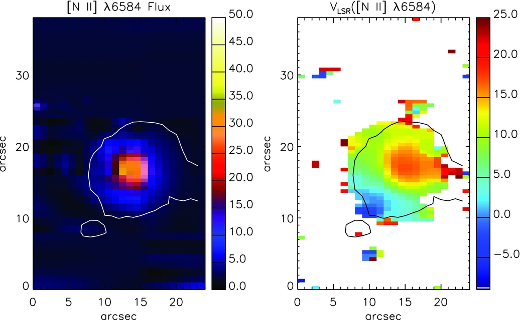
Figure 2. Maps of PB 8 in [N ii] λ6 584 from the IFU observation. From left to right: spatial distribution maps of flux intensity and LSR velocity. Flux unit is in 10−15 erg s−1 cm−2 spaxel−1, and velocity in km s−1. North is up and east is towards the left-hand side. The white/black contour lines show the distribution of the narrow-band emission of Hα in arbitrary unit obtained from the SHS (Parker et al. Reference Parker2005).
We obtained an expansion velocity of V exp = 20 ± 4 km s−1 from the [N ii] λ6 584 flux integrated across the whole nebula in the WiFeS field, which is in agreement with V exp = 19 km s−1 from [N ii] λ6 584 line derived by Todt et al. (Reference Todt, Peña, Hamann and Gräfener2010). Moreover, García-Rojas et al. (Reference García-Rojas, Peña and Peimbert2009) derived an expansion velocity of V exp = 14 ± 2 km s−1 from the [O iii] λ5007 line, which is associated with a different ionisation zone. García-Rojas et al. (Reference García-Rojas, Peña and Peimbert2009) obtained V sys = 1.4 km s−1 from [O iii] lines, in agreement with the value of V sys = 2.4 km s−1 given by Todt et al. (Reference Todt, Peña, Hamann and Gräfener2010).
3 PHOTOIONISATION MODELLING
The photoionisation modelling is performed using the mocassin code (version 2.02.70), described in detail by Ercolano et al. (Reference Ercolano, Barlow, Storey and Liu2003a) and Ercolano, Barlow, & Storey (Reference Ercolano, Barlow and Storey2005) in which the radiative transfer of the stellar and diffuse field is computed using a Monte Carlo (MC) method constructed in a cubical Cartesian grid, allowing completely arbitrary distribution of nebular density and chemical abundances. This code has already been used to study some chemical inhomogeneous models, namely the H-deficient knots of Abell 30 (Ercolano et al. Reference Ercolano, Barlow, Storey, Liu, Rauch and Werner2003c) and the super-metal-rich knots of NGC 6153 (Yuan et al. Reference Yuan, Liu, Péquignot, Rubin, Ercolano and Zhang2011). To solve the problem of ORL–CEL abundance discrepancies in those PNe, they used a metal-rich component, whose ratios of heavy elements with respect to H are higher than those of the normal component.
To investigate the abundance discrepancies between the ORLs and CELs, we have constructed different photoionisation models for PB 8. We run a set of model simulations, from which we finally selected three models, which best reproduced the observations. Our first model (MC1) consists of a chemically homogeneous abundance distribution. Our second model (MC2) is roughly similar, but it includes some dense metal-rich knots (cells) embedded in the density model of normal abundances (see Section 3.2). The final model (MC3) includes dust grains to match the Spitzer IR observation (see Section 3.4). The atomic data sets used for our models include energy levels, collision strengths, and transition probabilities from Version 7.0 of the chianti database (Landi et al. Reference Landi, Del Zanna, Young, Dere and Mason2012, and references therein), hydrogen and helium free-bound coefficients of Ercolano & Storey (Reference Ercolano and Storey2006), and opacities from Verner et al. (Reference Verner, Yakovlev, Band and Trzhaskovskaya1993) and Verner & Yakovlev (Reference Verner and Yakovlev1995).
The model parameters, as well as the physical properties for the models, are summarised in Table 3, and discussed in more detail in the following sections. The modelling procedure consists of an iterative process, involving the comparison of the predicted emission line fluxes with the values measured from the observations, and the ionisation and thermal structures with the values derived from the empirical analysis. The free parameters used in our models should be the nebular abundances, as the nebular density is adopted based on empirical results (García-Rojas et al. Reference García-Rojas, Peña and Peimbert2009), and the stellar parameters based on the model atmosphere study (Todt et al. Reference Todt, Peña, Hamann and Gräfener2010). However, it is impossible to isolate effects of any parameter from each other, as they are dependent on each other, so we cannot just modify the nebular abundances without slightly adjusting the density distribution and the distance. The nebular ionisation structure depends on the gas density and the stellar characteristics, so we fairly adjusted them to obtain the best-fitting models. We adopted the effective temperature of T eff = 52 kK, stellar luminosity of L ⋆ = 6000 L⊙, and non-local thermodynamic equilibrium (non-LTE) model atmosphere determined by Todt et al. (Reference Todt, Peña, Hamann and Gräfener2010). The optical depth for Lyman-continuum radiation of τ(Ly-c) = 0.63 estimated by Lenzuni, Natta, & Panagia (Reference Lenzuni, Natta and Panagia1989) indicated some ionising radiation fields may escape from the nebular shell, so it could be a matter-bounded PN. Therefore, we attempted to adjust distance and gas density to reproduce the nebular total Hβ intrinsic line flux. It is found that a model with an electron density of about 2550 ± 550 cm−3 empirically derived by García-Rojas et al. (Reference García-Rojas, Peña and Peimbert2009) can well reproduce the nebular Hβ intrinsic line flux at a distance of 4.9 kpc. We initially used the elemental abundances determined by García-Rojas et al. (Reference García-Rojas, Peña and Peimbert2009), but we adjusted them to match the observed nebular spectrum.
Table 3. Model parameters and physical properties for the final photoionisation models.
a The ORL empirical abundances were calculated from the ORLs over the total H+ emission flux, emitted from both the diffuse gas and metal-rich inclusion, so the empirical abundances of the ORLs cannot be the same as the model metal-rich component, but roughly similar to the mean total abundances of both the metal-rich and normal components.
3.1. The ionising spectrum
The H-deficient non-LTE model atmosphere (Todt et al. Reference Todt, Peña, Hamann and Gräfener2010), which was calculated using the PoWR models for expanding atmospheres (Gräfener, Koesterke, & Hamann Reference Gräfener, Koesterke and Hamann2002; Hamann & Gräfener Reference Hamann and Gräfener2004), was used as an ionising source in our photoionisation models. The PoWR models were constructed by solving the non-LTE radiative transfer equation of an expanding stellar atmosphere under the assumptions of spherical symmetry and chemical homogeneity. The PoWR model used was calculated for the stellar surface abundances H:He:C:N:O = 40:55:1.3:2:1.3 (by mass), the stellar temperature T eff = 52 kK, the stellar luminosity L ⋆ = 6000 L⊙, the transformed radius log R t = 1.43 R⊙ and the wind terminal velocity V ∞ = 1000 km s−1, which well matches the dereddened stellar spectra from FUSE, IUE, and MIKE, as well as 2MASS JHK bands (Todt et al. Reference Todt, Peña, Hamann and Gräfener2010). We see that the nebular [O iii] λ5 007 line flux relative to the Hβ flux is well reproduced with an effective temperature of T eff = 52 kK in our photoionisation models. The stellar luminosity of L ⋆ = 6000 L⊙ adopted by Todt et al. (Reference Todt, Peña, Hamann and Gräfener2010) is related to a remnant core with a typical mass of 0.6 M⊙ (e.g. Miller Bertolami & Althaus Reference Miller Bertolami and Althaus2007; Schönberner et al. Reference Schönberner, Jacob, Steffen, Perinotto, Corradi and Acker2005b). The distance was also varied in order to reproduce the nebular emission-line fluxes, under the constraints of our adopted stellar parameters and spherical density distribution. The best results for the photoionisation models were obtained at a distance of 4.9 kpc.
Figure 3 compares the non-LTE model atmosphere flux of PB 8 with a blackbody flux at the same temperature. At energies higher than 54 eV (He ii ground state), there is a significant difference between the non-LTE model atmosphere and blackbody flux. As discussed by Rauch (Reference Rauch2003), a blackbody is not an accurate representation of the ionising flux. The H-deficient non-LTE model atmosphere has a major departure from the solar model atmosphere at higher energies due to the small opacity from hydrogen. In our photoionisation models, we theretofore used an non-LTE model atmosphere as the ionising source to provide the best fit to the nebular spectrum. However, the difference may not be largely noticeable in our model as high-excitation lines (e.g. He ii) are not observed.
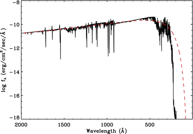
Figure 3. Non-LTE model atmosphere (solid line) calculated with T eff = 52 kK and chemical abundance ratio of H:He:C:N:O = 40:55:1.3:2:1.3 by mass (Todt et al. Reference Todt, Peña, Hamann and Gräfener2010), compared with a blackbody (dashed line) at the same temperature.
3.2. The density distribution
The initial nebular model to be run was the simplest possible density distribution, a homogeneous spherical geometry, to reproduce the CELs. The chemical abundances were taken to be homogeneous. A first attempt was made by using a homogeneous density distribution of 2 550 cm−3 with different inner and outer radii, deduced from the [O ii], [S ii], and [Cl iii] lines (García-Rojas et al. Reference García-Rojas, Peña and Peimbert2009). However, the uniform density distribution did not match the ionisation and thermal structures, so we examined different density distributions adopted based on radiation-hydrodynamics simulations (see e.g. Perinotto et al. Reference Perinotto, Schönberner, Steffen and Calonaci2004; Schönberner et al. Reference Schönberner, Jacob, Steffen, Perinotto, Corradi and Acker2005b; Schönberner, Jacob, & Steffen Reference Schönberner, Jacob and Steffen2005a) to make the best fit to the observed CELs, and also to constrain the shell thickness. Some radiation-hydrodynamics results depict a radial density profile having the form N H(r) = N 0[(r out/r)α], where r is the radial distance from the centre, α the radial density dependence, N 0 the characteristic density, and r out the outer radius. We finally adopted a density distribution with a powerlaw radial profile. Figure 4 illustrates the 3-D spherical density model constructed based on the radial density profile, and the ionising source is located in the corner. We chose the characteristic density of N 0 = 2600 cm−3 and the radial density dependence of α = −1. The outer radius of the sphere is equal to R out = 3.5 arcsec and the thickness is δR = 2.4 arcsec. We examined distances, with values within the range of distances 2.2 and 5.8 kpc (Phillips Reference Phillips2004, and references therein). The distance of D = 4.9 kpc found here, was chosen, because of the best predicted Hβ luminosity L(Hβ) = 4πD 2 I(Hβ), and it is within the range of distances 4.2 and 5.15 kpc estimated by Todt et al. (Reference Todt, Peña, Hamann and Gräfener2010). Taking the angular diameter of 7 arcsec, we derive an outer radios of R out = 2.6 × 1017 cm at the given distance of D = 4.9 kpc.
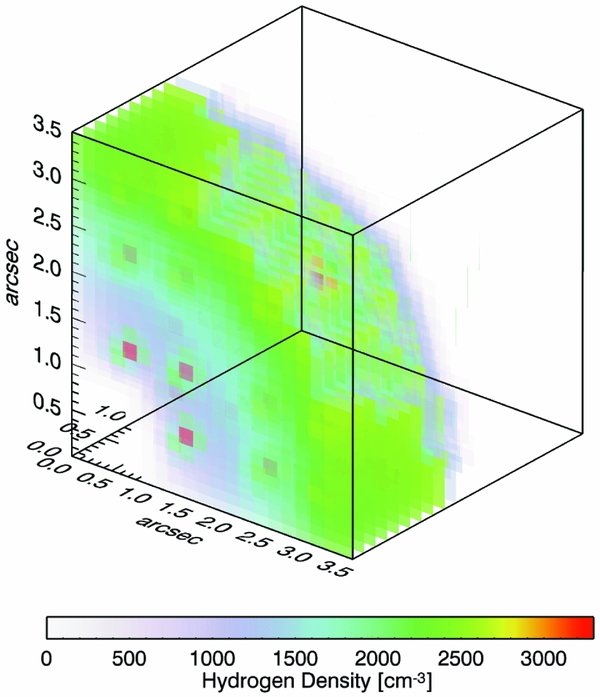
Figure 4. Spherical density distribution a power-law radial profile adopted for photoionisation models. The sphere has outer radius of 3.5 arcsec and thickness of 2.4 arcsec. The ionising source is placed in the corner (0, 0, 0). Metal-rich inclusions are shown as a darker knots with N H = 3300 cm−3 embedded in the density model of normal abundances. The units of the axes are arcsec.
A second attempt (MC2) was to reproduce the observed ORLs by introducing a fraction of metal-rich knots into the density distribution used by the first model. The abundance ratios of He, N, and O relative to H in the metal-rich component are higher than those in the normal component. Two different bi-abundance models suggested by Liu et al. (Reference Liu, Storey, Barlow, Danziger, Cohen and Bryce2000): one assumes that H-deficient component with a very high density (N e = 2 × 106 cm−3) and a moderate temperature (T e = 4700 K), which has been adopted in the bi-abundance photoionisation model of Abell 30 (Ercolano et al. Reference Ercolano, Barlow, Storey, Liu, Rauch and Werner2003c) and NGC 6153 (Yuan et al. Reference Yuan, Liu, Péquignot, Rubin, Ercolano and Zhang2011). However, H-deficient component in the second model introduced by Liu et al. (Reference Liu, Storey, Barlow, Danziger, Cohen and Bryce2000) has an eight times lower N e and a 20 times lower T e than the normal component. After exploring both the assumptions, we adopted a dense metal-rich component with the H number density of 3 300 cm−3, which is roughly 1.7 times higher than the mean density of the surrounding material.
In Figure 4, the 3-D spatial distribution of metal-rich knots (cells) are shown as a darker shade inside the density model of normal abundances. The gas-filling factor in the density model MC1 was kept at unity, while the inclusion of 33 metal-rich cells in the normal abundances nebula in the model MC2 (see Table 4) leads to gas-filling factors of 0.056 for the metal-rich component. It means that the dense metal-rich inclusions occupy 5.6% of the total gaseous volume of the nebula. Higher values of the gas-filling factor for the metal-rich component require lower values of the number density in order to reproduce the ORLs, but they may not provide the best match. We note that the filling factor parameter in mocassin is still set to 1.0, which can have a major role in emission-line calculations. For example, reducing the mocassin filling factor parameter from 1.0 to 0.5 decreases the nebular Hβ luminosity by a factor of 2 and increases the [O iii] λ5 007/Hβ flux ratio by 9%, so the nebula cannot be reproduced.
Table 4. Metal-rich component parameters in the model MC2.
For our bi-abundance model, we assume 33 metal-rich knots are uniformly distributed inside the diffuse warm nebula. However, Ercolano et al. (Reference Ercolano, Barlow, Storey, Liu, Rauch and Werner2003c) adopted a dense core surrounded by a less dense outer region in the bi-abundance model of Abell 30. Moreover, the metal-rich inclusions were distributed in the inner region of the diffuse warm nebula in the bi-abundance model of NGC 6153 (Yuan et al. Reference Yuan, Liu, Péquignot, Rubin, Ercolano and Zhang2011). Adopting the current knot density (3 300 cm−3) in PB 8, different distributions of metal-rich knots require totally different N/H and O/H abundance ratios and filling factors, which may not be in pressure equilibrium with their diffuse warm nebula. We note that ADFs of Abell 30 and NGC 6153 are very large, and are not similar to moderate ADFs of PB 8. Moreover, the effective temperatures of the central stars of Abell 30 and NGC 6153 are 130 000 and 90 000 K, respectively, which are hotter than T eff = 52 000 K in PB 8. This indicates that the central star of PB 8 is in an early stage of its evolutionary path towards becoming a white dwarf, and should be younger than the hot central stars of Abell 30 and NGC 6153.
The physical size of the metal-rich knots also play an important role in making an ionisation structure to reproduce the N ii and O ii ORLs. It is found that the physical size of (0.008)3 parsec3 (at D = 4.9 kpc) can well produce the observed ORLs. Reducing the physical size will lead to an increase in the number of knots, which also need different density or/and N/H and O/H abundance ratios to match the observation. Smaller sizes will contribute to higher ionisation and more thermal effects (see also Yuan et al. Reference Yuan, Liu, Péquignot, Rubin, Ercolano and Zhang2011), so we may not be able to reproduce electron temperatures estimated from the ORLs (see Section 4.2). A larger physical size will also decreases the number of knots, but it needs different density or/and different elemental abundances of N and O, which may not make metal-rich inclusions in pressure equilibrium with the surrounding gas.
3.3. The nebular elemental abundances
We used a homogeneous chemical abundance distribution for the model MC1 consisting of nine elements, including all the major contributors to the thermal balance of the nebula and those producing the density- and temperature-sensitive CELs. The abundances derived from the empirical analysis (García-Rojas et al. Reference García-Rojas, Peña and Peimbert2009) were chosen as starting values; these were iteratively modified to get a better fit to the CELs. The final abundance values are listed in Table 3, where they are given by number with respect to H.
A two-component elemental abundance distribution was used for the model MC2 that yields a better fit to the observed ORLs. The parameters of the metal-rich cells included in the bi-abundance model MC2 are summarised in Table 4. The metal-rich inclusions were constructed using 33 knots with the physical size of (0.35)3 arcsec3. As shown in Figure 4 (b), they are uniformly distributed inside the normal component model with the same geometry, but a filling factor of 0.056. The initial guesses at the elemental abundances of N and O in the metal-rich component were taken from the ORL empirical results; they were successively increased to fit the observed N ii and O ii ORLs. Table 3 lists the final elemental abundances (with respect to H) derived for both components, normal and metal-rich. The final model, which provided a better fit to most of the observed ORLs, has a total metal-rich mass of about 6.3% of the ionised mass of the entire nebula.
The O/H and N/H abundance ratios in the metal-rich component are about 1.0 and 1.7 dex larger than those in the normal component. The C/O abundance ratio in the metal-rich component less than unity is in disagreement with the theoretical predictions of born-again stellar models (Herwig Reference Herwig2001; Althaus et al. Reference Althaus, Serenelli, Panei, Córsico, García-Berro and Scóccola2005; Werner & Herwig Reference Werner and Herwig2006). As seen in Table 3, the ORL total abundances empirically derived were not similar to the elemental abundances chosen for the model metal-rich component. This is due to the fact that the ORL empirical abundances were derived from the ORLs, emitted mainly from metal-rich inclusion, over the H+ flux of the entire nebula, emitted from both the diffuse gas and metal-rich inclusion. Hence, the empirical abundances of the ORLs are roughly similar to the mean total abundances of both the metal-rich and normal components.
As seen in Table 3, the elemental abundance for neon does not show a large abundance discrepancy similar to what we see for oxygen and nitrogen, which is unlike to the bi-abundance models of Abell 30 (Ercolano et al. Reference Ercolano, Barlow, Storey, Liu, Rauch and Werner2003c) and NGC 6153 (Yuan et al. Reference Yuan, Liu, Péquignot, Rubin, Ercolano and Zhang2011). We note that the H-deficient knots of Abell 30 shows ADF(Ne++) values in the range of 400–1 000 (Wesson, Liu, & Barlow Reference Wesson, Liu and Barlow2003), and NGC 6153 has a ADF(Ne++) of about 60 (Liu et al. Reference Liu, Storey, Barlow, Danziger, Cohen and Bryce2000). Nevertheless, PB 8 has ADF(Ne++) = 1.48 (García-Rojas et al. Reference García-Rojas, Peña and Peimbert2009). To reproduce the spectrum of Abell 30, Ercolano et al. (Reference Ercolano, Barlow, Storey, Liu, Rauch and Werner2003c) also assumed a bi-abundance model, in which the metal-rich core has a density of about six times higher than the surrounding normal envelope. Thus, both Abell 30 and NGC 6153 have extremely large ADFs, which are dissimilar to PB 8. We should also include that the atomic data of the ORLs of Ne++ ion (Kisielius et al. Reference Kisielius, Storey, Davey and Neale1998) used by mocassin do not have any recombination coefficients for the Ne ii λ4391.94 and λ4409.30 lines, while García-Rojas et al. (Reference García-Rojas, Peña and Peimbert2009) employed different atomic data (Kisielius & Storey unpublished) to derive Ne++ ion abundance from for Ne ii ORLs.
It is worthwhile to mention that the AGB nucleosynthesis dramatically changes the composition of He, C, and N (Karakas & Lattanzio Reference Karakas and Lattanzio2003; Karakas et al. Reference Karakas, van Raai, Lugaro, Sterling and Dinerstein2009), but other elements such as Ne, S, Cl, and Ar are left untouched by the evolution and nucleosynthesis in low and intermediate-mass stars. In this typical PN with moderate ADFs, abundances of other elements heavier than oxygen such as neon in the metal-rich components seem to be the same as those in the normal component.
3.4. Dust modelling
PB 8 is known to be very dusty (e.g. Lenzuni et al. Reference Lenzuni, Natta and Panagia1989; Stasińska & Szczerba Reference Stasińska and Szczerba1999), which must influence the radiative processes in the nebula. Lenzuni et al. (Reference Lenzuni, Natta and Panagia1989) studied the IRAS measurements (25, 60, and 100 μm fluxes), and derived a dust temperature of T d = 85 ± 0.4 K, an optical depth of τ(Ly-c) = 0.63 and a dust-to-gas mass ratio of ρd/ρg = 0.0123 from a blackbody function fitted to the IRAS data. Similarly, Stasińska & Szczerba (Reference Stasińska and Szczerba1999) determined T d = 85 K, but ρd/ρg = 0.0096 from the broad band IRAS data. From the comparison of the mid-IR emission with a blackbody model of 150 K, Todt et al. (Reference Todt, Peña, Hamann and Gräfener2010) suggested that it possibly contains a warm dust with different dust compositions. We notice that the models MC1 and MC2 cannot provide thermal effects to account for the Spitzer IR continuum, so a dust component is necessary to reproduce the spectral energy distribution (SED) of the nebula observed in the IR range. The third model (MC3) presented here treats dust properties of PB 8 using the dust radiative transfer features included in the mocassin (Ercolano et al. Reference Ercolano, Barlow and Storey2005). Discrete grain sizes have been chosen based on the size range given by Mathis et al. (Reference Mathis, Rumpl and Nordsieck1977). The absence of the 9.7 μm amorphous silicate feature in the IR spectrum of PB 8 is commonly observed in O-rich circumstellar envelopes, which could imply this PN has a carbon-based dust. However, the strong features at 23.5, 27.5, and 33.8 μm are mostly attributed to crystalline silicates (Molster et al. Reference Molster, Waters, Tielens and Barlow2002). The features seen at 6.2, 7.7, 8.6, and 11.3 μm are related to polycyclic aromatic hydrocarbons (PAHs) (García-Lario et al. Reference García-Lario, Manchado, Ulla and Manteiga1999), together with broad features at 21 and 30 μm corresponding to a mixed chemistry having both O-rich and C-rich dust grains. The far-IR emission fluxes at 65 and 90 μm (Yamamura et al. Reference Yamamura, Makiuti, Ikeda, Fukuda, Oyabu, Koga and White2010) could be related to relatively warm forsterite grains, which emit at a longer wavelength. The 65 μm emission may be related to a crystalline water-ice structure, although its presence cannot be confirmed at the moment.
The thermal IR emission of PB 8 was modelled by adding a mixed dust chemistry to the pure-gas photoionisation model described in the previous sections. We explored a number of grain sizes and species, which could provide a best-fitting curve to the Spitzer IR continuum (see Figure 5). As seen, the model MC2 cannot produce the IR continuum, whereas the model MC3 fairly produces it. We tried to match the far-IR emission flux at 65 μm, while the 140 μm flux is extremely uncertain, F(140 μm) = 1.74 ± 3.33 Jy. The dust-to-gas mass ratio was varied until the best IR continuum flux was produced. Table 5 lists the dust parameters used for the final model of PB 8, the dust-to-gas ratio is given in Table 3. The geometry of the dust distribution is the same as the gas density distribution. The value of ρd/ρg = 0.01 found here is in agreement with Lenzuni et al. (Reference Lenzuni, Natta and Panagia1989). The final dust model incorporates two different grains, amorphous carbon, and crystalline silicate with optical constants taken from Hanner (Reference Hanner and Hanner1988) and Jaeger et al. (Reference Jaeger, Mutschke, Begemann, Dorschner and Henning1994), respectively. We also note that the nebular SED (shown in Figure 5), which is computed by mocassin, does not contain any contributions from the nebular emission line fluxes.
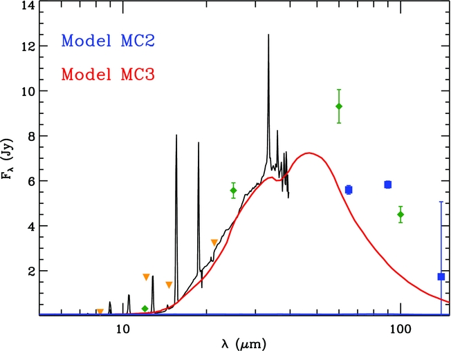
Figure 5. Observed Spitzer spectrum (black line) of PB 8 are compared with the continuum predicted by the model MC2 (blue line) and MC3 (red line). It also shows the photometric measurements for 12, 25, 60, and 100 μm (denoted by green diamonds) from IRAS (Helou & Walker Reference Helou and Walker1988), 8.3, 12.1, 14.7, and 21.34 μm (orange downward triangle) from MSX (Egan et al. Reference Egan2003), and the far-IR measurements (blue squares) F(65 μm) = 5.60 ± 0.19, F(90 μm) = 5.83 ± 0.16, and F(140 μm) = 1.74 ± 3.33 Jy from AKARI/FIS (Yamamura et al. Reference Yamamura, Makiuti, Ikeda, Fukuda, Oyabu, Koga and White2010). Note that the predicted nebular SED does not contain any nebular emission line fluxes.
Table 5. Input parameters for the dust model of PB 8.
For PB 8, Lenzuni et al. (Reference Lenzuni, Natta and Panagia1989) estimated a grain radius of 0.017 μm from the thermal balance equation under the assumption of the UV absorption efficiency Q UV = 1. Stasińska & Szczerba (Reference Stasińska and Szczerba1999) argued that the method of Lenzuni et al. underestimates the grain radius, and one cannot derive the grain size in such a way. Our photoionisation modelling implies that dust grains with a radius of 0.017 μm produce a very warm emission higher than T d = 85 K. The final dust model uses two discrete grain sizes, namely grain radii of 0.16 μm (warm) and 0.40 μm (cool), which can fairly reproduce the observed thermal IR SED with wavelengths less than 80 μm. Smaller grain sizes can produce hot emission that increases the continuum at shorter wavelengths (<10 μm), whereas larger grain sizes add cooler emission that may depict as a rise in the continuum at longer wavelengths (>80 μm). Although the current two grain sizes can well reproduce the Spitzer SED of PB 8, the solutions may not be unique. A dust model with more than two grain sizes may also be possible, but it needs more computational simulations to find the best-fit model. Moreover, inhomogeneous dust distribution and viewing angles (see Figure 2 in Ercolano et al. Reference Ercolano, Barlow and Storey2005) can also change the predicted SED. As there is no information on the inclination of dust grains and their geometry, so we assumed that they follow the gas density distribution.
There is a discrepancy in fluxes with wavelengths higher than 80 μm, which could be attributed to a possible inhomogeneous dust distribution. We note that the band measurements with wavelengths higher 100 μm could have high uncertainties, e.g. F(140 μm) = 1.74 ± 3.33 Jy. We also note a small discrepancy for fluxes with wavelengths less than 15 μm, which could be related to the difference between the SL aperture (3.7 × 57 arcsec2) and the LL aperture (10.7 × 168 arcsec2) used for the SL spectrum (5.2–14.5 μm) and the LL spectrum (14.0–38.0 μm), and uncertainties in scaling the LL spectrum (see Section 2). As both the LL and SL apertures covering some areas larger than the optical angular diameter of PB 8 (7 arcsec), they could also be contaminated by the ISM surrounding the nebula.
4 RESULTS
4.1. Comparison of the emission-line fluxes
Table 6 lists the observed and predicted nebular emission line fluxes. Column 4 presents the observed, dereddened intensities of PB 8 from García-Rojas et al. (Reference García-Rojas, Peña and Peimbert2009), relative to the intrinsic dereddened Hβ flux, on a scale where I(Hβ)=100. The ratios of predicted over observed values from the model MC1 are presented in Column 6. Columns 7–9 present the ratios of predicted over observed values for the normal component, the metal-rich component, and the entire nebula (normal+metal-rich) from the best-fitting model MC2. The same values obtained from the model MC3 are given in Columns 10–12. The majority of the CEL intensities predicted by model MC1 are in reasonable agreement with the observations. However, there are some large discrepancies between the prediction of model MC1 and the observations for ORLs. From the model MC2, it can be seen that the ORL discrepancy between model and observations can be explained by recombination processes of colder metal-rich inclusions embedded in the global H-rich environments.
Table 6. Comparison of predictions from the models and the observations. The observed, dereddened intensities are in units such that I(Hβ)=100. Columns (6)–(12) give the ratios of predicted over observed values in each case.
As seen in Table 6, the [N ii] λ6584 and [O iii] λ5007 line intensities predicted by the models MC1 and MC2 are in excellent agreement with the observations. As both the models MC2 and MC3 have exactly the same density distribution and chemical abundances, we can see how dust grains introduce a 10% increase in the [N ii] λ6584 line, which means that nitrogen abundance could be overestimated in some dusty nebulae. The H i line intensities as well as the majority of the He i line intensities are in reasonable agreement with the observations, discrepancies within 20%, apart from the He i λ3 889, λ5 875, and λ7 065 (around 30%). This could be due to high uncertainties of the recombination coefficients of the He i lines below 5 000 K (see Porter et al. Reference Porter, Ferland, Storey and Detisch2012, Reference Porter, Ferland, Storey and Detisch2013). The [O ii] λ7 319 and λ7 330 doublets are underestimated by around 50% in the model MC1. Recombination processes can largely contribute to the observed fluxes of these lines, which can be estimated by the empirical equation given by Liu et al. (Reference Liu, Storey, Barlow, Danziger, Cohen and Bryce2000) (see equation 2).
There are discrepancies between the predicted intensities of [S ii] and [S iii] lines and the observed values. While the intensities of the [S ii] lines are predicted to be about 10–20% lower than the observations, the intensity of the [S iii] λ6312 line is calculated to be almost twice more than the observed value. Adjusting the sulfur abundance cannot help reproduce [S iii] lines, so these discrepancies could be related to either the atomic data or the physical conditions. The predicted intensities of [S ii] lines were calculated using S+ collision strengths from Ramsbottom, Bell, & Stafford (Reference Ramsbottom, Bell and Stafford1996) incorporated into the chianti database (V 7.0), which is currently used in mocassin. Recently, new S+ collision strengths were calculated by Tayal & Zatsarinny (Reference Tayal and Zatsarinny2010), which ignored the effect of coupling to the continuum in their calculations, so their results were estimated to be accurate to about 30% or better. We note that the emissivities of [S ii] λλ6716,6731 lines calculated by the proequib IDL Library,Footnote 3 which includes an IDL implementation of the Fortran program equib (Howarth & Adams Reference Howarth and Adams1981; Howarth et al. Reference Howarth, Adams, Clegg, Ruffle, Liu, Pritchet and Ercolano2016), show that the collision strengths by Tayal & Zatsarinny (Reference Tayal and Zatsarinny2010) make them about 8% lower at the given physical conditions. The predicted [S iii] line intensities are perhaps much more uncertain, as there seem to be some errors in the atomic data, as mentioned by Grieve et al. (Reference Grieve, Ramsbottom, Hudson and Keenan2014). For example, the emissivity of [S iii] 18.68 μm line calculated using the collision strengths from Tayal & Gupta (Reference Tayal and Gupta1999) is about 40% higher than the calculation made with Hudson, Ramsbottom, & Scott (Reference Hudson, Ramsbottom and Scott2012) or Grieve et al. (Reference Grieve, Ramsbottom, Hudson and Keenan2014). This issue might be related to the long-standing problem of the sulfur anomaly in PNe (see reviews by Henry et al. Reference Henry, Speck, Karakas, Ferland and Maguire2012).
The predicted intensities of the [Ar iii] λλ7 136,7 751 lines are in agreement with the observations, discrepancies within 20%, however, the IR fine-structure [Ar iii] 8.99 μm line is predicted to be about 80% higher. We used Ar2 + collision strengths from Galavis, Mendoza, & Zeippen (Reference Galavis, Mendoza and Zeippen1995) used by the chianti database (V 7.0). There is another set for Ar2 + collision strengths (Munoz Burgos et al. Reference Munoz Burgos, Loch, Ballance and Boivin2009) whose predictions are significantly different and need to be examined carefully. We notice that the emissivities of [Ar iii] λλ7 136,7 751 lines predicted by proequib with the collision strengths from Munoz Burgos et al. (Reference Munoz Burgos, Loch, Ballance and Boivin2009) show a discrepancy of about 9% in comparison to those calculated with Galavis et al. (Reference Galavis, Mendoza and Zeippen1995), whereas there is a 30% difference in the [Ar iii] 8.99 μm emissivity calculated with the different atomic data.
The predicted [Ne ii] λ12.82 μm and [Ne iii] λλ3 869, 3 967 line intensities do not show high discrepancies (less than 20%), nevertheless, the calculated intensities of [Ne ii] λλ15.55,36.02 μm lines have discrepancies about 26 and 57%. The predicted [Cl iii] λλ5 518,5 538 lines are in agreement with the observations, discrepancies less than 25%.
Although the [O iii] λ4 363 auroral line is perfectly matched by the model MC3 and discrepancies remain less than 10% in the model MC2, there is a notable discrepancy in the [N ii] λ5 755 auroral line. This could be due to excitation by continuum fluorescence and/or recombination process. Bautista (Reference Bautista1999) found that the [N i] λλ5 198,5 200 lines are efficiently affected by fluorescence excitation in many objects, while [O i] lines were found to be sensitive to fluorescence in colder regions (⩽5000 K) or very high radiation fields. Nevertheless, this PN is not known to be surrounded by a photo-dissociation region (PDR) that is responsible for the fluorescence excitation. We notice that García-Rojas et al. (Reference García-Rojas, Peña and Peimbert2009) observed the brightest part of the nebula, and excluded the central star contamination and the surrounding potential PDR. Moreover, the absences of the [O i]λλ6 300,6 364 lines emitted by neutral O0 ion and the [N i]λλ5 198,5 200 lines emitted by neutral N0 ion in the spectrum presented by García-Rojas et al. (Reference García-Rojas, Peña and Peimbert2009) exclude any possibilities of the fluorescence contamination. Hence, there is no strong evidence for any possible fluorescence contributions to the observed fluxes. Alternatively, the recombination contribution to [N ii] auroral lines may have some implications, which can be estimated for low-density uniform nebular media (see, e.g. Liu et al. Reference Liu, Storey, Barlow, Danziger, Cohen and Bryce2000).
The recombination contribution to the [N ii] λ5 755 line and the [O ii] λλ7 320,7 330 doublet can be estimated as follows (Liu et al. Reference Liu, Storey, Barlow, Danziger, Cohen and Bryce2000):
 $$\begin{equation}
\frac{I_{\rm R}(\lambda 5\,755)}{I({\rm H}\beta )} = 3.19 \,\, {t^{0.30}} \, \bigg ( \frac{\rm N^{2+}}{\rm H^{+}} \bigg )_{\rm ORLs}, \\
\end{equation}$$
$$\begin{equation}
\frac{I_{\rm R}(\lambda 5\,755)}{I({\rm H}\beta )} = 3.19 \,\, {t^{0.30}} \, \bigg ( \frac{\rm N^{2+}}{\rm H^{+}} \bigg )_{\rm ORLs}, \\
\end{equation}$$
 $$\begin{equation}
\frac{I_{\rm R}(\lambda 7\,320+\lambda 7\,330)}{I({\rm H}\beta )} = 9.36 \,\, {t^{0.44}} \, \bigg ( \frac{\rm O^{2+}}{\rm H^{+}} \bigg )_{\rm ORLs},
\end{equation}$$
$$\begin{equation}
\frac{I_{\rm R}(\lambda 7\,320+\lambda 7\,330)}{I({\rm H}\beta )} = 9.36 \,\, {t^{0.44}} \, \bigg ( \frac{\rm O^{2+}}{\rm H^{+}} \bigg )_{\rm ORLs},
\end{equation}$$
Table 7. Mean electron temperatures (K) weighted by ionic species for the entire nebula. For each element, the first row is for MC1 and the second row is for MC2.
Table 8. Mean electron temperatures (K) weighted by ionic species for the nebula obtained from the photoionisation model MC3. For each element, the first row is for the normal component, the second row is for the H-poor component, and the third row is for the entire nebula.
Table 9. Fractional ionic abundances obtained from the photoionisation models. For each element, the first row is for MC1, the second row is for MC2, and the third row is for MC3.
Table 10. Fractional ionic abundances obtained from the photoionisation model MC2. For each element, the first row is for the normal component and the second row is for the H-poor component.

The intensities of the ORLs predicted by the model MC2 and MC3, both bi-abundance models, can be compared to the observed values in Table 6. Figure 6 compares the predicted over observed flux ratio for the model MC3, and shows the relative contributions of the normal and the metal-rich components to each emission-line flux. The agreement between the ORL intensities predicted by the two latter models and the observations is better than those derived from the first model (MC1). The majority of the O ii lines with strong intensities are in reasonable agreement with the observations, with discrepancies below 40%, except for λ4649.13, λ3749.48, λ4075.86, λ4132.80, and λ4153.30. The well-measured N ii λ5666.64, λ5676.02, and λ5679.56 lines are in good agreement with the observations, and discrepancies are less than 30%. There are some discrepancies in some O ii ORLs (e.g. λ4416.97, λ4121.46, and λ4906.81) and N ii ORLs (e.g. λ4601.48, λ4613.87, and λ5931.78), which have weak intensities and higher uncertainties (20–30%). However, as seen in Figure 6, the model MC3 has significant improvements in predicting the O ii and N ii lines having intensities stronger than other ORLs. Particularly, the bi-abundance models MC2 and MC3 provide better predictions for the O ii ORLs from the V1 multiplet and the N ii ORLs from the V3 multiplet, which have the reliable atomic data. Comparing Figure 6 with Figure 15 in Yuan et al. (Reference Yuan, Liu, Péquignot, Rubin, Ercolano and Zhang2011) demonstrates that our bi-abundance models of PB 8, similar to the photoionisation model of NGC 6153, better predict the observed intensities of the N ii and O ii ORLs. The models also reproduce the C ii ORLs with discrepancies about 10%, except the C ii λ6 578 line. The C ii λ4267.2 line is stronger than the other C ii lines, and it is not blended with any nearby O ii ORLs. The C ii λ6 578 line may be blended with nearby lines, so its measured line strength may be uncertainty.

Figure 6. The predicted over observed flux ratio for the bi-abundance model MC3. The relative contributions of the normal and the metal-rich components to each line flux are shown by black and grey parts, respectively.
4.2. Thermal structure
Table 7 lists the mean electron temperatures of the entire nebula in the models MC1 and MC2 weighted by ionic species, from the neutral (i) to the highly ionised ions (vii). The definition for the weighted-mean temperatures was given in Ercolano et al. (Reference Ercolano, Morisset, Barlow, Storey and Liu2003b). The value of T e(N ii) = 7746 K predicted by the model MC1 is about 1 150 K lower than the value of T e(N ii) = 8900 ± 500 K empirically derived from CELs by García-Rojas et al. (Reference García-Rojas, Peña and Peimbert2009). This could be due to recombination contributions to the auroral line. The recombination contribution estimated [using equation 1 in Liu et al. (Reference Liu, Storey, Barlow, Danziger, Cohen and Bryce2000)] about 12% in the model MC1 is much lower to explain the measured intensity of the [N ii] λ5 755 line. However, the model MC2 predicts the [N ii] λ5 755 line to be 40% higher than the value derived from the model MC1 (see recombination contribution estimated by equation (1) in Table 6). We also notice that the [N ii] temperature is roughly equal to the [O iii] temperature in low excitation PNe (Kingsburgh & Barlow Reference Kingsburgh and Barlow1994), so the empirical value of the [N ii] electron temperature derived by García-Rojas et al. (Reference García-Rojas, Peña and Peimbert2009) is difficult to be explained. The temperature T e(O ii) = 7746 K predicted by the model MC1 is about 670 k higher than T e(O ii) = 7050 ± 400 K empirically derived by García-Rojas et al. (Reference García-Rojas, Peña and Peimbert2009), while T e(O ii) = 6692 K predicted by the model MC2 is about 360 k lower than the empirical value. Moreover, the temperature of [O iii] calculated from the model MC1, T e(O iii) = 7613 K, is about 710 K higher the empirical result of T e(O iii) = 6900 ± 150 K, whereas T e(O iii) = 6568 K predicted by the model MC2 is about 330 K lower the empirical value.
Table 8 presents the electron temperatures of the different components of the model MC3 weighted by ionic abundances, as well as the mean temperatures of the entire nebula. The first entries for each element are for the normal abundance plasma, the second entries are for the metal-rich inclusion, and the third entries are for the entire nebula (including both the normal and the H-poor components). It can be seen that the temperatures weighted by ionic abundances in the two different components of the nebula are very different. The electron temperatures separately weighted by the ionic species of the metal-rich inclusions were much lower than those from the normal part. The temperature of T e(N ii) = 7315 K predicted by the normal component of the model MC3 is about 1 590 K lower than the value empirically derived. However, T e(O ii) = 7319 K and T e(O iii) = 7064 K obtained by the normal component of the model MC3 are in reasonable agreement with the values empirically derived by García-Rojas et al. (Reference García-Rojas, Peña and Peimbert2009). We see that T e(He i) = 4309 K weighted by the metal-rich component of the model MC3 is lower than the empirical value, T e(He i) = 6250 ± 150 K (García-Rojas et al. Reference García-Rojas, Peña and Peimbert2009), whereas T e(He i) = 6640 K weighted by the whole nebula is about 390 K higher the empirical value Moreover, T e(H i) = 4309 K weighted by the metal-rich component and T e(H i) = 6640 K weighted by the whole nebula are reasonably in the range of T e(H i) = 5100 + 1300 − 900 K empirically derived from the Balmer Jump to H11 flux ratio (García-Rojas et al. Reference García-Rojas, Peña and Peimbert2009). We take no account for the interaction between the two components, namely normal and metal-rich, which could also lead to a temperature variation. Note that the radiative transfer in a neutral region is not currently supported by MOCASSIN, so the code only estimates temperatures that likely correspond to a potential narrow transition region between ionised and neutral regions for a radiation-bounded object. Neutral elements in this PN are negligible (see Table 9), so the temperatures of the neutral species listed in Table 8 do not have any significant physical meaning. We also see that the two components have a local thermal pressure ratio of P(metal-rich)/P(normal) ~ 1.1, which means each metal-rich cell is in pressure equilibrium with its surrounding normal gas. The higher thermal pressure forces the dense, metal-rich knots to expand and reduce their density and temperature during the evolution phase of the nebula.
4.3. Fractional ionic abundances
Table 9 lists the volume-averaged fractional ionic abundances from the neutral (i) to the highly ionised ions (vii) calculated from the three models, where, the first entries for each element are for the chemically homogeneous model MC1, the second entries are for the bi-abundance model MC2, and the third entries are the dusty bi-abundance model MC3. The definition for the volume-averaged fractional ionic abundances was given in Ercolano et al. (Reference Ercolano, Morisset, Barlow, Storey and Liu2003b). We see that both hydrogen and helium are fully singly ionised, i.e. neutrals are almost 0% in the three models. It can be seen that the ionisation structure in MC2 is in reasonable agreement with MC1. The elemental oxygen largely exists as O2 + with 91% and then O+ with 9% in the model MC1, whereas O2 + is about 87% and then O+ is about 13% in the model MC2. Moreover, the elemental nitrogen largely exists as N2 + with 93% and then N+ with 7% in the model MC1, whereas N2 + is about 91% and then N+ is about 9% in the model MC2. The O+/O ratio is about 1.4–1.6 times higher than the N+/N ratio, which is in disagreement with the general assumption of N/N+=O/O+ in the ionisation correction factor (icf) method by Kingsburgh & Barlow (Reference Kingsburgh and Barlow1994), introducing errors to empirically derived elemental abundances. Our (N+/N)/(O+/O) ratio is in agreement with the value of 0.6–0.7 predicted by the photoionisation model of NGC 7009 implemented using mocassin (Gonçalves et al. Reference Gonçalves, Ercolano, Carnero, Mampaso and Corradi2006). While the assumption N/N+=O/O+ overestimates the N/H elemental abundance, the new icf(N/O) calculated using 1-D photoionisation modelling provides a better agreement (Delgado-Inglada, Morisset, & Stasińska Reference Delgado-Inglada, Morisset and Stasińska2014). Moreover, the O2 +/O ratio is about 1.1–1.2 higher than the Ne2 +/Ne ratio, in reasonable agreement with the assumption for the icf(Ne). The ionic fraction of S, Cl, and Ar predicted by MC2 are approximately about the values calculated by MC1. The small discrepancies in fractional ionic abundances between MC1 and MC2 can be explained by a small fraction of the metal-rich structures included in MC2.
The volume-averaged fractional ionic abundances calculated from the model MC2 are listed in Table 10, the upper entries for each element in the table are for the normal component and the lower entries are for the metal-rich component of the nebula. It can be seen that the model MC2 predict different ionic fractions of O+ for the two components of the nebula, whereas roughly the same value for N+. The O+/O ratios in the metal-rich component are about 20% higher than those in the normal component. This means that that the icf from CELs are not entirely accurate for deriving the elemental abundances from ORLs as adopted by some authors (see, e.g. Wang & Liu Reference Wang and Liu2007).
5 CONCLUSIONS
Three photoionisation models have been constructed for the PN PB 8, a chemically homogeneous model, a bi-abundance model and a dusty bi-abundance model. Our intention was to construct a model that well reproduce the observed emission-lines and thermal structure determined from the plasma diagnostics. A power-law radial density profile was adopted for the spherical nebula distribution based on the radiation-hydrodynamics simulations. The density model parameters were adjusted to reproduce the total Hβ intrinsic line flux of the nebula, and the mean electron density empirically derived from the CELs (García-Rojas et al. Reference García-Rojas, Peña and Peimbert2009). We have used the non-LTE model atmosphere derived by Todt et al. (Reference Todt, Peña, Hamann and Gräfener2010) for temperature T eff = 52 kK and luminosity L ⋆ = 6000 L⊙. This ionising source well reproduced the nebular observed Hβ absolute flux, as well as the [O iii] λ5 007 line flux, at the distance of 4.9 kpc.
Our initial model reproduces the majority of CELs and the thermal structure, but large discrepancies exist in the observed ORLs from heavy element ions. It is found that a chemically homogeneous model cannot consistently explain the ORLs observed in the nebular spectrum. We therefore intended to address the cause of the heavily underestimated ORLs. Following the hypothesis of the bi-abundance model by Liu et al. (Reference Liu, Storey, Barlow, Danziger, Cohen and Bryce2000), a small fraction of metal-rich inclusions was introduced into the second model. The heavy element ORLs are mostly emitted from the metal-rich structures embedded in the dominant diffuse warm plasma of normal abundances. The agreement between the ORL intensities predicted by the model MC2 and the observations is better than the first model (MC1). The metal-rich inclusions occupying 5.6% of the total volume of the nebula, and are about 1.7 times cooler and denser than the normal composition nebula. The O/H and N/H abundance ratios in the metal-rich inclusions are ~ 1.0 and 1.7 dex larger than the diffuse warm nebula, respectively. The mean electron temperatures predicted by MC2 are lower than those from MC1, which is because of the cooling effects of the metal-rich inclusions. The results indicate that a bi-abundance model can naturally explain the heavily underestimated ORLs in the chemically homogeneous model. Therefore, the metal-rich inclusions may solve the problem of ORL/CEL abundance discrepancies. However, the model MC2 cannot explain the thermal SED of the nebula observed with the Spitzer spectrograph. In our final model, we have incorporated a dual dust chemistry consisting of two different grains, amorphous carbon and crystalline silicate, and discrete grain radii. It is found that a dust-to-gas ratio of 0.01 by mass for the whole nebula can roughly reproduce the observed IR continuum.
The PN PB 8 shows moderate ADFs (~ 1.9–2.6; García-Rojas et al. Reference García-Rojas, Peña and Peimbert2009), which are typical of most PNe (see, e.g. Liu Reference Liu, Barlow and Méndez2006). Previously, the bi-abundance model were only examined in two PNe with extremely large ADFs: Abell 30 (Ercolano et al. Reference Ercolano, Barlow, Storey, Liu, Rauch and Werner2003c) and NGC 6153 (Yuan et al. Reference Yuan, Liu, Péquignot, Rubin, Ercolano and Zhang2011). In Abell 30, Ercolano et al. (Reference Ercolano, Barlow, Storey, Liu, Rauch and Werner2003c) used a metal-rich core whose density is about six times larger than the surrounding nebula. In NGC 6153, Yuan et al. (Reference Yuan, Liu, Péquignot, Rubin, Ercolano and Zhang2011) used super-metal-rich knots distributed in the inner region of the nebula. In the present study, we adopted a bi-abundance model whose metal-rich knots are homogeneously distributed inside the diffuse warm nebula, and are associated with a gas-filling factors of 0.056. To reproduce the spectrum of PB 8, it is not require to have extremely dense and super-metal-rich knots, since the ORLs do not correspond to very cold temperatures and extremely large ADFs such as Abell 30 and NGC 6153. We should mention that the stellar temperatures of Abell 30 (T eff = 130 kK) and NGC 6153 (T eff = 90 kK) are higher than that of PB 8 (T eff = 52 kK), so the central star of PB 8 is likely in an early stage of its stellar evolution towards a white dwarf in comparison with Abell 30 and NGC 6153. Accordingly, the PN PB 8 could be younger and less evolved than the PNe Abell 30 and NGC 6153. More recently, it has been found that PNe with ADFs larger than 10 mostly contain close-binary central stars (Corradi et al. Reference Corradi, García-Rojas, Jones and Rodríguez-Gil2015; Jones et al. Reference Jones, Wesson, García-Rojas, Corradi and Boffin2016; Wesson et al. Reference Wesson, Jones, García-Rojas, Corradi, Boffin, Liu, Stanghellini and Karakas2014). Currently, there is no evidence for a close-binary central star in PB 8.
Our analysis showed that the bi-abundance hypothesis, which was previously tested in a few PNe with very large abundance discrepancies, could also be used to explain moderate discrepancies between ORL and CEL abundances in most of typical PNe (ADFs ~ 1.6–3.2; Liu Reference Liu, Barlow and Méndez2006). It is unclear whether there is any link between the supposed metal-rich inclusions within the nebula and hydrogen-deficient stars. It has been suggested that a (very-) late thermal pulse is responsible for the formation of H-deficient central stars of planetary nebulae (see, e.g. Blöcker Reference Blöcker2001; Herwig Reference Herwig2001; Werner Reference Werner2001; Werner & Herwig Reference Werner and Herwig2006). Thermal pulses normally occur during the AGB phase, when the helium-burning shell becomes thermally unstable. The (very-) late thermal pulse occurs when the star moves from the AGB phase towards the white dwarf. It returns the star to the AGB phase and makes a H-deficient stellar surface, so called born-again scenario. However, the metal-rich component with C/O <1 predicted by our photoionisation models is in disagreement with the products of a born-again event (Herwig Reference Herwig2001; Althaus et al. Reference Althaus, Serenelli, Panei, Córsico, García-Berro and Scóccola2005; Werner & Herwig Reference Werner and Herwig2006).
It is also possible that the metal-rich inclusions were introduced by other mechanism such as the evaporation and destruction of planets by stars (Liu Reference Liu, Kwok, Dopita and Sutherland2003). Recently, Nicholls, Dopita, & Sutherland (Reference Nicholls, Dopita and Sutherland2012) and Nicholls et al. (Reference Nicholls, Dopita, Sutherland, Kewley and Palay2013) proposed that a non-Maxwellian distribution of electron energies could explain the abundance discrepancy. However, Zhang, Liu, & Zhang (Reference Zhang, Liu and Zhang2014) found that both the scenarios, bi-abundance models and non-Maxwellian distributed electrons, are adequately consistent with observations of four PNe with very large ADFs. It is unclear whether chemically inhomogeneous plasmas introduce non-Maxwell–Boltzmann equilibrium electrons to the nebula. Alternatively, the binarity characteristics such as the orbital separation and companion masses may have a leading role in forming different abundance discrepancies in those PNe with binary central stars (see, e.g. Herwig Reference Herwig2001; Althaus et al. Reference Althaus, Serenelli, Panei, Córsico, García-Berro and Scóccola2005). Further studies are necessary to trace the origin of possible metal-rich knots within the nebula and the cause of various abundance discrepancies in PNe.
ACKNOWLEDGEMENTS
AD is supported by a Macquarie University Research Excellence Scholarship (MQRES) and a Sigma Xi Grants-in-Aid of Research (GIAR). AD thanks the anonymous referee for helpful suggestion and comments that improved the paper, Helge Todt for providing the PoWR models for expanding atmospheres and valuable comments, Jorge García-Rojas and Miriam Peña for providing the Magellan Telescope data and helpful comments, Ralf Jacob for sharing results from radiation-hydrodynamics simulations and valuable suggestions, Christophe Morisset for illuminating discussions and corrections, Quentin A. Parker for providing the 2010 ANU 2.3-m data, David J. Frew for helping with the ANU observing proposal, Kyle DePew for carrying out the 2010 ANU observing run, and Roger Wesson for sharing the program equib (originally written by I. D. Howarth and S. Adams at UCL). The computations in this paper were run on the NCI National Facility in Canberra, Australia, which is supported by the Australian Commonwealth Government, the swinSTAR supercomputer at Swinburne University of Technology, and the Odyssey cluster supported by the FAS Division of Science, Research Computing Group at Harvard University.


