


1. Introduction
The Parkes 64-m diameter telescope remains a cutting-edge instrument because of the numerous upgrades that have occurred since it was built in 1961 (see, e.g., Edwards Reference Edwards2012). Astronomical requirements have continued to push for receivers that have wider fields of view and/or wider observing bandwidths. Multibeam receivers, such as the 13-beam 20-cm receiver (Staveley-Smith et al. Reference Staveley-Smith1996) and the 7-beam ‘methanol’ receiver (Green et al. Reference Green2009), have successfully carried out large-scale survey observations. More recently, an Australian Square Kilometer Array Pathfinder (ASKAP) phased array feed has been productively trialled at Parkes (Deng et al. Reference Deng2017; Reynolds et al. Reference Reynolds, Staveley-Smith, Rhee, Westmeier, Chippendale, Deng, Ekers and Kramer2017).
A dual-band receiver has been the primary receiver system for the Parkes Pulsar Timing Array (PPTA) project (Manchester et al. Reference Manchester2013), which carries out high-precision timing observations of pulsars in the hunt for ultra-low-frequency gravitational waves. That receiver, installed in 2003, initially covered the 653–717 MHz (50 cm) and 2.6–3.6 GHz (10 cm) bands and so was dubbed the ‘10/50’ receiver. As a result of increasing radio frequency interference (RFI) in the 50-cm band, the receiver was re-tuned to cover the 700–764 MHz (40 cm) band in 2009, and so was renamed the ‘10/40’ receiver. The dual-band nature of the receiver enables accurate determinations of pulsar dispersion measure (DM) variations essential for the detection of low-frequency gravitational waves, e.g., (Keith et al. Reference Keith2013), but misses the key 20-cm observing band and leads to incomplete frequency coverage of the pulsar observations (see, e.g., Dai et al. Reference Dai2015). This gap was partially filled by observations using the central beam of the 13-beam 20-cm receiver. The dual-band receiver has also been used for continuum studies (Carretti Reference Carretti, Kothes, Landecker and Willis2010) although low frequency spectroscopic observations have primarily used the 20-cm multi-beam (1.2–1.5 GHz) and H-OH (1.2–1.8 GHz) receivers.
With its frequency coverage of 704–4 032 MHz, the new ultra-wide-bandwidth low-frequency receiver (UWL) described here covers, and extends, the combined frequency ranges of these three existing receiver packages. It is the first in a suite of new receivers planned for Parkes that will provide continuous frequency coverage from  ${\sim}700$
to
${\sim}700$
to  ${\sim}24\,\text{GHz}$
(hence the “low-frequency” qualifier in the name). Although other radio observatories have already installed ultra-wide-bandwidth receiversFootnote a, none have the large fractional bandwidth and low system temperature of the UWL. A receiver covering from 600 to 3 000 MHz was installed on the Effelsberg telescopeFootnote b and demonstrated the requirement for the entire system to remain in a linear operating regime in the presence of strong, out-of-band RFI. The first discoveries (Qian Reference Qian2019) made with the Five Hundred Metre Aperture Spherical Telescope were obtained with a receiver of similar design covering from 300 to 1.6 GHz. However, that receiver system was not cryogenically cooled and provided optimal performance only at the low end of the band.
${\sim}24\,\text{GHz}$
(hence the “low-frequency” qualifier in the name). Although other radio observatories have already installed ultra-wide-bandwidth receiversFootnote a, none have the large fractional bandwidth and low system temperature of the UWL. A receiver covering from 600 to 3 000 MHz was installed on the Effelsberg telescopeFootnote b and demonstrated the requirement for the entire system to remain in a linear operating regime in the presence of strong, out-of-band RFI. The first discoveries (Qian Reference Qian2019) made with the Five Hundred Metre Aperture Spherical Telescope were obtained with a receiver of similar design covering from 300 to 1.6 GHz. However, that receiver system was not cryogenically cooled and provided optimal performance only at the low end of the band.
The primary scientific goals for the UWL were originally envisioned to be tests of theories of relativistic gravitation, including the search for gravitational waves (a review is provided in Hobbs & Dai Reference Hobbs and Dai2017), probing neutron star interiors (such as Demorest et al. Reference Demorest, Pennucci, Ransom, Roberts and Hessels2010), and investigations into the magnetic field structure of our Galaxy (e.g., Han et al. Reference Han, Manchester, van Straten and Demorest2018 and Carretti et al. Reference Carretti2013). Furthermore, the receiver enables numerous and diverse science projects, including those relating to high-precision pulsar timing, studying the broadband nature of pulsar profiles and discovering new pulsars and transient sources. It enables simultaneous observations of the low- (722.49 and 724.79 MHzFootnote c) and high-frequency (3 263.79, 3 335.47 and 3 349.19 MHz) methylidyne radical (CH) transitions, hydroxyl (OH) transitions (1 612.23, 1 665.40, 1 667.36, and 1 720.53 MHz), and a number of recombination lines. The neutral hydrogen (Hi) line at 1 420.41 MHz is covered at its rest frequency through to a redshift of  ${\sim}1$
. Detections of red-shifted Hi absorption in this previously largely inaccessible band with ASKAP have demonstrated the advantages of broad frequency coverage (e.g., Allison et al. Reference Allison2015). Similarly, the UWL receiver can be used for studies of extra-galactic OH masers (e.g., Darling & Giovanelli Reference Darling and Giovanelli2002). Furthermore, the overlapping frequency coverage between the UWL and ASKAP allows Parkes to provide the critical large-angular-scale structure (zero-spacing) data sets to complement the interferometric data sets produced by ASKAP (which has a minimum baseline of 22 m). The UWL enables observations requiring very-long-baseline Interferometry (VLBI) in conjunction with a diverse range of national and international telescopes.
${\sim}1$
. Detections of red-shifted Hi absorption in this previously largely inaccessible band with ASKAP have demonstrated the advantages of broad frequency coverage (e.g., Allison et al. Reference Allison2015). Similarly, the UWL receiver can be used for studies of extra-galactic OH masers (e.g., Darling & Giovanelli Reference Darling and Giovanelli2002). Furthermore, the overlapping frequency coverage between the UWL and ASKAP allows Parkes to provide the critical large-angular-scale structure (zero-spacing) data sets to complement the interferometric data sets produced by ASKAP (which has a minimum baseline of 22 m). The UWL enables observations requiring very-long-baseline Interferometry (VLBI) in conjunction with a diverse range of national and international telescopes.
In this paper, we describe the recent upgrade to the Parkes telescope with the UWL and its various components. The receiver and its associated signal processing systems were installed on the telescope and commissioned during 2018.
The primary components of the system are shown schematically in Figure 1. The Parkes telescope is a prime focus system with a focal ratio of 0.41. The focus cabin includes a ‘translator system’ that enables a specific receiver system to be placed on axis. The UWL receiver system is mounted on a plate that also has space available for future high-frequency receivers (that will extend the frequency coverage to  ${\sim}24\, \text{GHz}$
). It includes the cryogenically cooled feed and low-noise amplifiers (LNAs), the noise injection system, the radio frequency (RF) amplifier chain and, for the first time at Parkes, digitisers that sample the entire RF band for each polarisation and stream this data over high-speed serial links transported on single-mode optical fibres to the telescope tower.
${\sim}24\, \text{GHz}$
). It includes the cryogenically cooled feed and low-noise amplifiers (LNAs), the noise injection system, the radio frequency (RF) amplifier chain and, for the first time at Parkes, digitisers that sample the entire RF band for each polarisation and stream this data over high-speed serial links transported on single-mode optical fibres to the telescope tower.
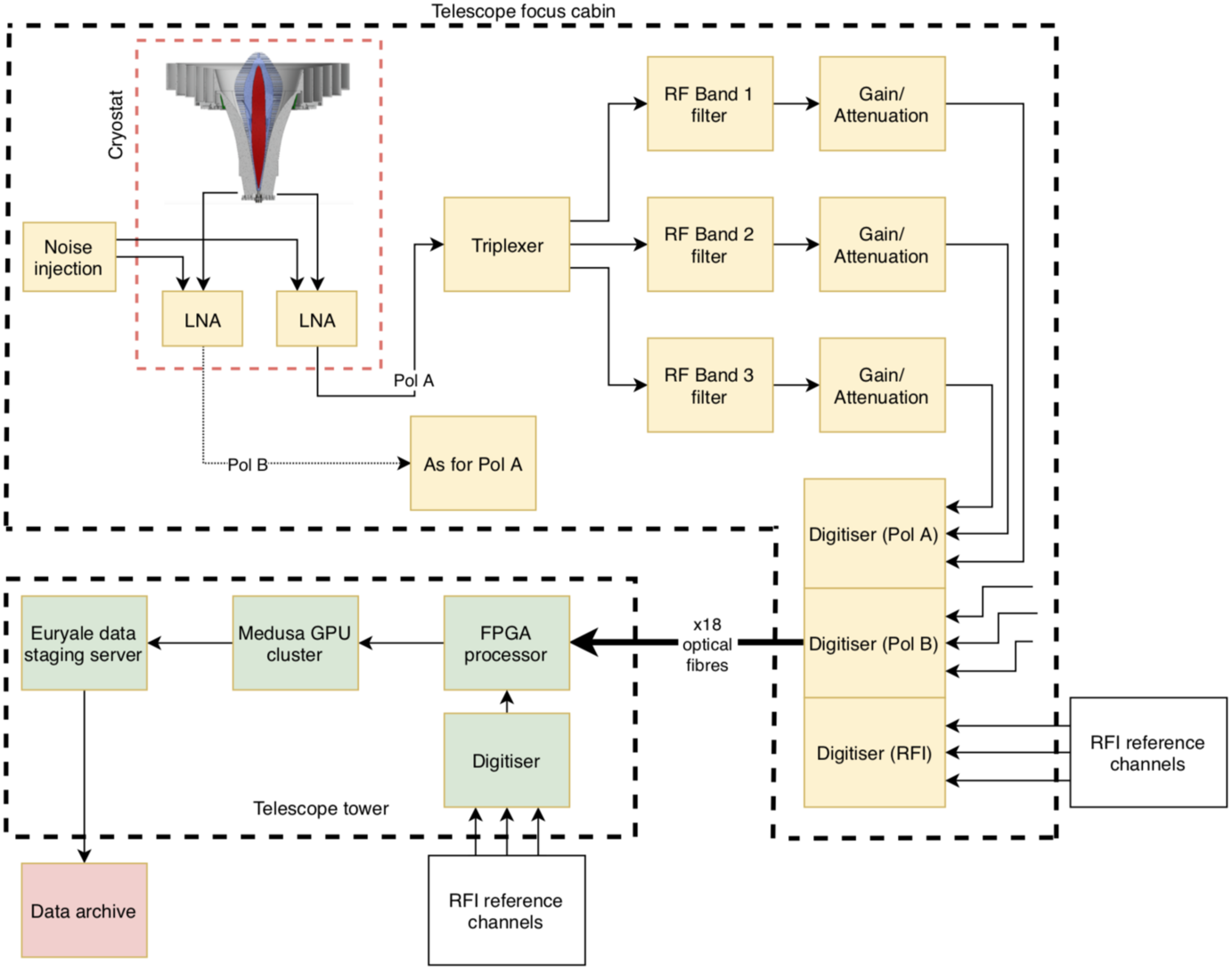
Figure 1. Block diagram of the primary components of the UWL system. Only one polarisation channel is shown for the RF amplifier chain; the other is identical. Note that this figure does not include the monitoring, control nor timing/synchronisation system.
The signal pre-processor system in the tower receives the digitised data and produces critically sampled data streams for 26 sub-bands, each with a 128-MHz bandwidth. The sub-band data streams are passed to an astronomy signal processor system based on Graphics Processor Units (GPUs) known as ‘Medusa’Footnote d that processes each of the sub-bands separately. The processing can involve forming polarisation products, folding these signals at the known period of a pulsar, producing data streams suitable for pulsar and transient searching, or producing high-frequency resolution data sets for the study of spectral lines and the radio continuum background. The output of the astronomy signal processor is transferred to a data-staging server, known as ‘Euryale’Footnote e, that produces archive-ready data products. Astronomers can access the resulting data products from various online archives.
The paper is divided into sections describing the receiver system (Section 2), the signal processing system (Section 3), the timing and synchronisation system (Section 4), the system performance (Section 5), and the RFI environment (Section 6). In the Appendices, we define the terms used in our paper, describe the content of a publicly downloadable data collection, and provide more details on the parameterisation of the receiver system. Finally, we briefly present the author contributions to this work.
2. The receiver system
The receiver system consists of the feed and LNAs, both of which are cryogenically cooled, and the RF amplifier chain. (Dunning et al. Reference Dunning, Bowen, Bourne, Hayman and Smith2015) described the basic properties of the feed. The design is shown in the left-hand panel of Figure 2 and is based on a quad-ridged horn. The middle and right-hand panels of this Figure show different visualisations of the complete receiver package. This design provides a wide bandwidth with comparable performance to narrower band systems by making use of a central dielectric spear to improve the beam properties at high frequencies, and a corrugated skirt to improve the beam properties at low frequencies.
The dielectric spear consists of three layers giving a graded dielectric constant: a central quartz section, a solid polytetrafluoroethylene (PTFE; more commonly known as  $\text{Teflon}^{\text{TM}}$
) section and a slotted PTFE outer section. The feed horn operates over the frequency range
$\text{Teflon}^{\text{TM}}$
) section and a slotted PTFE outer section. The feed horn operates over the frequency range  ${\sim}700$
to
${\sim}700$
to  ${\sim}4.5\,\text{GHz}$
and provides two nominally orthogonal linear polarisations, each with symmetric outputs. The exceptionally wide frequency coverage of the feed required the development of cryogenically cooled LNAs with large dynamic range that cover the entire band. The three-stage LNAs are cooled to 20 K, the feed horn and the dielectric spear are cooled to 70 K, and the outer feed rings are at ambient temperature (because of thermal losses, there is a temperature gradient across the dielectric spear; see Smart et al. Reference Smart, Dunning, Smith, Carter, Bourne, Doherty, Castillo and Dong2019 for more detail). Following the cryogenically cooled LNAs, the signals from the two polarisations are further amplified by ambient temperature amplifiers before digitisation. To assist with the mitigation of RFI, the UWL band for each polarisation is split into three sub-octave RF bands using a triplexer (created using a power splitter and a diplexer) and band-limiting filters. These bands are separately amplified and digitised. As shown in the bottom panel of Figure 3, the three RF bands (labelled Bands 1 to 3) have a relatively flat response over the corresponding digital bands, which cover from 704–1 344, 1 344–2 368, and 2 368–4 032 MHz (see Section 3 for more detail on the digital bands). The separate sub-octave RF bands provide protection against intermodulation products from strong RFI signals affecting other parts of the UWL band. Switchable attenuators allow the choice of signal level for the three RF bands, with RF Band 1 requiring significantly more attenuation than the other two because of the strong RFI in this band. Default attenuator settings ensure that each band normally remains in a linear regime in the presence of RFIFootnote f.
${\sim}4.5\,\text{GHz}$
and provides two nominally orthogonal linear polarisations, each with symmetric outputs. The exceptionally wide frequency coverage of the feed required the development of cryogenically cooled LNAs with large dynamic range that cover the entire band. The three-stage LNAs are cooled to 20 K, the feed horn and the dielectric spear are cooled to 70 K, and the outer feed rings are at ambient temperature (because of thermal losses, there is a temperature gradient across the dielectric spear; see Smart et al. Reference Smart, Dunning, Smith, Carter, Bourne, Doherty, Castillo and Dong2019 for more detail). Following the cryogenically cooled LNAs, the signals from the two polarisations are further amplified by ambient temperature amplifiers before digitisation. To assist with the mitigation of RFI, the UWL band for each polarisation is split into three sub-octave RF bands using a triplexer (created using a power splitter and a diplexer) and band-limiting filters. These bands are separately amplified and digitised. As shown in the bottom panel of Figure 3, the three RF bands (labelled Bands 1 to 3) have a relatively flat response over the corresponding digital bands, which cover from 704–1 344, 1 344–2 368, and 2 368–4 032 MHz (see Section 3 for more detail on the digital bands). The separate sub-octave RF bands provide protection against intermodulation products from strong RFI signals affecting other parts of the UWL band. Switchable attenuators allow the choice of signal level for the three RF bands, with RF Band 1 requiring significantly more attenuation than the other two because of the strong RFI in this band. Default attenuator settings ensure that each band normally remains in a linear regime in the presence of RFIFootnote f.
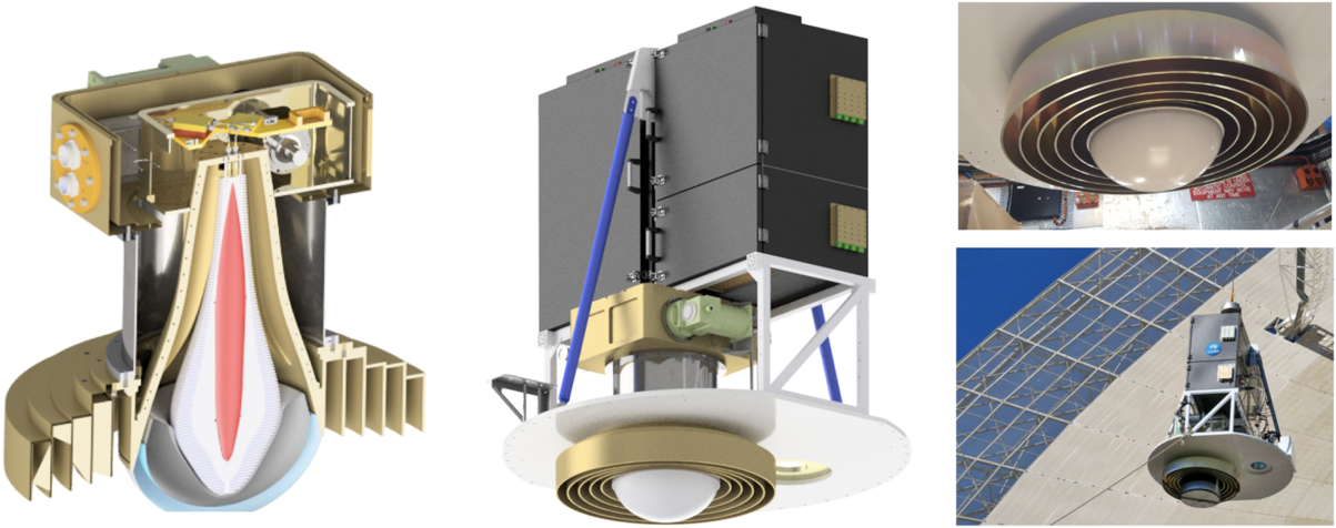
Figure 2. Representation of the feed system: (left) the internal structure of the feed, (centre) the feed, platform, and RF shielded cabinets, and (right) the completed system being installed on the telescope.
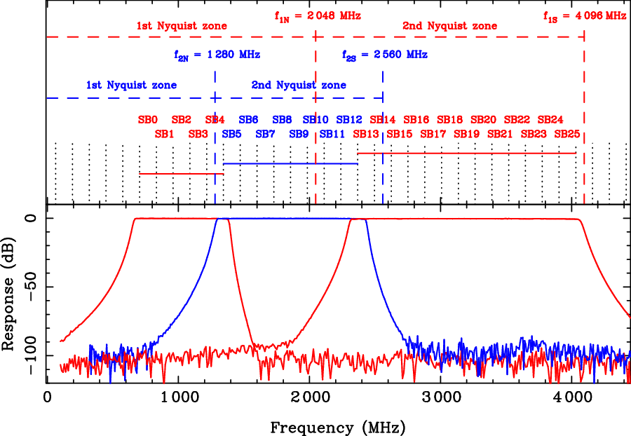
Figure 3. The sampling bands for the UWL. The bottom panel shows the filters determining the three RF bands (RF bands 1, 2, and 3). The digital bands are formed using two sampling frequencies (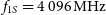 $f_{1S} = 4\,096\,\text{MHz}$
and
$f_{1S} = 4\,096\,\text{MHz}$
and  $f_{2S} = 2\,560\,\text{MHz}$
). These sampling frequencies permit the 26 sub-bands (denoted SBx) each 128 MHz wide. Those shown in red are obtained from the first and second Nyquist zones of
$f_{2S} = 2\,560\,\text{MHz}$
). These sampling frequencies permit the 26 sub-bands (denoted SBx) each 128 MHz wide. Those shown in red are obtained from the first and second Nyquist zones of  $f_{1S}$
. Those in blue are from the second Nyquist zone of
$f_{1S}$
. Those in blue are from the second Nyquist zone of  $f_{2S}$
. See text for further details.
$f_{2S}$
. See text for further details.
A key aspect of the design was to digitise the signals at RF in the focus cabin and then to transmit digital signals to the telescope tower that contains the signal processor instrumentation. The alternative of using analogue RF over fibre for the long ( ${\sim}150\,\text{m}$
) path to the tower was rejected because of potential linearity issues related to the strong RFI, particularly for RF Band 1. Also, analogue transmission over such a long path would be subject to differential delays in the two polarisations with varying ambient conditions, leading to instabilities in derived polarisation parameters.
${\sim}150\,\text{m}$
) path to the tower was rejected because of potential linearity issues related to the strong RFI, particularly for RF Band 1. Also, analogue transmission over such a long path would be subject to differential delays in the two polarisations with varying ambient conditions, leading to instabilities in derived polarisation parameters.
The UWL cannot be rotated (both software and hardware limits are in place to ensure this) and the linear polarisations have been aligned at  $\pm45^\circ$
to the elevation axis of the antenna. The UWL feed design precludes the injection of noise into the feed horn. The artificial noise signal is therefore coupled directly to the inputs of the LNAs. Note that the coupling is non-directional; see Section 5. We also have a capability to radiate noise directly into the feed from a transmitter on the surface of the dish. However, this is currently not used in any standard observing mode. It is possible to vary the amplitude of the injected signal; for the results presented here, the amplitude was between 1 and 2 K across the band.
$\pm45^\circ$
to the elevation axis of the antenna. The UWL feed design precludes the injection of noise into the feed horn. The artificial noise signal is therefore coupled directly to the inputs of the LNAs. Note that the coupling is non-directional; see Section 5. We also have a capability to radiate noise directly into the feed from a transmitter on the surface of the dish. However, this is currently not used in any standard observing mode. It is possible to vary the amplitude of the injected signal; for the results presented here, the amplitude was between 1 and 2 K across the band.
The noise temperature of the LNAs,  $T_{\text{LNA}}$
, was determined using laboratory measurements in a cryogenic test dewar. The results are shown as the solid, cyan line in the upper panel of Figure 4 and is close to 5 K across the entire band. The system temperature (note that, as we are not attempting a rigorous analysis here, we ignore efficiencies and beam pattern weightings) is the sum of several components, which are individually defined below:
$T_{\text{LNA}}$
, was determined using laboratory measurements in a cryogenic test dewar. The results are shown as the solid, cyan line in the upper panel of Figure 4 and is close to 5 K across the entire band. The system temperature (note that, as we are not attempting a rigorous analysis here, we ignore efficiencies and beam pattern weightings) is the sum of several components, which are individually defined below:
 \begin{eqnarray} T_{\text{sys}} &=& T_{\text{rcvr}} + T_{\text{atm}} + T_{\text{Gal}} + T_{\text{CMB}}\nonumber\\ &&+ T_{\text{spill}} + T_{\text{scatt}} + T_{\text{RFI}}. \end{eqnarray}
The  $T_{\text{rcvr}}$
measurements (which include
$T_{\text{rcvr}}$
measurements (which include  $T_{\text{LNA}}$
), also shown in the top panel of Figure 4, were made at the Parkes observatory site with the receiver on the ground facing up, using an ambient temperature absorber as a hot load and the sky as a cold load.
$T_{\text{LNA}}$
), also shown in the top panel of Figure 4, were made at the Parkes observatory site with the receiver on the ground facing up, using an ambient temperature absorber as a hot load and the sky as a cold load.  $T_{\text{rcvr}}$
, which includes contributions from losses in the feed, is
$T_{\text{rcvr}}$
, which includes contributions from losses in the feed, is  ${\sim}9\,\text{K}$
across most of the band, rising from around 3 GHz to
${\sim}9\,\text{K}$
across most of the band, rising from around 3 GHz to  ${\sim}18\,\text{K}$
at
${\sim}18\,\text{K}$
at  ${\sim}4\,\text{GHz}$
.
${\sim}4\,\text{GHz}$
.
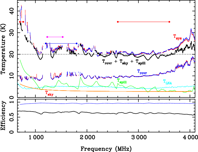
Figure 4. The measured system temperature (T $_{\text{sys}}$
) for the UWL receiver system on the Parkes radio telescope and several of its components are shown in the upper panel. The red and dark blue traces indicate the A and B polarisations, respectively, for
$_{\text{sys}}$
) for the UWL receiver system on the Parkes radio telescope and several of its components are shown in the upper panel. The red and dark blue traces indicate the A and B polarisations, respectively, for  $T_{\text{sys}}$
(upper pair) and
$T_{\text{sys}}$
(upper pair) and  $T_{\text{rcvr}}$
(lower pair). The solid, cyan line (
$T_{\text{rcvr}}$
(lower pair). The solid, cyan line ( ${\sim}5\,\text{K}$
) is the measured
${\sim}5\,\text{K}$
) is the measured  $T_{\text{LNA}}$
, the green line is the estimated
$T_{\text{LNA}}$
, the green line is the estimated  $T_{\text{spill}}$
, and the orange curve (
$T_{\text{spill}}$
, and the orange curve ( ${<}5\,\text{K}$
) is the estimated sky background temperature,
${<}5\,\text{K}$
) is the estimated sky background temperature,  $T_{\text{Gal}} + T_{\text{CMB}}$
. The upper, black line is the sum of the individual estimated noise components. The horizontal dotted line indicates 20 K. The horizontal lines delineated by circles give an approximation to the frequency coverage and system temperature for other receivers available at Parkes. The 10/40cm receiver is represented in red, the 20-cm multibeam receiver in pink, and the H-OH receiver in blue. The lower panel provides measures of the aperture efficiency from laboratory-based measurements and simulation (black line). The higher, blue line in this panel provides an estimate of the main beam efficiency.
$T_{\text{Gal}} + T_{\text{CMB}}$
. The upper, black line is the sum of the individual estimated noise components. The horizontal dotted line indicates 20 K. The horizontal lines delineated by circles give an approximation to the frequency coverage and system temperature for other receivers available at Parkes. The 10/40cm receiver is represented in red, the 20-cm multibeam receiver in pink, and the H-OH receiver in blue. The lower panel provides measures of the aperture efficiency from laboratory-based measurements and simulation (black line). The higher, blue line in this panel provides an estimate of the main beam efficiency.
To determine the expected  $T_{\text{sys}}$
, we assumed an atmospheric contribution (
$T_{\text{sys}}$
, we assumed an atmospheric contribution ( $T_{\text{atm}}$
) of around 2 K at these observing frequencies (Smith Reference Smith1982). The contribution of ‘spillover’ radiation,
$T_{\text{atm}}$
) of around 2 K at these observing frequencies (Smith Reference Smith1982). The contribution of ‘spillover’ radiation,  $T_{\text{spill}}$
, from the ground entering the feed past the main reflector was estimated by integrating the feed response falling outside the reflector, assuming a ground temperature of 290 K. This is shown in Figure 4 as the green line. The relatively large variations are caused by frequency-dependent fluctuations in outer parts of the feed beam pattern.
$T_{\text{spill}}$
, from the ground entering the feed past the main reflector was estimated by integrating the feed response falling outside the reflector, assuming a ground temperature of 290 K. This is shown in Figure 4 as the green line. The relatively large variations are caused by frequency-dependent fluctuations in outer parts of the feed beam pattern.  $T_{\text{scatt}}$
is radiation from any source scattered into the feed from the telescope structure (our modelling does not account for scattering). As far as possible, RFI is eliminated from the signal (see Section 6) and so we do not consider it further in this section.
$T_{\text{scatt}}$
is radiation from any source scattered into the feed from the telescope structure (our modelling does not account for scattering). As far as possible, RFI is eliminated from the signal (see Section 6) and so we do not consider it further in this section.
The sky temperature depends upon the Galactic location being observed. An estimate of  $T_{\text{Gal}}$
was obtained from the reprocessed Haslam et al. (Reference Haslam, Salter, Stoffel and Wilson1982) 408-MHz image of Remazeilles et al. (Reference Remazeilles, Dickinson, Banday and Ghosh2015) for the approximate sky position relevant to the measurements and assuming a spectral index of −2.6 (see range of values in Lawson et al. Reference Lawson, Mayer, Osborne and Parkinson1987 for more details). Note that both the Haslam et al. (Reference Haslam, Salter, Stoffel and Wilson1982) and Remazeilles et al. (Reference Remazeilles, Dickinson, Banday and Ghosh2015) image scales include the cosmic microwave background contribution,
$T_{\text{Gal}}$
was obtained from the reprocessed Haslam et al. (Reference Haslam, Salter, Stoffel and Wilson1982) 408-MHz image of Remazeilles et al. (Reference Remazeilles, Dickinson, Banday and Ghosh2015) for the approximate sky position relevant to the measurements and assuming a spectral index of −2.6 (see range of values in Lawson et al. Reference Lawson, Mayer, Osborne and Parkinson1987 for more details). Note that both the Haslam et al. (Reference Haslam, Salter, Stoffel and Wilson1982) and Remazeilles et al. (Reference Remazeilles, Dickinson, Banday and Ghosh2015) image scales include the cosmic microwave background contribution,  $T_{\text{CMB}}$
, and so this was subtracted from the image value before scaling to the required frequency. All these contributions have been plotted in the upper panel of Figure 4 with the summation being shown as the upper, solid, black line.
$T_{\text{CMB}}$
, and so this was subtracted from the image value before scaling to the required frequency. All these contributions have been plotted in the upper panel of Figure 4 with the summation being shown as the upper, solid, black line.
The measured on-telescope system temperature ( $T_{\text{sys}}$
) as a function of frequency is shown in the top panel of Figure 4 and tabulated in Table 1. These measurements were obtained by comparing spectra obtained with an ambient temperature absorber over the feed with spectra obtained when observing the sky. The
$T_{\text{sys}}$
) as a function of frequency is shown in the top panel of Figure 4 and tabulated in Table 1. These measurements were obtained by comparing spectra obtained with an ambient temperature absorber over the feed with spectra obtained when observing the sky. The  $T_{\text{sys}}$
measurements were carried out with the telescope pointed at the zenith when both the Sun and the Galactic centre were below the horizon (between UTC 12:00 and 20:00 each day over the period 2018 October 29 to 2018 October 31). The
$T_{\text{sys}}$
measurements were carried out with the telescope pointed at the zenith when both the Sun and the Galactic centre were below the horizon (between UTC 12:00 and 20:00 each day over the period 2018 October 29 to 2018 October 31). The  $T_{\text{sys}}$
values match, or significantly improve on, all current and previous Parkes receivers covering the same observing bands (see horizontal bars in Figure 4). The predicted
$T_{\text{sys}}$
values match, or significantly improve on, all current and previous Parkes receivers covering the same observing bands (see horizontal bars in Figure 4). The predicted  $T_{\text{sys}}$
(from Equation (A1) is within a few Kelvin of the measured value over most of the band, with slightly larger discrepancies at the low and high ends. At the low end, the discrepancy could easily be accounted by a small underestimation of the spillover. At the high end, it may result from scattered power from various sources, including the telescope structure itself, entering the feed and/or leakage of ground radiation through the outer parts of the reflector. We note that these
$T_{\text{sys}}$
(from Equation (A1) is within a few Kelvin of the measured value over most of the band, with slightly larger discrepancies at the low and high ends. At the low end, the discrepancy could easily be accounted by a small underestimation of the spillover. At the high end, it may result from scattered power from various sources, including the telescope structure itself, entering the feed and/or leakage of ground radiation through the outer parts of the reflector. We note that these  $T_{\text{sys}}$
measurements were determined from the output of the RF chain and do not include any extra noise contributions from the digitiser and signal processor systems.
$T_{\text{sys}}$
measurements were determined from the output of the RF chain and do not include any extra noise contributions from the digitiser and signal processor systems.
The black line in the bottom panel of Figure 4 shows the expected aperture efficiency for the UWL as installed on the Parkes 64-m telescope. As described by (Smart et al. Reference Smart, Dunning, Smith, Carter, Bourne, Doherty, Castillo and Dong2019), these were determined using laboratory-based measurements of the feed radiation patterns with a model of the telescope. The calculated efficiency is around 65% over the observing band. We compare these results with the astronomically measured efficiencies described below. The upper, blue line in the bottom panel of Figure 4 provides an estimate of the main beam efficiency. These values were also determined from the measured feed patterns using Equation (A7). Across most of the band, the mean main beam efficiency is  ${\sim}0.96$
, reducing to
${\sim}0.96$
, reducing to  ${\sim}0.92$
at the low-frequency end of the band.
${\sim}0.92$
at the low-frequency end of the band.
3. The signal processing systems
The two polarisation channels for each of the three bands are digitised in the focus cabinFootnote g. The analogue-to-digital converters (ADCs) provide 12-bit resolution samples that are formatted into serial data streams complying with the JESD204B (Joint Electron Device Engineering Council Standard Document 204 Revision B) protocol for serially connected data converters. These signals are transported to the signal processors in the telescope tower via single-mode optical fibres, with two fibres required per digitiserFootnote h. The ADCs operate at one of two separate sampling frequencies, 2 560 and 4 096 MHz, to ensure unbroken frequency coverage of the observing band from 704 to 4 032 MHz, as is shown in Figure 3.
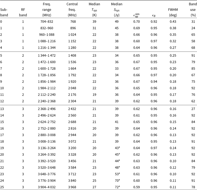
Table 1. Parameters for the 26 UWL sub-bands: the corresponding RF band that feeds them (column 2); sub-band frequency ranges (column 3); the central observing frequency (column 4); the median system temperature (column 5) and system equivalent flux densities as determined using PKS B0407–658 (column 6) summed over both polarisations; an estimate of the antenna (column 7) and main beam (column 8) efficiencies, the full-width half-maximum (FWHM) of the measured beam shape (column 9), and the fraction of the sub-band containing useful data (column 10, see main text for definition).
The six digitiser data streams (nine when the focus cabin RFI reference signal is implemented, see Section 7) are fed to a pre-processor unit in the telescope tower which utilises Field Programmable Gate Arrays (FPGAs) to implement polyphase frequency channelisers that produce 26 contiguous sub-bands each 128 MHz wide for each polarisation (see Table 1). The pre-processor subsystem is built around a commercial platform with a Xilinx® Kintex® UltrascaleTM FPGA and eight Quad Small Form-factor Pluggable cages for data exchange. Each FPGA board receives data from two ADCs and eight such boards are housed in custom-made enclosures totalling eight rack units. The total designed capacity is 32 GHz (256 channels of 128 MHz) of real-time processing bandwidth and 1.28 Tb  $\text{s}^{-1}$
of Ethernet data output.
$\text{s}^{-1}$
of Ethernet data output.
Currently, each sub-band delivered by the pre-processor is produced using a critically sampled polyphase filterbank. To eliminate the effects of aliasing at the sub-band edges, an oversampled polyphase filterbank is planned, but has not yet been implemented. There are two separate versions of the FPGA signal processing firmware to match the two ADC sampling frequencies. The primary differences between the two firmware versions are the number of output sub-bands and the length of the finite impulse response (FIR) filter for the polyphase channelisers. For the 4 096-MHz sample clock firmware, there are 16 output sub-bands and 1 024 coefficients in the channeliser filter. For the 2 560-MHz sample clock, there are 10 output sub-bands and 640 coefficients in the channeliser filter. The channeliser FIR filters are carefully designed to achieve the best balance between passband flatness and attenuation of out-of-band components while also maintaining steep transition bands to minimise gain loss at the sub-band edges and aliasing between sub-bands. The FIR filters are designed using a least squares algorithm with a Kaiser window function to smooth the resulting impulse response and have a passband ripple of  ${\sim}0.02\,\text{dB}$
with a transition at the band edges crossing the adjacent sub-band at −6 dB. The relationship of the sub-band frequencies to ADC sampling frequencies is illustrated in the top panel of Figure 3 and tabulated in Table 1.
${\sim}0.02\,\text{dB}$
with a transition at the band edges crossing the adjacent sub-band at −6 dB. The relationship of the sub-band frequencies to ADC sampling frequencies is illustrated in the top panel of Figure 3 and tabulated in Table 1.
The polyphase filterbank is designed to preserve full numerical precision throughout both the FIR and Fast Fourier Transform (FFT) stages. Accordingly, there is ‘bit-growth’ from the input 12 bits from the ADCs to 23 bits at the filterbank sub-band outputs. A number representation of 23 bits is not compatible with a CPU/GPU computational environment and would also require significant additional network infrastructure to transport. For these reasons, a scaling module is implemented for each sub-band output to reduce the number representation down to 16 bits (signed two’s-complement). This scaling operation is an area where dynamic range issues of numerical overflow, underflow, or saturation can occur, so the location of the 16 bits that are selected from the input 23 can be controlled through software-adjustable fixed gain that has eight settings ranging exponentially from unity gain through to a gain of 128.
The output data streams from the FPGA pre-processor are sent as multicast Ethernet packets as 10 Gb  $\text{s}^{-1}$
Ethernet (10 GbE) to a 64-port Cisco® 3164Q network switch (they are aggregated as
$\text{s}^{-1}$
Ethernet (10 GbE) to a 64-port Cisco® 3164Q network switch (they are aggregated as  $4\,\times\,10\,\text{GbE}$
on a 40-GbE port on the switch). During observations, the GPU-based Medusa signal processor subscribes to the multicast streams and runs further processing on them to form science data products, as described below. For the UWL RF bands, the FPGA signal processor outputs data as User Datagram Protocol (UDP) packets of size 8 272 B, each containing a single ‘Data Frame’, as defined in the VLBI Data Interchange Format (Whitney et al. Reference Whitney, Kettenis, Phillips and Sekido2009) specification (VDIF; http://www.vlbi.org/vdif/). The FPGA pre-processor outputs a total of 52 VDIF UDP streams, one for each polarisation of each sub-band, with 128 MHz bandwidth using complex sampling and 16-bit resolution per complex component; the total ingest data rate at the switch is 215 Gb
$4\,\times\,10\,\text{GbE}$
on a 40-GbE port on the switch). During observations, the GPU-based Medusa signal processor subscribes to the multicast streams and runs further processing on them to form science data products, as described below. For the UWL RF bands, the FPGA signal processor outputs data as User Datagram Protocol (UDP) packets of size 8 272 B, each containing a single ‘Data Frame’, as defined in the VLBI Data Interchange Format (Whitney et al. Reference Whitney, Kettenis, Phillips and Sekido2009) specification (VDIF; http://www.vlbi.org/vdif/). The FPGA pre-processor outputs a total of 52 VDIF UDP streams, one for each polarisation of each sub-band, with 128 MHz bandwidth using complex sampling and 16-bit resolution per complex component; the total ingest data rate at the switch is 215 Gb  $\text{s}^{-1}$
.
$\text{s}^{-1}$
.
The use of multicast Ethernet allows copies of the data to be sent not only to Medusa, but also to the Breakthrough Listen (BL) data recorder (Price et al. Reference Price2018). Data are transported from the UWL switch to the BL switch via eight 40 GbE links, which are configured as an aggregated group using Link Aggregration Control Protocol.
3.1. The Medusa GPU cluster
Medusa consists of nine rack-mounted, server-class machines, each equipped with dual Intel Xeon CPUs, 128 GB of random access memory (RAM), two 40 Gb  $\text{s}^{-1}$
Network Interface Cards (NICs), four NVIDIA Titan X GPUs, and an array of Solid State Disks. The 26 sub-bands are distributed across the nine Medusa servers, with each dual polarisation sub-band being received into a large, shared memory, Pulsar Distributed Acquisition and Data Analysis (PSRDADA) (http://psrdada.sourceforge.net/) ring buffer. The sub-bands are then processed independently on the GPUs to form the desired astronomical data products. The spip (http://github.com/ajameson/spip) and dspsr (van Straten & Bailes Reference van Straten and Bailes2011) software libraries are used to form the output data products for pulsar timing, pulsar searching or single-pulse studies, transient searching, spectral line and continuum studies and/or VLBI. These are written to the local file systems and then transferred via a 40 Gb
$\text{s}^{-1}$
Network Interface Cards (NICs), four NVIDIA Titan X GPUs, and an array of Solid State Disks. The 26 sub-bands are distributed across the nine Medusa servers, with each dual polarisation sub-band being received into a large, shared memory, Pulsar Distributed Acquisition and Data Analysis (PSRDADA) (http://psrdada.sourceforge.net/) ring buffer. The sub-bands are then processed independently on the GPUs to form the desired astronomical data products. The spip (http://github.com/ajameson/spip) and dspsr (van Straten & Bailes Reference van Straten and Bailes2011) software libraries are used to form the output data products for pulsar timing, pulsar searching or single-pulse studies, transient searching, spectral line and continuum studies and/or VLBI. These are written to the local file systems and then transferred via a 40 Gb  $\text{s}^{-1}$
NIC to the Euryale data-staging server.
$\text{s}^{-1}$
NIC to the Euryale data-staging server.
For all astronomy modes and all sub-bands, Medusa first performs signal processing tasks, such as unpacking the VDIF data streams from the FPGA pre-processor and converting the signals to upper sideband (increasing sky frequency with channel number). Optional functions include the ability to adaptively mitigate RFI if a reference RFI data stream is available, and the formation of calibration spectra if a switched noise source is operating. After this initial processing, each 128-MHz sub-band is passed to the primary signal processing system, which produces the requested astronomy data products.
Pulsar-related (search and fold mode) processing tasks have been developed around the dspsr software suite (van Straten & Bailes Reference van Straten and Bailes2011). Coherent de-dispersion can be applied to both pulsar fold- and search-mode observations. Such de-dispersion removes the intra-channel dispersive delays, but not the inter-channel delays.
The specific astronomical observing modes, which may be independently configured for each of the 26 sub-bands, are as follows:
Pulsar folding:dspsr acquires the pulsar ephemerides from a copy of the Australia Telescope National Facility (ATNF) Pulsar Catalogue (Manchester et al. Reference Manchester, Hobbs, Teoh and Hobbs2005) and user-generated pulsar parameters and uses the tempo2 software package (Hobbs, Edwards & Manchester Reference Hobbs, Edwards and Manchester2006) to predict the pulse topocentric period and phase. The voltage data are channelised (between 64 and 4 096 channels in standard observing modes) with each channel coherently de-dispersed using a convolving filterbank algorithm. The data are then detected (the channelised voltages are converted to power) and polarisation products formed, folded into pulsar phase bins (between 8 and 4 096) synchronously with the topocentric pulsar period and integrated to the desired sub-integration length (currently between 8 and 60 s). Either one, two, or four polarisation products, respectively, $\text{AA}^*+\text{BB}^*$
(pseudo-Stokes I);
$\text{AA}^*$
,
$\text{BB}^*$
; and
$\text{AA}^*$
,
$\text{BB}^*$
, Real(
$\text{A}^*\text{B}$
), Imag(
$\text{A}^*\text{B}$
), where A and B are the two orthogonal polarisation signals and the
$^*$
symbol indicates the complex conjugate, can be formed and recorded. The sub-integration data are then added to a PSRFITS (Hotan, van Straten & Manchester Reference Hotan, van Straten and Manchester2004) fold-mode file as 16 bit values. A typical observation in this mode would have 128 channels per sub-band, 1 024 phase bins, 4 polarisation products, and 30-s subintegration lengths. This leads to a data rate of around 27 MB per subintegration or
${\sim}3\,\text{GB}$
for a 1-h observation.
$\text{AA}^*+\text{BB}^*$
(pseudo-Stokes I);
$\text{AA}^*$
,
$\text{BB}^*$
; and
$\text{AA}^*$
,
$\text{BB}^*$
, Real(
$\text{A}^*\text{B}$
), Imag(
$\text{A}^*\text{B}$
), where A and B are the two orthogonal polarisation signals and the
$^*$
symbol indicates the complex conjugate, can be formed and recorded. The sub-integration data are then added to a PSRFITS (Hotan, van Straten & Manchester Reference Hotan, van Straten and Manchester2004) fold-mode file as 16 bit values. A typical observation in this mode would have 128 channels per sub-band, 1 024 phase bins, 4 polarisation products, and 30-s subintegration lengths. This leads to a data rate of around 27 MB per subintegration or
${\sim}3\,\text{GB}$
for a 1-h observation.Pulsar searching: The dspsr package includes digifits, which processes the sub-band voltage data to produce a set of PSRFITS search-mode data files. The data are channelised (8 to 4 096 channels) and one, two, or four polarisation products formed as for fold mode. These are averaged to a specified sampling interval (
${\sim}1 \mu\text{s}$
to 1 s) and then they are rescaled to zero mean and unit variance using a computed scale and offset. These normalised samples are scaled and requantised to 1-, 2-, 4-, or 8-bit values (Jenet & Anderson Reference Jenet and Anderson1998). The offset and scale are retained for each block of samples (typically 4 096 samples) and recorded with the time series data allowing for reconstruction of the original signal. The data volume and rate can vary enormously, depending upon the chosen parameters. For instance, for an observation with a sampling rate of
$64\mu\text{s}$
, 1 024 channels/sub-band, 2-bit sampling, and 1-polarisation product (typical for recent surveys), the data rate would be 100 MB
$\text{s}^{-1}$
or 370 GB for a 1-h observation. However, to deal with dispersion smearing, an observer may wish to observe with significantly narrower channel bandwidths for the low-frequency sub-bands and wider bandwidths for the high-frequency sub-bands.Pulsar single-pulse studies and searches at a known dispersion measure (DM): If the DM of an observed pulsar is known, or if a pulsar search is being carried out with prior knowledge of the likely DM for any pulsar (or similarly, for searching for repeated fast radio burst events), then it is possible to coherently de-disperse the search-mode data stream and to produce PSRFITS search-mode data files. This allows for substantially reduced frequency resolution, which may then be traded for higher time resolution. The data rate in this mode depend upon the chosen number of channels. If the pulsar DM is well known then, in theory, only a few channels are required for each sub-band, but having only a few channels can make RFI flagging challenging. A typical observation mode may have
$32\hbox{-}\mu\text{s}$
sampling, 8-bit samples, four polarisation products and 128 channels for each sub-band. This produces 400 MB
$\text{s}^{-1}$
or 1.5 TB in a 1-h observation.Spectral line and continuum observations: The data are channelised with up to
$2^{21} = 2\,097\,152$
channels per sub-band (equivalent to a frequency resolution of 61 Hz) forming one, two, or four polarisation products as for pulsar modes, with a sampling interval between 0.25 and 60 s. These spectra are stored in Single-Dish Hierarchical Data Format (SDHDF; see below). If available, calibration spectra may be stored in each output data file. Zoom bands will soon be supported by forming spectra spanning entire sub-bands at the desired frequency resolution and then discarding unwanted channels before the final data product is formed. One restriction of the UWL system is that the digitiser sampling frequencies are fixed. It is therefore not possible to calibrate the bandpass by frequency switching. As above, the data rate can vary enormously, depending on the chosen parameters. With
$2^{21}$
channels per sub-band, the data rate is 436 MB for each spectrum written to disc. If one spectrum is produced each second, then this corresponds to
$1.6\,\text{TB \, h}^{-1}$
.


The switched noise source, used to provide a calibration signal, can be synchronised with the signal processing system with an observer-selected switching frequency. Medusa can then produce separate calibrator-on and calibrator-off spectra, currently implemented for calibration of spectral data. Planned upgrades will enable the user to select the type of injected calibration signal and its frequency, phase and duty cycle (see Section 7).
3.2. Data staging and archiving
The specifications for the data-staging server, Euryale, were defined so that it could receive the incoming data streams, manipulate the data files, interface with databases containing relevant information such as telescope pointing directions, have a disc buffer to store the data files, and the ability to transfer the completed data files to the data archives.
To optimise performance, the incoming data streams are balanced between two 40 Gb  $\text{s}^{-1}$
network cards, four (non-volatile memory express; NVMe) discs (each
$\text{s}^{-1}$
network cards, four (non-volatile memory express; NVMe) discs (each  ${\sim}4\,\text{TB}$
in size) and two Intel Xeon CPUs each with eight cores and two threads per core. The data files can be large and the system needs to manipulate (including re-ordering and averaging) large data volumes so the Euryale server has 376 GB of RAM. The server produces archive-ready data products by combining the data files from each of the sub-bands, including calibration data, applying observational metadata, and writing out files in the required data format. The completed data products are temporarily stored on a large Redundant Array of Independent Disks (RAID) storage unit (this RAID provides a usable
${\sim}4\,\text{TB}$
in size) and two Intel Xeon CPUs each with eight cores and two threads per core. The data files can be large and the system needs to manipulate (including re-ordering and averaging) large data volumes so the Euryale server has 376 GB of RAM. The server produces archive-ready data products by combining the data files from each of the sub-bands, including calibration data, applying observational metadata, and writing out files in the required data format. The completed data products are temporarily stored on a large Redundant Array of Independent Disks (RAID) storage unit (this RAID provides a usable  ${\sim}86\,\text{TB}$
data store). The data files are then sent to the relevant archives.
${\sim}86\,\text{TB}$
data store). The data files are then sent to the relevant archives.
For the spectral line and continuum data sets, we have developed SDHDF, a format based on the Hierarchical Data Format definition (HDF; https://www.hdfgroup.org/) initially used for the HIPSR system at Parkes for recording Hi observations using the 20-cm multibeam receiver (Price et al. Reference Price, Staveley-Smith, Bailes, Carretti, Jameson, Jones, van Straten and Schediwy2016). The SDHDF format is versatile and extendable and able to be readily handled by modern computer languages. We are continuing to develop and define this data format and our final definition will be published elsewhere.
All archive-ready data products need to include metadata for the observation. Euryale collects metadata from the observing systems and the GPU cluster and includes these values in the final data product. We normally ensure that no individual pulsar data file becomes larger than  ${\sim}10\,\text{GB}$
by splitting observation data files in time and/or frequency.
${\sim}10\,\text{GB}$
by splitting observation data files in time and/or frequency.
Data sets for the majority of observations with the Parkes telescope become publicly available after an 18-month proprietary period. The pulsar data sets are available from Commonwealth Scientific and Industrial Research Organisation (CSIRO)’s data archive (https://data.csiro.au; Hobbs et al. Reference Hobbs2011). The spectral line and continuum data sets will be made available from the Australia Telescope Online Archive (ATOA; https://atoa.atnf.csiro.au) or the CSIRO ASKAP Science Data Archive, CASDA (Chapman et al. Reference Chapman, Dempsey, Miller, Heywood, Pritchard, Sangster, Whiting and Dart2017).
4. Timing and synchronisation
An observatory distributed clock system, which is referenced to the observatory’s hydrogen maser frequency standard, is used to derive precise 128-MHz and 1-Hz reference signals for the data acquistion systems. Phase-locked synchronisation signals at 2.56 MHz for the 4 096 MHz system and 1.6 MHz for the 2 560 MHz system, known as ‘SYSREF’ signals, are required by the ADCs. These are derived from the 128-MHz reference signals and distributed with it to the focus cabin over optical fibres. A local synthesiser in the cabin generates the sampling clocks from the 128-MHz reference and distributes them to all ADCs along with a copy of the appropriate SYSREF clock. The combination of the sampling clock, SYSREF and a 1-Hz gated synchronisation from the FPGA receivers, along with local copies of these signals supplied directly to the FPGA, allows for precise, repeatable synchronisation with deterministic latency. The ADCs are synchronised to a chosen SYSREF edge, and therefore the synchronisation error is expected to be sub-nanosecond, relative to the maser standard. Time synchronisation to terrestrial time standards at a level of a few nanoseconds is obtained by measuring the offset between the observatory clock 1-s pulses and those from a Global Positioning System (GPS) receiver. These are subsequently referenced to International Atomic Time (TAI) or other time standards using time offsets published by the Bureau International des Poids et Mesures (BIPM)Footnote i.
To illustrate the timing stability of the UWL system, Figure 5 shows the pulsar timing residuals for PSR J1909–3744 in the 10-cm observing band. This is the most stable pulsar observed by the PPTA project (Manchester et al. Reference Manchester2013). The residuals in black were obtained using the 10-cm receiver and the PDFB4 processor. Those in red are for an identical band, but obtained through the UWL system. The rms of the timing residuals (that span around 6 months) obtained with the Medusa system (over this relatively small band) is 145 ns and the residuals are dominated by the uncertainty on their measurement. The UWL is clearly adequate for high-precision pulsar timing, but we will continue to test the timing precision and accuracy of the system and to improve our knowledge of the delays between this system and earlier receiver and signal processor combinations. Our intention is to determine the absolute delays required to convert any measured pulse arrival times to the intersection of the axes of the telescope (see Manchester et al. Reference Manchester2013) for details on how this was carried out for the PDFB4 signal processor).
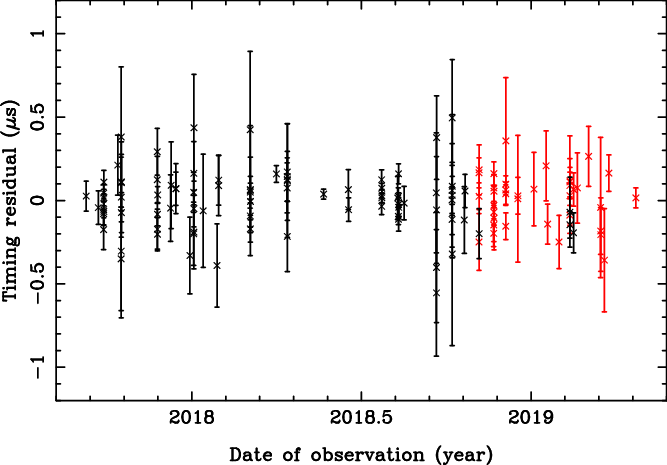
Figure 5. Timing residuals from PSR J1909–3744 obtained by the PPTA project team. Points in black are from observations with the 10-cm receiver and PDFB4 signal processor. Those in red are observations covering the same band, but with the UWL system.
5. System performance
Here, we describe the system performance as measured through the entire system (from the feed to the final data products). Figure 6 shows spectra with a frequency resolution of 488 Hz across the three RF bands. During this 2-min observation, the telescope was pointed towards the zenith. The sub-band spectral shapes are significantly affected by RFI (see Section 6) and quasi-periodic oscillations. For instance, the spectrum contains the characteristic small-scale ripple with a periodicity of  ${\sim}5.7\,\text{MHz}$
(see zoomed region in the figure), which arises from reflections in the 26-m space between the vertex and the underside of the focus cabin. The narrowband spikes in the spectra are not yet fully understood; many will be externally generated RFI, although those at frequencies related to 1 024 and 2 560 MHz are linked to the timing system and sampling frequencies. Band 3 has a currently uncompensated
${\sim}5.7\,\text{MHz}$
(see zoomed region in the figure), which arises from reflections in the 26-m space between the vertex and the underside of the focus cabin. The narrowband spikes in the spectra are not yet fully understood; many will be externally generated RFI, although those at frequencies related to 1 024 and 2 560 MHz are linked to the timing system and sampling frequencies. Band 3 has a currently uncompensated  ${\sim}10\,\text{dB}$
slope across the band which originates in an RF amplifier within the digitiser module. This slope and the sub-band edges are stable and can be calibrated through observations by means of the injected calibration signal.
${\sim}10\,\text{dB}$
slope across the band which originates in an RF amplifier within the digitiser module. This slope and the sub-band edges are stable and can be calibrated through observations by means of the injected calibration signal.

Figure 6. Average spectra across three RF bands obtained on 2019 February 24 at 22:48:23 UTC. The red and blue traces represent the A and B polarisations, respectively. The vertical, dotted lines indicate the sub-band boundaries and the principal RFI transmissions are labelled. The narrow spikes at 1 024, 1 920, and 3 072 MHz are digital processing artefacts related to the clock signals. NBN stands for the National Broadband Network and BT for Bluetooth. The zoomed region in RF Band 2 highlights a characteristic ripple that is described in the text. The main text also provides an explanation of the slope across RF Band 3.
The system equivalent flux density for the telescope with this receiver system ( $S_{\text{sys}}$
) and the calibrator source (
$S_{\text{sys}}$
) and the calibrator source ( $S_{\text{cal}}$
) were determined by observing PKS B0407–658 and its surroundings (we note that we obtain almost identical results with the calibrator PKS B1934–638). Each observation lasted 2 min at positions
$S_{\text{cal}}$
) were determined by observing PKS B0407–658 and its surroundings (we note that we obtain almost identical results with the calibrator PKS B1934–638). Each observation lasted 2 min at positions  $1^\circ$
North of PKS B0407–658, pointed directly at the source,
$1^\circ$
North of PKS B0407–658, pointed directly at the source,  $1^\circ$
to the South, again pointing at the source, and then again to the North. During each observation, the noise injection is switched at a frequency of 11.123 Hz. The data were processed using the Psrchive program fluxcal to produce flux calibration files for each band. This process assumes that PKS B0407–658 has a flux density of 15.4 Jy at 1 400 MHz and a spectral index of −1.20 over the entire band (obtained from the Australia Telescope Compact Array calibrator databaseFootnote j). The measured
$1^\circ$
to the South, again pointing at the source, and then again to the North. During each observation, the noise injection is switched at a frequency of 11.123 Hz. The data were processed using the Psrchive program fluxcal to produce flux calibration files for each band. This process assumes that PKS B0407–658 has a flux density of 15.4 Jy at 1 400 MHz and a spectral index of −1.20 over the entire band (obtained from the Australia Telescope Compact Array calibrator databaseFootnote j). The measured  $S_{\text{sys}}$
and
$S_{\text{sys}}$
and  $S_{\text{cal}}$
values as a function of frequency are shown in the upper and lower panels of Figure 7, respectively. The lower red and blue lines in each panel of the figure show the determinations independently for each polarisation. The upper, black line in the top panel is the more commonly quoted summation of both polarisations. The median
$S_{\text{cal}}$
values as a function of frequency are shown in the upper and lower panels of Figure 7, respectively. The lower red and blue lines in each panel of the figure show the determinations independently for each polarisation. The upper, black line in the top panel is the more commonly quoted summation of both polarisations. The median  $S_{\text{sys}}$
values for each sub-band are listed in Table 1.
$S_{\text{sys}}$
values for each sub-band are listed in Table 1.
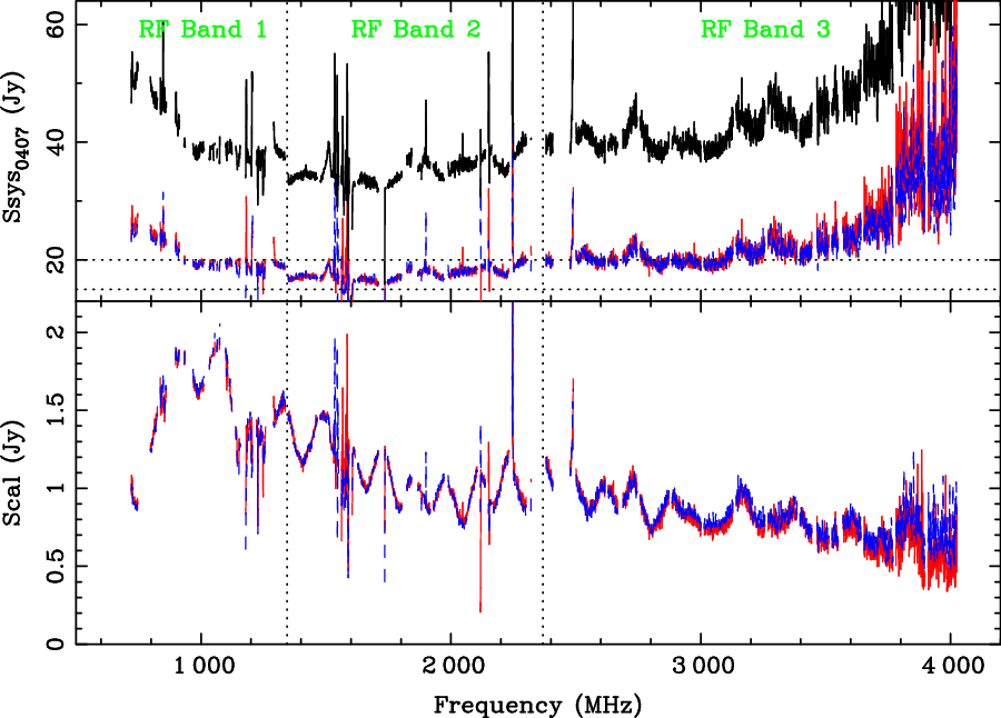
Figure 7. The measured system equivalent flux density ( $\text{S}_{\text{sys}}$
) for the UWL receiver system on the Parkes radio telescope is shown in the upper panel, where the red and blue traces indicate the A and B polarisations, respectively, and the black line is the sum of the two polarisations. These measurements were obtained using observations of PKS 0407–658. The step between RF bands 1 and 2 is discussed in the text. The equivalent flux density of the injected calibration signal (
$\text{S}_{\text{sys}}$
) for the UWL receiver system on the Parkes radio telescope is shown in the upper panel, where the red and blue traces indicate the A and B polarisations, respectively, and the black line is the sum of the two polarisations. These measurements were obtained using observations of PKS 0407–658. The step between RF bands 1 and 2 is discussed in the text. The equivalent flux density of the injected calibration signal ( $\text{S}_{\text{cal}}$
) for each polarisation is shown in the lower panel.
$\text{S}_{\text{cal}}$
) for each polarisation is shown in the lower panel.
Whereas the  $T_{\text{sys}}$
measurements, described in Section 2, were obtained from the output of the receiver system, while the telescope was pointing at zenith, the
$T_{\text{sys}}$
measurements, described in Section 2, were obtained from the output of the receiver system, while the telescope was pointing at zenith, the  $S_{\text{sys}}$
measurements have been determined using an astronomical source through the entire UWL system (including the digitisers, FPGAs, and GPU processors). The discontinuous break in the
$S_{\text{sys}}$
measurements have been determined using an astronomical source through the entire UWL system (including the digitisers, FPGAs, and GPU processors). The discontinuous break in the  $S_{\text{sys}}$
measurements seen between RF bands 1 and 2 in Figure 7 results from the extra attenuation required in Band 1 to avoid saturation effects in the analogue or digital systems which could otherwise occur because of the very strong mobile phone transmitters in this bandFootnote k. As Figure 6 shows, these transmitters can be up to 50 dB above the receiver noise floor. However, this extra attenuation results in a significant digitiser noise contribution, adding an extra
$S_{\text{sys}}$
measurements seen between RF bands 1 and 2 in Figure 7 results from the extra attenuation required in Band 1 to avoid saturation effects in the analogue or digital systems which could otherwise occur because of the very strong mobile phone transmitters in this bandFootnote k. As Figure 6 shows, these transmitters can be up to 50 dB above the receiver noise floor. However, this extra attenuation results in a significant digitiser noise contribution, adding an extra  ${\sim}3\,\text{Jy}$
to the measured system equivalent flux density.
${\sim}3\,\text{Jy}$
to the measured system equivalent flux density.
The  $S_{\text{cal}}$
values clearly contain an oscillation with a
$S_{\text{cal}}$
values clearly contain an oscillation with a  ${\sim}100\,\text{MHz}$
periodicity. The noise source is injected into the LNA system, but the coupler is not directional. This oscillation is believed to result from reflection off the tip of the dielectric spear. The oscillation period and structure are stable and, to date, have not affected the calibration of astronomical data sets.
${\sim}100\,\text{MHz}$
periodicity. The noise source is injected into the LNA system, but the coupler is not directional. This oscillation is believed to result from reflection off the tip of the dielectric spear. The oscillation period and structure are stable and, to date, have not affected the calibration of astronomical data sets.
Using Equation (A6) in Appendix A, we can obtain estimates for the aperture efficiency,  $\epsilon_{\text{ap}}$
, from the system equivalent flux density values and the system temperature values (Figure 7). We note that the
$\epsilon_{\text{ap}}$
, from the system equivalent flux density values and the system temperature values (Figure 7). We note that the  $\text{T}_{\text{sys}}$
measurements were obtained at nighttime, with the telescope pointing at zenith using an independent spectrum analyser and hence do not include extra noise from the digitisers. However, the
$\text{T}_{\text{sys}}$
measurements were obtained at nighttime, with the telescope pointing at zenith using an independent spectrum analyser and hence do not include extra noise from the digitisers. However, the  $S_{\text{sys}}$
measurements were obtained with a telescope zenith angle of
$S_{\text{sys}}$
measurements were obtained with a telescope zenith angle of  $40^\circ$
(elevation angle of
$40^\circ$
(elevation angle of  $50^\circ$
). We, therefore, have extra contributions to
$50^\circ$
). We, therefore, have extra contributions to  $\text{T}_{\text{sys}}$
from the atmosphere, spillover, and from the digitiser system. For a typical sub-band (we have chosen sub-band 5 spanning from 1 344 to 1 472 MHz), we estimate an extra contribution to
$\text{T}_{\text{sys}}$
from the atmosphere, spillover, and from the digitiser system. For a typical sub-band (we have chosen sub-band 5 spanning from 1 344 to 1 472 MHz), we estimate an extra contribution to  $\text{T}_{\text{sys}}$
during the PKS 0407–658 observations of
$\text{T}_{\text{sys}}$
during the PKS 0407–658 observations of  ${\sim}4\,\text{K}$
giving
${\sim}4\,\text{K}$
giving  $\epsilon_{\text{ap}} \approx 0.7$
. From Equation (A5) in Appendix A, this converts to a gain of
$\epsilon_{\text{ap}} \approx 0.7$
. From Equation (A5) in Appendix A, this converts to a gain of  $G_{\text{DPFU}}\sim 0.8\,\text{K \,Jy}^{-1}$
.
$G_{\text{DPFU}}\sim 0.8\,\text{K \,Jy}^{-1}$
.
The feed has been designed to have a constant beam width across the band (Smart et al. Reference Smart, Dunning, Smith, Carter, Bourne, Doherty, Castillo and Dong2019). However, the telescope beam width as measured on the sky remains proportional to the observing wavelength. Theoretical full-width half-power beam widths calculated from  $1.02\lambda/D$
(where
$1.02\lambda/D$
(where  $\lambda$
is the observing wavelength and D, the telescope diameter) give 23, 12, and 4 arcmin for 700, 1 400, and 4 032 MHz, respectively. A high dynamic range measurement of the actual beam shape over the wide band can be obtained by determining the flux density (Stokes I) of the Vela pulsar (PSR J0835–4510) as a function of the angular separation between the known pulsar position and the telescope pointing direction (we define the pointing in azimuth, A, and elevation, E). We have carried out multiple observations of Vela with the telescope offset in a grid of (
$\lambda$
is the observing wavelength and D, the telescope diameter) give 23, 12, and 4 arcmin for 700, 1 400, and 4 032 MHz, respectively. A high dynamic range measurement of the actual beam shape over the wide band can be obtained by determining the flux density (Stokes I) of the Vela pulsar (PSR J0835–4510) as a function of the angular separation between the known pulsar position and the telescope pointing direction (we define the pointing in azimuth, A, and elevation, E). We have carried out multiple observations of Vela with the telescope offset in a grid of ( $A \cos E$
, E) positions. Figure 8 shows representative beam shapes (for sub-band 5 and centred on 1 408 MHz). The complete set of beam shape data files is available for download (see Appendix B). The results from the grid pointings in elevation and in azimuth are not identical. This is primarily caused by the presence of a feed leg in the elevation plane. We overlay predictions of the beam shape obtained from electromagnetic simulations. The blue dashed lines are an ideal case with no attempt to model the effect of the prime focus cabin. The red, dashed line includes a simplified model of the cabin (assumed to be a circular blockage), but does not include the effect of the feed cabin support legs. We do not expect a perfect match between the observing beam shape and the prediction, but note that they match remarkably well and that the sidelobe structure is dominated by the effect of the focus cabin. Data files containing the predictions are also available as part of our public data collection.
$A \cos E$
, E) positions. Figure 8 shows representative beam shapes (for sub-band 5 and centred on 1 408 MHz). The complete set of beam shape data files is available for download (see Appendix B). The results from the grid pointings in elevation and in azimuth are not identical. This is primarily caused by the presence of a feed leg in the elevation plane. We overlay predictions of the beam shape obtained from electromagnetic simulations. The blue dashed lines are an ideal case with no attempt to model the effect of the prime focus cabin. The red, dashed line includes a simplified model of the cabin (assumed to be a circular blockage), but does not include the effect of the feed cabin support legs. We do not expect a perfect match between the observing beam shape and the prediction, but note that they match remarkably well and that the sidelobe structure is dominated by the effect of the focus cabin. Data files containing the predictions are also available as part of our public data collection.
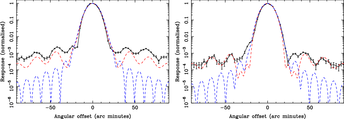
Figure 8. Beam pattern obtained through scans in azimuth (left) and elevation (right) for the 20-cm observing band (sub-band 5, Table 1). The measured response is shown using the black line and error bars. The red and blue dashed lines are modelled beam shapes that are described in the text.
The on-axis polarimetric response of the receiver system is modelled using an updated version of the Measurement Equation Modeling (MEM) technique originally described in (van Straten Reference van Straten2004). The required updates, motivated by (Liao et al. Reference Liao, Chang, Kuo, Masui, Oppermann, Pen and Peterson2016), remove the assumption that the system noise has insignificant circular polarisation and enable modelling of an artificial noise source that is coupled after the feed. We have used this updated MEM algorithm to measure the properties of the receiver (including the differential gain, differential phase, and cross-coupling of the receptors; and the Stokes parameters of the artificial calibration signal). As inputs, we observed the bright millisecond pulsar, PSR J0437–4715, over a wide range of parallactic angles; we also included both on-source and off-source observations of Hydra A (3C218). The measured receptor ellipticities are close to  $0^\circ$
across the whole band, indicating that the degree of mixing between linear and circular polarisation is low. The non-orthogonality of the receptors is also very low, as characterised by the intrinsic cross-polarisation ratio (IXR; Carozzi & Woan Reference Carozzi and Woan2011), which varies between 40 and 60 dB across the band. This is much greater (noting that larger values of the intrinsic cross-polarisation ratio correspond to lower non-orthonormality) than the minimum recommended by (Foster et al. Reference Foster, Karastergiou, Paulin, Carozzi, Johnston and van Straten2015) of 30 dB for high-precision pulsar timing. We also found that, at higher frequencies, the reference signal produced by the artificial noise source deviates from 100% linearly polarised. Up to
$0^\circ$
across the whole band, indicating that the degree of mixing between linear and circular polarisation is low. The non-orthogonality of the receptors is also very low, as characterised by the intrinsic cross-polarisation ratio (IXR; Carozzi & Woan Reference Carozzi and Woan2011), which varies between 40 and 60 dB across the band. This is much greater (noting that larger values of the intrinsic cross-polarisation ratio correspond to lower non-orthonormality) than the minimum recommended by (Foster et al. Reference Foster, Karastergiou, Paulin, Carozzi, Johnston and van Straten2015) of 30 dB for high-precision pulsar timing. We also found that, at higher frequencies, the reference signal produced by the artificial noise source deviates from 100% linearly polarised. Up to  ${\sim}30$
% circular polarisation has been observed at
${\sim}30$
% circular polarisation has been observed at  ${\sim}4\,\text{GHz}$
; therefore, the polarisation of astronomical signals must be calibrated using the technique described in Section 2.1 of (Ord et al. Reference Ord, van Straten, Hotan and Bailes2004).
${\sim}4\,\text{GHz}$
; therefore, the polarisation of astronomical signals must be calibrated using the technique described in Section 2.1 of (Ord et al. Reference Ord, van Straten, Hotan and Bailes2004).
We provide the set of calibrator parameters as determined using the updated MEM algorithm as part of our publicly available data collection (see Appendix B).
We have not yet studied the off-axis polarisation properties of the system in detail, but provide theoretical models for the off-axis polarisation purity in our data collection.
5.1. Demonstration of astronomical observation modes
To demonstrate the end-to-end system, we show in Figure 9 a wide bandwidth observation of PSR J1559–4438 (B1556–44). The observation has been divided into eight frequency channels. The observation has been both flux density and polarisation calibrated. Details of the pulse profile variations with frequency will be published elsewhere, but we note that these results agree, in common observing bands, with previous measurements (e.g., Johnston et al. Reference Johnston, Karastergiou, Mitra and Gupta2008 and Johnston and Kerr Reference Johnston and Kerr2018).

Figure 9. Pulse profiles for PSR J1559–4438 (B1556–44) in eight different frequency bands. The top section of each panel shows the position angle of the linear polarisation. The profiles are shown as total intensity (black), linear polarisation (red) and circular polarisation (blue). The position angles (P.A.) have been corrected in infinite frequency assuming a rotation measure of  $-5\,\text{rad \,m}^{-2}$
.
$-5\,\text{rad \,m}^{-2}$
.
An example of the spectral line observing mode is shown in Figure 10. We observed both NGC 45 (HI Parkes All Sky Survey (HIPASS) J0014–23) and an off-source position for 5 min. The off-source position was  $1.2^\circ$
offset in both azimuth and elevation. We recorded 4 096 channels per sub-band and a spectrum was written to disc every second. During both observations, the calibration signal was switched at 100 Hz and the output data product (available as part of our public data collection) contains lower resolution spectra representing the on and off states of the calibrator as well as the astronomy spectrum. The calibration process for the astronomy spectrum was carried out offline, using the on/off calibration spectra and the on-/off-source observations. The resulting Hi spectrum (black) is overlaid on the spectrum obtained from the HIPASS survey (Barnes et al. Reference Barnes2001) (red line). We note that this source is slightly extended and so we also overlay in the figure (blue, dotted line) the integrated spectrum obtained after identifying the source in the original HIPASS data cube (H236) using the Duchamp source finder (Whiting Reference Whiting2012). The spectral shape matches well with the HIPASS result and our flux scale lies between the HIPASS spectrum and Duchamp results.
$1.2^\circ$
offset in both azimuth and elevation. We recorded 4 096 channels per sub-band and a spectrum was written to disc every second. During both observations, the calibration signal was switched at 100 Hz and the output data product (available as part of our public data collection) contains lower resolution spectra representing the on and off states of the calibrator as well as the astronomy spectrum. The calibration process for the astronomy spectrum was carried out offline, using the on/off calibration spectra and the on-/off-source observations. The resulting Hi spectrum (black) is overlaid on the spectrum obtained from the HIPASS survey (Barnes et al. Reference Barnes2001) (red line). We note that this source is slightly extended and so we also overlay in the figure (blue, dotted line) the integrated spectrum obtained after identifying the source in the original HIPASS data cube (H236) using the Duchamp source finder (Whiting Reference Whiting2012). The spectral shape matches well with the HIPASS result and our flux scale lies between the HIPASS spectrum and Duchamp results.
6. Radio frequency interference
All radio astronomy receiver systems are affected by RFI. Ground-based, aircraft, and satellite transmissions are especially problematic for wideband centimetre-wavelength systems such as the UWL. Figure 6 shows the entire UWL spectrum, with some known RFI sources labelled.

Figure 10. The UWL spectrum of the Hi emission from NGC 45 (black) overlaid on the expected HIPASS spectrum (red). The UWL and HIPASS spectra have spectral resolutions of 31.25 and 62.5 kHz and integration times of 300 and 450 s, respectively. The, higher, blue-dotted line is a reprocessing of the HIPASS data cube using the Duchamp source finder and integrating over the entire extended structure of the source.
In Australia, licensed ground-based transmitters can be identified through the Australian Communications and Media Authority websiteFootnote l. These include numerous mobile phone signals including the 3rd generation (3G) networks between 850 and 900 MHz and the 4th generation (4G) networks around 760, 780, 1 800, 2 100, and 2 680 MHz. National Broadband Network (NBN) transmissions exist around 2.37 and 3.56 GHz.
As Figure 6 shows, the strongest persistent RFI bands are mobile phone transmissions in RF Band 1. These are primarily from transmission towers located 10 to 20 km away, both north and south of the telescope. These RFI signals enter the system through far-out sidelobes of the antenna response and hence are quite variable depending on antenna pointing. Despite the low gain of the antenna sidelobes, these signals can be 50 dB or more above the local noise floor. Over the full RF Band 1 bandwidth, they typically add up to 35 dB of power to the digitised signal. Additional attenuation is required in the RF Band 1 chain to avoid saturation effects and the consequent formation of intermodulation products across the RF Band 1 spectrum. RF bands 2 and 3 do not suffer from these problems since the RFI signals are much weaker in these bands.
There are also numerous satellites emitting in the UWL band, including the various global navigational satellite systems (such as GPS, Beidou, GLONASS, and Galileo) as well as communication systems such as the Thuraya (1 525–1 559 MHz) and Iridium (1 617–1 627 MHz) satellites. The positions of satellites for which public ephemerides are available can be monitored by the observer during an observation. For post-observation analysis of suspect or distorted bandpasses, an online resource existsFootnote m permitting the observer to find RFI generating satellites that might have been near the main beam of the telescope at a given time in the past.
Short duration impulsive or transient RFI signals are also common. Because of their typically low duty cycle, they are not prominent in spectral plots such as Figure 6, but can affect astronomical observations. There are two main classes for such signals: (a) broadband signals, mainly from switching transients in local electrical systems or from lightning, and (b) highly modulated relatively narrowband (typically a few MHz) transmissions, from a variety of sources, for example, aircraft navigation systems, mobile phone handsets, and many satellite transmissions.
On 2019 June 5, we observed using a modified version of the spectral line/continuum mode that recorded maximum signal powers in  $64\,\mu\text{s}$
samples of each 125 kHz channel, as well as providing the average power in each channel. The observation lasted for 15 min.
$64\,\mu\text{s}$
samples of each 125 kHz channel, as well as providing the average power in each channel. The observation lasted for 15 min.
In Figure 11, we have selected three regions that exhibit significant transient RFI. The black line in this figure gives the mean spectrum and the blue line indicates the peak sample values recorded for each channel in the 15-min observation.

Figure 11. Mean (black line) and peak-hold (blue line) spectra for parts of the band that contain significant impulsive interference. The vertical, green lines indicate sub-band boundaries. Labels in the upper panel indicate DME signals from the following towns and cities: Parkes (1 and 8), Nowra (4 and g), Canberra (5 and h), Sydney (6 and d), Richmond (7), Cowra (a), Williamtown (b), Cooma (c), Wagga Wagga (e), and Albury (f). ADS-B is indicated by 9 and air traffic control ground interrogation by 3. An internal clock system produces signal 2 at 1 024 MHz. The broad signature around 1730 MHz is an alias of strong RFI at the 1 860 MHz and the broad signal around 1 085 MHz is an alias from a strong mobile phone band just below 960 MHz. Several of the strong peaks, especially for the peak-hold data in the top panel, have wide sidebands; these originate from the short FFTs used to provide the high time resolution data.
Aircraft navigation signals cover a wideband from 962 to 1 150 MHz and typically consist of sequences of microsecond duration pulses with a low duty cycle. Consequently, they contain very little power on average but are prominent in the peak-hold spectra. The airport in Parkes has a Distance Measuring Equipment (DME) beacon transmitting at 1 018 MHz with corresponding airborne beacons interrogating on 1 081 MHz; both are strong signals in the UWL spectrum. Numerous other signals from other DME systems are seen between 1 020 and 1 150 MHz.
Aircraft-borne Automatic Dependent Surveillance - Broadcast (ADS-B) systems transmit at 1 090 MHz. In addition, ground-based air traffic control radars send an interrogation signal at 1 030 MHz. The 1 090 MHz signals will be visible at ranges of up to hundreds of kilometres for aircraft at cruising altitude and so at any given time signals from many aircraft will be seen. ADS-B transmissions consist of short sequences (lasting  ${\sim}120\,\mu\text{s}$
) of digitally encoded bursts with low duty cycle, where each individual burst is only
${\sim}120\,\mu\text{s}$
) of digitally encoded bursts with low duty cycle, where each individual burst is only  $0.5\,\mu\text{s}$
in duration.
$0.5\,\mu\text{s}$
in duration.
We know that much of the broadband impulsive interference that we detect is locally generated. There were initial concerns that our focus cabin digitisation system would generate an unacceptable level of RFI. However, we estimate that the digitiser packaging and the shielded cabinets together provide at least 100 dB of RFI attenuation and no such leakage has been detected in the recorded signals. Even though active mobile, Wi-Fi, and/or Bluetooth devices are not permitted on site, we do observe signals across these bands. We are still investigating the source of these signals, but it is likely that some originate in electronic devices used by the general public at the Telescope Visitors Centre, which is only  ${\sim}100\,\text{m}$
from the telescope.
${\sim}100\,\text{m}$
from the telescope.
In Table 1, we list the fraction of each sub-band that was removed by automatic pulsar data processing scripts in more than 50% of 236 pulsar observations taken on 2019 February 17. In total, such automated processing removes  ${\sim}814\,\text{MHz}$
of the band. To reject aliasing effects resulting from the use of critically sampled digital filterbanks, we remove
${\sim}814\,\text{MHz}$
of the band. To reject aliasing effects resulting from the use of critically sampled digital filterbanks, we remove  $\pm 5\,\text{MHz}$
at each sub-band boundary, a total of 260 MHz of bandwidth. The planned implementation of oversampled filterbanks will remove the need to reject these sub-band edges.
$\pm 5\,\text{MHz}$
at each sub-band boundary, a total of 260 MHz of bandwidth. The planned implementation of oversampled filterbanks will remove the need to reject these sub-band edges.
7. Future developments and conclusion
Iterative improvements will continue to enhance the UWL receiver system. Planned upgrades include a novel, single-dish calibration scheme in which the noise source is modulated in a pseudo-random sequence continuously throughout an observation. The signal processor system can then use the known pseudo-random sequence to extract the time-dependent calibration solutions.
A further planned upgrade will be to develop oversampling (replacing critical sampling) of the input data stream, preventing signal degradation at the sub-band edges, and effectively eliminating aliasing effects. This will require updates to the FPGA firmware.
The current UWL system provides a platform to research RFI mitigation techniques. Transmissions from mobile phone and NBN towers are confined in bandwidth and are quasi-continuous. In principle, such signals can be removed using adaptive filtering techniques based on having an RFI reference signal that can be correlated with the astronomy signal (Kesteven et al. Reference Kesteven, Manchester, Brown and Hampson2010). In practice, this is difficult because of the great strength of the interfering signals, requiring very high S/N in the reference signal, and the fact that multiple sources contribute to the signal in some RFI bands. For example, the 4G band containing 760 MHz is transmitted from both Alectown, about 11 km north of the telescope, and from a tower near Parkes, about 15 km south-west of the telescope. In principle, some satellite signals could also be removed using adaptive filter techniques, but obtaining a reference signal with sufficient S/N is a challenge. Signals that are easily detectable in the peak-hold spectra, but only marginally visible in the average spectra, are best removed in the time domain. Signal processing algorithms to achieve this are currently being evaluated but are not yet implemented in the standard pipeline processing (for instance, Nita & Gary Reference Nita and Gary2010). Localisation and removal of local sources of transient RFI remains an ongoing effort.
The telescope control system is currently being upgraded to a web-based system. When complete this will enable a range of observing modes, from almost hands-off scheduled observing, to hands-on control of the telescope and observing system.
The astronomical signal processing system will also be upgraded to provide (1) commensal observing modes, (2) transient detection capability, (3) the ability to fold multiple pulsars simultaneously, (4) to phase resolve spectra within a pulsar period, and much more. We will continue to characterise the system including using holographic measurements to study beam patterns in detail (Iheanetu et al. Reference Iheanetu, Girard, Smirnov, Asad, de Villiers, Thorat, Makhathini and Perley2019).
The observing system described here is provided to the astronomical community. Teams can propose to observe with the system twice per year using the standard Australia Telescope National Facility proposal system (https://opal.atnf.csiro.au/). One of the primary challenges facing users of the system is the massive data volumes. Observation data files can relatively easily become TBs in size. Not only such files are difficult to transfer to local computer systems, our current astronomical software suites for single-dish telescopes are ill-equipped to deal with these data volumes. In addition, traditional calibration procedures such as feed rotation and frequency switching cannot be applied and new methods will be required to extract the required scientific results from the wideband data (such as new wideband timing methods, e.g., Pennucci Reference Pennucci2019).
In the longer term, we plan to upgrade the Parkes receiver suite with higher frequency, single-pixel wideband receivers and a cryogenically cooled, phased array feed. With this suite of receiver systems and versatile signal processor and control systems, the Parkes telescope will continue to provide cutting-edge observations of astronomical sources in the Southern Hemisphere for many years to come.
Acknowledgements
The ultra-wideband receiver project was primarily funded through an Australian Research Council Linkage Infrastructure, Equipment and Facilities (LIEF) grant, with additional funding obtained from the Commonwealth Scientific and Industrial Research Organisation (CSIRO), the Max-Planck-Institut für Radio Astronomie (MPIfR), and National Astronomical Observatories of the Chinese Academy of Sciences (NAOC). We thank the PPTA team for providing UWL observations of PSR J1909–3744 and Hydra A. Staff at each of the institutions that have made contributions towards this project are acknowledged. We thank everyone who has provided advice, updated their software packages, or helped build, install and/or commission the system. We thank Simon Hoyle for his work in developing the calibration system, Robert Shaw and Simon Mackay for their involvement in the front-end system and Euan Troop for software systems. We acknowledge B. Gaensler, S. Wyithe, Y. Levin, and A. Melatos who were involved in obtaining the grant funding, but chose not to be an author on this paper. MB and SO acknowledge Australian Research Council grant FL150100148. Parts of this research were conducted by the Australian Research Council Centre of Excellence for Gravitational Wave Discovery (OzGrav), through project number CE170100004.
The Parkes radio telescope is part of the Australia Telescope National Facility which is funded by the Australian Government for operation as a National Facility managed by CSIRO.
Appendix A. Definitions
Radio engineers (e.g., Krauss Reference Krauss1966; Stutzman Reference Stutzman1998) recognise a dimensionless gain G or, equivalently for a lossless antenna, a directivity D which expresses the power transmitted from, or received by, an antenna in a particular direction with respect to an idealised antenna that radiates or receives power isotropically. Antenna gain so defined is frequently specified logarithmically in  $\text{dB}_{\text{i}}$
(‘decibels-isotropic’). An alternative metric often used in radio astronomy is the effective area
$\text{dB}_{\text{i}}$
(‘decibels-isotropic’). An alternative metric often used in radio astronomy is the effective area  $A_{\text{e}}$
of an antenna, relating the power density p (in
$A_{\text{e}}$
of an antenna, relating the power density p (in  $\text{W \,Hz}^{-1}$
) received by the antenna from a radio source of flux density S (in
$\text{W \,Hz}^{-1}$
) received by the antenna from a radio source of flux density S (in  $\text{W \,m}^{-2}\,\text{Hz}^{-1}$
) through the defining relation:
$\text{W \,m}^{-2}\,\text{Hz}^{-1}$
) through the defining relation:
 \begin{equation} p = A_{\text{e}} S,\end{equation}
where the radio source and antenna are assumed to have matched polarisations and  $A_{\text{e}}$
, like its counterpart G, is in general a function of frequency, direction, and polarisation. As large radio telescopes typically possess an obvious physical or geometric aperture, it is natural to define an aperture efficiency
$A_{\text{e}}$
, like its counterpart G, is in general a function of frequency, direction, and polarisation. As large radio telescopes typically possess an obvious physical or geometric aperture, it is natural to define an aperture efficiency  $\epsilon_{\text{ap}}$
, as the ratio of the effective to the physical collecting area:
$\epsilon_{\text{ap}}$
, as the ratio of the effective to the physical collecting area:
 \begin{equation} \epsilon_{\text{ap}} \equiv \frac{A_e}{A_p},\end{equation}
where  $A_{\text{p}}$
is the physical (geometric) aperture of the telescope. It can be shown that G and
$A_{\text{p}}$
is the physical (geometric) aperture of the telescope. It can be shown that G and  $A_{\text{e}}$
are related thus:
$A_{\text{e}}$
are related thus:
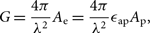 \begin{equation} G = \frac{4\pi}{\lambda^2}A_{\text{e}} = \frac{4\pi}{\lambda^2}\epsilon_{\text{ap}}A_{\text{p}},\end{equation}
where  $\lambda$
is the observing wavelength.
$\lambda$
is the observing wavelength.
Another proxy for antenna gain arises from the concept of antenna temperature,  $T_{\text{a}}$
, defined as the temperature of a fictitious matched resistor which, if substituted for the antenna, would produce the same increase in power density at the input to the receiver as an unpolarized radio source of flux density S. It can be shown (e.g., Krauss Reference Krauss1966) that:
$T_{\text{a}}$
, defined as the temperature of a fictitious matched resistor which, if substituted for the antenna, would produce the same increase in power density at the input to the receiver as an unpolarized radio source of flux density S. It can be shown (e.g., Krauss Reference Krauss1966) that:
 \begin{equation} \frac{T_{\text{a}}}{S} = \frac{A_{\text{e}}}{2k},\end{equation}
where k is the Boltzmann constant. Antenna gain expressed in this form is often referred to as ‘degrees per flux unit’ (DPFU). Here we define it thus:
 \begin{equation} G_{\text{DPFU}} \equiv \frac{A_{\text{e}}}{2k},\end{equation}
to distinguish it from the dimensionless gain G while retaining some consistency with usage elsewhere (particularly in the pulsar literature) where a plain G is often used. This quantity is typically rendered in units of  $\text{K\,Jy}^{-1}$
, where the jansky (Jy) corresponds to
$\text{K\,Jy}^{-1}$
, where the jansky (Jy) corresponds to  $10^{-26}\,\text{W\,m}^{-2}\,\text{Hz}^{-1}$
. For the 64-m Parkes telescope
$10^{-26}\,\text{W\,m}^{-2}\,\text{Hz}^{-1}$
. For the 64-m Parkes telescope  $A_{p} = 3\,217\,\text{m}^2$
and so we can write:
$A_{p} = 3\,217\,\text{m}^2$
and so we can write:
 \begin{equation} \epsilon_{\text{ap}} = 0.858[\rm Jy\,K^{-1}]\frac{T_{\text{sys}}}{S_{\text{sys}}}.\end{equation}
Various other parameters relating to the antenna beam pattern can be defined. We define the main beam of the antenna as being out to the first zero and the main beam efficiency as:
 \begin{equation} \epsilon_B \equiv \frac{\Omega_{MB}}{\Omega_A},\end{equation}
where the main beam solid angle,  $\Omega_{\text{MB}}$
, and the beam solid angle,
$\Omega_{\text{MB}}$
, and the beam solid angle,  $\Omega_A$
:
$\Omega_A$
:
 \begin{equation} \Omega_{\text{MB, A}} \equiv \frac{1}{G_{0}}\int_{\text{MB, A}} G(\theta,\phi) d\Omega,\end{equation}
(giving  $\Omega_A = 4\pi/G_{\text{0}}$
). Here
$\Omega_A = 4\pi/G_{\text{0}}$
). Here  $G_{\text{0}}$
is the peak gain of the antenna. We have presented estimates of the main beam efficiency for the UWL system as a function of frequency in Table 1.
$G_{\text{0}}$
is the peak gain of the antenna. We have presented estimates of the main beam efficiency for the UWL system as a function of frequency in Table 1.
The wideband nature of the receiver system makes it difficult to estimate the signal to noise (S/N) of a pulsar observation because the pulsar’s flux density, its pulse width, the system temperature, and telescope gain all vary with frequency. The narrowband spectral line sensitivity can be estimated using:
 \begin{equation} \sigma_s = \frac{T_{\text{sys}}}{G_{\text{DPFU}}\sqrt{n_p \tau \Delta\nu}},\end{equation}
where  $\tau$
is the total on-source integration time,
$\tau$
is the total on-source integration time,  $\Delta\nu$
is the observing bandwidth, and
$\Delta\nu$
is the observing bandwidth, and  $n_p$
is the number of recorded polarisations (1 or 2).
$n_p$
is the number of recorded polarisations (1 or 2).
Appendix B. Data collection
A publicly downloadable data collection is available from https://doi.org/10.25919/5ce76bf409bcf. This data collection contains a ‘README’ file describing the contents of the data collection and directories that contain data sets relating to beam shapes (measured and simulated), antenna and beam efficiencies, the temperature determinations presented in Figure 4 and the system equivalent flux densities shown in Figure 7. We also provide flux and polarisation calibration data files and the data files corresponding to the astronomy examples (as shown in Figures 9 and 10).
Appendix C. Author contributions
The author list has an initial non-alphabetical section giving the names of people who have led specific aspects of the project.
The remaining author list is in alphabetical order and includes the authors involved in building, installing, and commissioning the receiver system. EC, TE, VM, SO, TR, and JS were part of the commissioning team. BI provided input on the RFI sections of the paper. MB, RB, JH, MK, AM, ED, NW, LW, and WvS wrote the original funding grants. WvS updated the MEM software and contributed to polarisation and flux calibration data analysis.


