


1. Introduction
Option pricing has been a focus of mathematical research in finance since the publication of the Black–Scholes formula [Reference Black and Scholes4]. It is often considered a kind of financial derivative with the underlying stock transacting in a perfectly liquid market. However, it is widely acknowledged that not all securities are perfectly liquid. Many prior studies have provided evidence that investors ask for illiquidity premiums due to liquidity risk (see, e.g., [Reference Amihud1,Reference Amihud and Mendelson2,Reference Pástor and Stambaugh26]). Brunetti and Caldarera [Reference Brunetti and Caldarera6] built a theoretical model that studied the effects of aggregate liquidity/illiquidity on asset return volatility and correlations. Cetin et al. [Reference Cetin, Jarrow, Protter and Warachka7] considered option pricing in an extended Black–Scholes economy in which the underlying asset was not perfectly liquid. In Feng et al. [Reference Feng, Hung and Wang10], the specification of Brunetti and Caldarera [Reference Brunetti and Caldarera6] was extended to develop a new option pricing model with stochastic market liquidity. Leippold and Schärer [Reference Leippold and Schärer19] extended the discrete-time constant liquidity model of Madan [Reference Madan22], and their model successfully replicated the term and skew structures of bid-ask spreads observed in option markets. Referring to Feng et al. [Reference Feng, Hung and Wang10], Pasricha et al. [Reference Pasricha, Zhu and He25] considered all the possible correlations among the process of stock price, the mean-reversion process of liquidity risk and the process of the liquidity discount factor.
In recent decades, concerns about financial derivatives subject to default risk in the over-the-counter (OTC) markets have grown rapidly since the mid-2007, when the financial crisis erupted. Because there is no trading mechanism to guarantee the promised payment, the option holders are vulnerable to default risk, and these options with default risk are called vulnerable options. Johnson and Stulz [Reference Johnson and Stulz15] was the first to study vulnerable options by incorporating default risk into the option pricing model. In Hull and White [Reference Hull and White13], both the probability of default and the size of the proportional recovery from the default were set to be random and the authors showed that model parameters could be informed by data on bonds issued by the counterparty. Jarrow and Turnbull [Reference Jarrow and Turnbull14] considered two types of credit risks induced from the underlying assets and the writers of these derivatives. Klein [Reference Klein16] then moved forward to price vulnerable options with correlated default risk in the classical Black–Scholes model and extended the focus on stochastic default barriers in Klein and Inglis [Reference Klein and Inglis17]. Additionally, many other studies have modified the classical Black–Scholes model and worked under stochastic volatility models [Reference Lee, Yang and Kim18,Reference Wang, Wang and Zhou30,Reference Yang, Lee and Kim32]. The pricing of vulnerable options was also investigated in the jump-diffusion model and/or stochastic interest rate environment [Reference Ma, Shrestha and Xu20,Reference Ma, Yue, Wu and Ma21,Reference Niu and Wang24,Reference Tian, Wang, Wang and Wang28]. Wang et al. [Reference Wang, Wang and Shao31] presented a model with risky collateral under the assumption that holders of vulnerable options could recover a proportion of the option value using the collateral account when default occurred. Additionally, because most of the assets of financial institutions are financial assets, there exists a certain relationship between liquidity risk and default risk (see, e.g., [Reference Wang29]). He and Xiong [Reference He and Xiong11] found that deterioration of debt market liquidity leads to not only an increase in the liquidity premium of corporate bonds but also credit risk. Brogaard et al. [Reference Brogaard, Li and Xia5] focused on U.S. firms and found a negative effect of stock liquidity on default risk, suggesting that the informational efficiency of stock prices and corporate governance should be improved to enhance market liquidity and, thus, to control the level of default risk. Nadarajah et al. [Reference Nadarajah, Duong, Ali, Liu and Huang23] further confirmed this negative effect between market liquidity and default risk on a larger scale by using a sample of 46,949 firm-year observations for 4,043 nonfinancial firms across 46 countries during the 2004–2018 period.
Motivated by the empirical results mentioned above, in this paper, we mainly focus on the pricing of vulnerable European options with market liquidity risk. To model the dynamics of the imperfectly liquid underlying asset, we extend the specification in Brunetti and Caldarera [Reference Brunetti and Caldarera6] and Feng et al. [Reference Feng, Hung and Wang10]. More specifically, in our model, the stock price, the market liquidity and the liquidity discount factor are all correlated with each other and this assumption is closer to reality. Furthermore, we take the dynamic relationship between liquidity and credit risk into consideration. Default risk is described by a reduced-form model where the default intensity process is affected by the market liquidity measure. Then by utilizing the characteristic function approach and the Feynman–Kac theorem, we obtain a semi-closed form for the prices of vulnerable European options with market liquidity risk. Finally, numerical examples are presented to illustrate the effects of both liquidity risk and default risk on option prices.
The remainder of this paper is organized as follows. In Section 2, the theoretical framework is introduced. In Section 3, after providing the construction of a suitable martingale measure, we price vanilla European options in the first subsection, and value vulnerable European options in the second subsection. Section 4 is devoted to numerical analysis. Finally, we draw the conclusion of the paper in Section 5. The detailed proofs are presented in the Appendix.
2. Model settings
Consider a model with a finite time horizon  $T \gt 0$, and the filtered probability space $(\Omega,{\mathcal {F}},({\mathcal {F}}_t)_{t\geq 0},P)$ models the uncertainty in the economy, where $P$ is the physical probability measure. Suppose that there are two types of assets in the market: stocks and money market accounts. Following Brunetti and Caldarera [Reference Brunetti and Caldarera6], Feng et al. [Reference Feng, Hung and Wang10] and Wang [Reference Wang29], we assume that the stocks are not perfectly liquid, and account for liquidity risk using the liquidity discount factor. The imperfectly liquid stock price is the price that makes the demand for the stock clear its supply, and the liquidity discount factor is introduced in the demand function. Specifically, the demand for the stock depends on three factors: the stock-specific information $I_t$, the liquidity discount factor $\gamma _t$ and the stock price $S_t$. The demand function, $D(S_t,\gamma _t,I_t)$, is given by
 \begin{equation} D(S_t,\gamma_t,I_t)=g\left(\frac{I_t^\nu}{\gamma_t S_t}\right), \end{equation}
where  $g(\cdot )$ is a smooth, strictly increasing function, and $\nu$ is a positive constant.
Brunetti and Caldarera [Reference Brunetti and Caldarera6] proposed the following form of the liquidity discount factor  $\gamma _t$,
 \begin{equation} \gamma_t=\exp\left(-\beta\left(\int_0^t L_s\,{\mathrm{d}} s+\int_0^t L_s\,{\mathrm{d}} W_s^\gamma\right)\right), \quad t\geq0, \end{equation}
where  $\{W_t^\gamma \}_{t\geq 0}$ is a standard Brownian motion under $P$,
$P$,  $L_t$ is a market liquidity measure and $\beta$ is a nonnegative constant representing the sensitivity of the stock to market illiquidity.
Suppose the supply for the stock is fixed and equals  $\bar S$, and then the market clearing condition yields the expression of the imperfectly liquid stock price $S_t$ as follows,
 \begin{equation} S_t=\frac{1}{\gamma_t}\left(\frac{I_t^\nu}{g^{{-}1}(\bar S)}\right),\quad t\geq0. \end{equation}
Specially, when the liquidity discount factor  $\gamma _t\equiv 1$, the stock price (2.3) degenerates to
 \begin{equation} S_t^L=\frac{I_t^\nu}{g^{{-}1}(\bar S)}, \quad t\geq0. \end{equation}
Obviously, the price of the underlying stock affected by market liquidity can be formulated by
 \begin{equation} S_t=\frac{1}{\gamma_t}S_t^L, \quad t\geq0. \end{equation}
As we know, liquidity risk is a financial risk that for a certain period of time a given financial asset, security or commodity cannot be traded quickly enough in the market without impacting the market price. Liquidity risk usually arises from situations in which a party interested in trading an asset cannot do it because nobody in the market wants to trade for that asset. Hence, risk-averse investors naturally require higher expected return as compensation for liquidity risk. In order to understand the effect of liquidity risk more clearly, we now consider a special case of (2.5) when  $L_t$ is deterministic and the liquidity discount factor is independent of $S_t^L$. In this special case, from (2.2) and (2.5), we have the following conditional expectation,
 \begin{align} E^P[S_t\,|\,S_t^L]& =E^P\left[\exp\left(\beta\left(\int_0^t L_s\,{\mathrm{d}} s+\int_0^t L_s\,{\mathrm{d}} W_s^\gamma\right)\right)S_t^L\,|\,S_t^L\right]\nonumber\\ & =S_t^L\exp\left(\int_0^t\left(\beta L_s +\frac{1}{2}\beta^2 L_s^2\right){\mathrm{d}} s\right). \end{align}
When  $\beta L_t$ is small, the integral in (2.6) will have the same sign as its first term, and hence, $\exp (\int _0^t(\beta L_s + \frac {1}{2}\beta ^2 L_s^2)\,{\mathrm {d}} s)$ can be interpreted as a convenience yield caused by the illiquidity. Therefore, the value of $L_t$ can be interpreted as the level of market liquidity at time $t$, and $L_t=0$ means that the market liquidity is at the perfect level. Additionally, $L_t \gt 0$ corresponds to shortages, while $L_t \lt 0$ corresponds to gluts (see, e.g., [Reference Brunetti and Caldarera6]).
In what follows, we focus on the dynamics of the market liquidity measure  $L_t$ and the liquidity discount factor $\gamma _t$. Using S $\& $P 500 index data, Feng et al. [Reference Feng, Hung and Wang10] found that market liquidity tends to fluctuate around the mean, which means that $L_t$ has the mean-reverting property, so we model it as
 \begin{equation} {\mathrm{d}} L_t=\kappa_L(\theta_L-L_t)\,{\mathrm{d}} t+\sigma_L\,{\mathrm{d}} W_t^L, \quad t\geq0, \end{equation}
where  $\{W_t^L\}_{t\geq 0}$ is also a standard Brownian motion under $P$;
$P$;  $\kappa _L$ is the mean-reversion speed of market liquidity; $\theta _L$ is the mean level and $\sigma _L$ is the volatility. According to Itô's lemma, the liquidity discount factor $\gamma _t$ in (2.2) can be written in the following form:
 \begin{equation} \frac{{\mathrm{d}} \gamma_t}{\gamma_t}=\left(-\beta L_t+\frac{1}{2}\beta^2L_t^2\right){\mathrm{d}} t-\beta L_t\,{\mathrm{d}} W_t^\gamma, \quad t\geq0, \ \gamma_0=1. \end{equation}
Next, we turn to the dynamics of  $S_t^L$, and then using (2.5), we can obtain the time- $t$ price $S_t$ of the imperfectly liquid stock. Note that under the assumptions of the fixed supply for the stock and the form of the specific demand function, Brunetti and Caldarera [Reference Brunetti and Caldarera6] proved that $S_t^L$ is a geometric Brownian motion which is consistent with the classical Black–Scholes model. Here, we also adopt the classical B-S model,
 \begin{equation} \frac{{\mathrm{d}} S_t^L}{S_t^L}=\mu_S\,{\mathrm{d}} t+\sigma_S\,{\mathrm{d}} W_t^S, \quad t\geq0, \end{equation}
where  $\mu _S,\sigma _S$ are positive constants and $\{W_t^S\}_{t\geq 0}$ is a standard Brownian motion under $P$.
$P$.
In this paper, we work in a more general framework by assuming that  $W_t^S$, $W_t^\gamma$ and $W_t^L$ are correlated with each other. Moreover, their correlation structure is listed below:
 \begin{equation} \begin{aligned} \langle {\mathrm{d}} W_t^S,{\mathrm{d}} W_t^\gamma\rangle & =\rho_1\,{\mathrm{d}} t,\\ \langle {\mathrm{d}} W_t^S,{\mathrm{d}} W_t^L\rangle & =\rho_2\,{\mathrm{d}} t,\\ \langle {\mathrm{d}} W_t^L,{\mathrm{d}} W_t^\gamma\rangle & =\rho_3\,{\mathrm{d}} t. \end{aligned} \end{equation}
Now from (2.5), (2.8) and (2.9), Itô's lemma implies that the time- $t$ price $S_t$ of the imperfectly liquid stock is given by the following process:
 \begin{equation} \frac{{\mathrm{d}} S_t}{S_t}=\left(\mu_S+\beta L_t+\frac{1}{2}\beta^2L^2_t+\rho_1\sigma_S\beta L_t\right){\mathrm{d}} t+\sigma_S\,{\mathrm{d}} W_t^S+\beta L_t \,{\mathrm{d}} W_t^\gamma. \end{equation}
From the above equation, it is easy to see that market liquidity measure  $L_t$ affects the return and the volatility of the stock simultaneously under the physical probability measure $P$.
$P$.
3. Options pricing
This section presents the procedures to derive the prices of vanilla European options and vulnerable European options when the underlying assets are not perfectly liquid.
3.1. Pricing of vanilla European options with liquidity risk
To price options, we need to determine an equivalent martingale measure. Bingham and Kiesel [Reference Bingham and Kiesel3] illustrated that all possible martingale measures could be characterized by their Girsanov identities. Here, we select a suitable equivalent martingale measure using the following Radon–Nikodym derivative:
 \begin{equation} \left.\frac{{\mathrm{d}} Q}{{\mathrm{d}} P}\right|_{{\mathcal{F}}_t}= \exp\left\{-\int_0^t\lambda^S_s\,{\mathrm{d}} W^S_s -\int_0^t\lambda^\gamma_s\,{\mathrm{d}} W^{\gamma}_s-\frac{1}{2}\int_0^t(\lambda^S_s)^2\,{\mathrm{d}} s -\frac{1}{2}\int_0^t(\lambda^\gamma_s)^2\,{\mathrm{d}} s-\rho_1\int_0^t\lambda^S_s\lambda^\gamma_s\,{\mathrm{d}} s\right\}, \end{equation}
where  $\lambda ^S_t$ and $\lambda ^\gamma _t$ satisfy
 \begin{equation} \lambda^S_t(\rho_1\beta L_t+\sigma_S)+\lambda^\gamma_t(\beta L_t+\rho_1\sigma_S)=\mu_S+\beta L_t+\tfrac{1}{2}\beta^2L_t^2+\rho_1\sigma_S\beta L_t-r, \end{equation}
with  $r$ being a constant risk-free interest rate. Using Girsanov's theorem, the three-dimensional process $\{W^Q_t=(W_t^{Q,L},\ W_t^{Q,\gamma },\ W_t^{Q,S});\ 0\leq t \lt \infty \}$ defined by
 \begin{equation} \begin{aligned} {\mathrm{d}} W_t^{Q,L} & = {\mathrm{d}} W_t^{L}+\rho_2\lambda^S_t\,{\mathrm{d}} t+\rho_3\lambda^\gamma_t\,{\mathrm{d}} t,\\ {\mathrm{d}} W_t^{Q,\gamma} & = {\mathrm{d}} W_t^{\gamma}+\lambda^\gamma_t\,{\mathrm{d}} t+\rho_1\lambda^S_t\,{\mathrm{d}} t,\\ {\mathrm{d}} W_t^{Q,S} & = {\mathrm{d}} W_t^{S}+\lambda^S_t\,{\mathrm{d}} t+\rho_2\lambda^\gamma_t\,{\mathrm{d}} t, \end{aligned} \end{equation}
is a standard Brownian motion under  $Q$, and it has the same correlation structure as that under the physical probability measure $P$. Furthermore, the stock price dynamics under $Q$ can be written as
 \begin{equation} \frac{{\mathrm{d}} S_t}{S_t}=r\,{\mathrm{d}} t+\beta L_t\,{\mathrm{d}} W_t^{Q,\gamma}+\sigma_S\,{\mathrm{d}} W_t^{Q,S}, \end{equation}
with
 \begin{equation} {\mathrm{d}} L_t=(\kappa_L\theta_L-\kappa_L L_t-\sigma_L\rho_2\lambda^S_t-\sigma_L\rho_3\lambda^\gamma_t)\,{\mathrm{d}} t +\sigma_L\,{\mathrm{d}} W^{Q,L}_t. \end{equation}
According to the expression of  ${\mathrm {d}} W_t^{Q,L}$ in (3.3), the market liquidity risk premium is $\rho _2\lambda ^S_t+\rho _3\lambda ^\gamma _t$. Following the idea of Heston [Reference Heston12] as the means of achieving tractability, we assume that the liquidity risk premium is proportional to the level of market liquidity, that is,
 \begin{equation} \rho_2\lambda^S_t+\rho_3\lambda^\gamma_t=\frac{\xi L_t}{\sigma_L}, \end{equation}
where  $\xi$ is a constant. In other words, the measure change adjusts the drift of the market liquidity measure $L_t$ by the term ${\xi L_t}/{\sigma _L}$ (also see [Reference Feng, Hung and Wang10]). Thus, we can rewrite the dynamics of the market liquidity measure under $Q$,
$Q$,
 \begin{equation} {\mathrm{d}} L_t=\kappa (\theta-L_t)\,{\mathrm{d}} t+\sigma_L\,{\mathrm{d}} W_t^{Q,L}, \end{equation}
where  $\kappa := \kappa _L+\xi$ and $\theta := {\kappa _L\theta _L}/{(\kappa _L+\xi )}$.
To facilitate our analysis of the stock price, under the equivalent martingale measure  $Q$, we intend to rewrite Brownian motion $W^Q_t=(W_t^{Q,L},W_t^{Q,\gamma },W_t^{Q,S})$ as a linear transformation of a three-dimensional standard Brownian motion. First, denote the correlation matrix of $W^Q_t$ by $\Lambda$, which is given by
 $$\Lambda = \left(\begin{array}{ccc} 1 & \rho_3 & \rho_2\\ \rho_3 & 1 & \rho_1\\ \rho_2 & \rho_1 & 1\\ \end{array}\right).$$
Applying the Cholesky decomposition, we can decompose  $\Lambda$ into the product of a lower triangular matrix $A$ and its conjugate transpose, where
 $$A = \left(\begin{array}{ccc} 1 & 0 & 0\\ \rho_3 & \sqrt{1-\rho_3^2} & 0\\ \rho_2 & \zeta & \sqrt{1-\rho_2^2-\zeta^2}\\ \end{array}\right),$$
and  $\zeta ={(\rho _1-\rho _2\rho _3)}/{\sqrt {1-\rho _3^2}}$. Then, one obtains that
 \begin{equation} \begin{aligned} W_t^{Q,L} & =W^Q_{1,t},\\ W_t^{Q,\gamma} & =\rho_3W^Q_{1,t}+\sqrt{1-\rho_3^2}W^Q_{2,t},\\ W_t^{Q,S} & =\rho_2W^Q_{1,t}+\zeta W^Q_{2,t}+\sqrt{1-\rho_2^2-\zeta^2}W^Q_{3,t}, \end{aligned} \end{equation}
and  $W^Q_{1,t}$, $W^Q_{2,t}$ and $W^Q_{3,t}$ are independent standard Brownian motions under $Q$. Therefore, the stock price can be rewritten as:
 \begin{align} \frac{{\mathrm{d}} S_t}{S_t}& =r\,{\mathrm{d}} t+(\rho_2\sigma_S+\rho_3\beta L_t)\,{\mathrm{d}} W^Q_{1,t}\nonumber\\ & \quad +(\zeta\sigma_S+\sqrt{1-\rho_3^2}\beta L_t)\,{\mathrm{d}} W^Q_{2,t}+\sqrt{1-\rho_2^2-\zeta^2}\sigma_S\,{\mathrm{d}} W^Q_{3,t}, \end{align}
with the market liquidity measure  $L_t$ given below,
 \begin{equation} {\mathrm{d}} L_t=\kappa(\theta-L_t)\,{\mathrm{d}} t+\sigma_L\,{\mathrm{d}} W^Q_{1,t}. \end{equation}
Obviously,  $\{S_t, t\geq 0\}$ is a martingale after discounted by the risk-free cash account under $Q$.
$Q$.
Now, we are ready to derive the price of vanilla European options. At time  $t=0$, the price of a European call option with maturity $T$ and strike price $K$ is given by
 \begin{align} C_0& =e^{{-}r T}E^Q[\max(S_T-K,0)]\nonumber\\ & = e^{{-}rT}E^Q[(S_T-K)I_{\{S_T \gt K\}}]\nonumber\\ & = e^{{-}r T}E^Q[S_T I_{\{\ln S_T \gt \ln K\}}]-Ke^{{-}r T} Q(\ln S_T \gt \ln K), \end{align}
where  $I_{\{\cdot \}}$ is the indicator function. To calculate $C_0$, we use the characteristic function of $\ln (S_T)$ defined by $f_1(\phi ):=E^Q[e^{\phi \ln S_T}]$ for any complex number $\phi$. Using the Fourier inversion formula and following [Reference Shephard27], we can obtain the explicit expressions of the two components in (3.11) as follows:
 \begin{align} I_1& :=E^Q[S_T I_{\{\ln S_T \gt \ln K\}}]\nonumber\\ & =\frac{1}{2}f_1(1)+\frac{1}{\pi}\int_0^\infty\textrm{Re} \left[\frac{K^{{-}i\phi}f_1(i\phi+1)}{i\phi}\right]{\mathrm{d}}\phi, \end{align}
and
 \begin{align} I_2& := Q(\ln S_T \gt \ln K)\nonumber\\ & =\frac{1}{2}+\frac{1}{\pi}\int_0^\infty\textrm{Re}\left[\frac{K^{{-}i\phi}f_1(i\phi)}{i\phi}\right]{\mathrm{d}}\phi. \end{align}
Additionally, the explicit expression of the characteristic function  $f_1(\phi ):=E^Q[e^{\phi \ln S_T}]$ will be given as a special case in the following subsection.
3.2. Pricing of vulnerable European options with liquidity risk
In this subsection, we incorporate default risk of option issuers into the pricing model. Here, we describe default risk in a reduced-form model, and work under the equivalent martingale measure  $Q$ directly for valuation purposes.Footnote 1 Assume that the underlying asset price is driven by (3.9), and let $\tau$ be the default time modeled by the first jump time of a doubly stochastic Poisson process with the following intensity process:
 \begin{equation} \lambda_t=\eta_0+ \eta_1 L_t+ \eta_2 L_t^2+ X_t. \end{equation}
And  $X_t$ is captured by a mean-reverting square root process,
 \begin{equation} {\mathrm{d}} X_t=(\gamma_X-\alpha_X X_t)\,{\mathrm{d}} t+\sigma_X\sqrt{X_t}\,{\mathrm{d}} B^Q_t, \end{equation}
with  $X_0 \gt 0$ and $B^Q_t$ being a standard Brownian motion under $Q$, independent of $W_{1,t}^Q$, $W_{2,t}^Q$ and $W_{3,t}^{Q}$. To ensure that $\lambda _t$ is nonnegative, we need to pose the assumptions on the parameters that $\eta _2 \gt 0$ and $4\eta _0\eta _2\geq \eta _1^2$. There are two remarks on the assumption of the intensity process. First, the default intensity (3.14) consists of two parts: market liquidity $L_t$ and idiosyncratic risk $X_t$, and market liquidity is a common factor to default intensity processes and all stocks in the market. Second, we propose a general form of the intensity process, which could also allow us to achieve tractability. Specially, with $\eta _1=0$, the model could capture negative effects between market liquidity ( $|L_t|$) and default risk ( $\lambda _t$). We refer interested readers to Brogaard et al. [Reference Brogaard, Li and Xia5] and Nadarajah et al. [Reference Nadarajah, Duong, Ali, Liu and Huang23] for this negative effect.
Now we are ready to price vulnerable European options. Let  $\bar {\alpha }$ be the recovery rate, and then the vulnerable option price is given by
 \begin{equation} D_0=e^{{-}rT}E^Q[I_{\{\tau \gt T\}}(S_T-K)^+]+\bar{\alpha} e^{{-}rT}E^Q[I_{\{0 \lt \tau\leq T\}}(S_T-K)^+]. \end{equation}
In the proposed pricing model, we can derive the semi-closed form of the vulnerable option price  $D_0$. To this end, we define the Fourier transform of $(\ln (S_T),\int _0^T \lambda _s\,{\mathrm {d}} s)$, denoted by $f(\phi,\psi )$,
 \begin{equation} f(\phi,\psi)=E^Q[e^{\phi\ln S_T +\psi\int_0^T \lambda_s\,{\mathrm{d}} s}], \end{equation}
where  $\phi$ and $\psi$ are complex numbers. Because $\{X_t, t\geq 0\}$ is independent of the other processes, we obtain that
 \begin{align} f(\phi,\psi)& =E^Q[e^{\phi\ln S_T +\psi\int_0^T (\eta_0+ \eta_1 L_s+ \eta_2 L_s^2)\,{\mathrm{d}} s}]\times E^Q[e^{\psi\int_0^T X_s\,{\mathrm{d}} s}]\nonumber\\ & :=f_{SL}(\phi,\psi)\times f_X(\psi), \end{align}
where  $f_{SL}(\phi,\psi )=E^Q[e^{\phi \ln S_T +\psi \int _0^T (\eta _0+ \eta _1 L_s+ \eta _2 L_s^2)\,{\mathrm {d}} s}]$ and $f_X(\psi )=E^Q[e^{\psi \int _0^T X_s\,{\mathrm {d}} s}]$. In addition, the closed-form expressions of $f_X(\psi )$ and $f_{SL}(\phi,\psi )$ are shown in the following proposition.
Proposition 3.1. Let  $\mu _1(\psi )=\sqrt {\alpha _X^2-2\psi \sigma _X^2}$ and $\mu _2(\psi )={(\alpha _X+\mu _1(\psi ))}/{(\alpha _X-\mu _1(\psi ))}$. The closed-form expressions of $f_X(\psi )$ and $f_{SL}(\phi,\psi )$ are given by
 \begin{align} f_X(\psi) & =\exp\left\{\frac{(\alpha_X+\mu_1(\psi))(1-e^{\mu_1(\psi)T})}{\sigma_X^2(1-\mu_2(\psi) e^{\mu_1(\psi)T})}X_0\right.\nonumber\\ & \quad \left.+\frac{\mu_1(\psi)}{\sigma_X^2}\left((\alpha_X+\mu_1(\psi))T -2\ln\left(\frac{1-\mu_2(\psi) e^{\mu_1(\psi)T}}{1-\mu_2(\psi)}\right)\right)\right\}, \end{align}
and
 \begin{equation} f_{SL}(\phi,\psi)=\exp\{\phi Y_0+\tfrac{1}{2}A_1(0,T)L_0^2+A_2(0,T)L_0+A_3(0,T)\}, \end{equation}
where
 $$Y_0=\ln S_0+\left(r-\frac{1}{2}\sigma_S^2-\frac{\tilde{\kappa}\tilde{\theta}\rho_2\sigma_S} {\sigma_L}-\frac{\sigma_L\rho_3\beta}{2}+\frac{1}{2}\phi\sigma_S^2(1-\rho_2^2)+\frac{\psi\eta_0}{\phi}\right)T-\frac{\rho_3\beta}{2 \sigma_L}L_0^2-\frac{\rho_2\sigma_S}{\sigma_L}L_0,$$
and  $A_1(0,T)$, $A_2(0,T)$ and $A_3(0,T)$ are given by (A.10)–(A.12) in the Appendix.
Proof. See the Appendix.
Note that when  $\psi =0$, $f(\phi,0)$ is the characteristic function of $\ln (S_T)$, that is, $f(\phi,0)=f_1(\phi ):=E^Q[e^{\phi \ln S_T}]$. Using the Fourier inversion formula and the characteristic functions, we can derive the price of vulnerable options and the results are given in the following proposition.
Proposition 3.2. Under the risk-neutral martingale measure  $Q$, the time- $t$ price of vulnerable European call options with liquidity risk can be calculated as follows:
 \begin{equation} D_0 =(1-\bar{\alpha})e^{{-}rT}(I_3-KI_4)+\bar{\alpha} C_0, \end{equation}
where  $C_0$ is given in (3.11), and
 \begin{align} I_3& =\frac{1}{2}f(1,-1)+\frac{1}{\pi}\int_{0}^\infty\textrm{Re}\left[\frac{K^{{-}i\phi}f(i\phi+1,-1)}{ i\phi }\right]{\mathrm{d}}\phi, \end{align}
 \begin{align} I_4& =\frac{1}{2}f(0,-1)+\frac{1}{\pi}\int_{0}^\infty \textrm{Re}\left[\frac{K^{{-}i\phi}f(i\phi,-1)}{ i\phi }\right]{\mathrm{d}} \phi. \end{align}
Proof. It can be easily seen that  $D_0$ in (3.16) can be rewritten as
 $$D_0 =(1-\bar{\alpha})e^{{-}rT}(I_3-KI_4)+\bar{\alpha} C_0,$$
where  $C_0$ is the price of vanilla European options with liquidity risk given in (3.11), and
 \begin{align*} I_3& :=E^Q[S_TI_{\{\tau \gt T,\ S_T\geq K\}}],\\ I_4& :=E^Q[I_{\{\tau \gt T,\ S_T\geq K\}}]. \end{align*}
Employing the inverse Fourier transform, we can obtain the following expressions of  $I_3$ and $I_4$:
 \begin{align*} I_3& =\frac{1}{2}f(1,-1)+\frac{1}{\pi}\int_{0}^\infty\textrm{Re}\left[\frac{K^{{-}i\phi}f(i\phi+1,-1)}{ i\phi }\right]{\mathrm{d}}\phi,\\ I_4& =\frac{1}{2}f(0,-1)+\frac{1}{\pi}\int_{0}^\infty \textrm{Re}\left[\frac{K^{{-}i\phi}f(i\phi,-1)}{ i\phi }\right]{\mathrm{d}} \phi. \end{align*}
This completes the proof of Proposition 3.2.
4. Numerical analysis
In this section, we illustrate the effect of market liquidity risk on the prices of (vulnerable) European options. To show the results explicitly, we mainly illustrate prices of call options in three situations: the proposed framework with both liquidity risk and default risk, the case without liquidity risk (i.e.,  $\beta =0$), and the case without default risk (i.e., $\bar {\alpha }=1$).
Following Pasricha et al. [Reference Pasricha, Zhu and He25], we use the following parameter values:  $\sigma _S=0.2$, $\sigma _L=0.9$, $\rho _1=0.25$, $\rho _2=0.35$, $\rho _3=0$, $\tilde {\kappa }=0.3$, $\tilde {\theta }=0.2$ and $\beta =0.5$. Theoretically, the less liquidity the financial market holds, the more likely option issuers are to default. As a result, the assumption that the parameters in (3.14) are positive is reasonable. We find that when setting $\eta _0=0.02$, $\eta _1=0.02$ and $\eta _2=0.02$, the default probability in 2 years is approximately $7.34\%$. Additionally, $\bar {\alpha }=0.6$ means that 60% of the loss can be recovered after default, which is a conservative value. Without loss of generality, we set the interest rate $r=0.01$, $S_0=100$, $L_0=0.3$, and the option is at the money ( $S_0=K=100$) with a maturity of $2.0$ years.
First, we focus on the effect of stochastic liquidity risk on the prices of both vanilla and vulnerable call options. From Figure 1, we can intuitively find that call option prices decrease with higher strike prices. To go further, it can also be found that by comparing the distance between the two lines, both the liquidity risk and default risk have small effects on in-the-money options. In contrast, with the augmentation of strike prices, the impact of liquidity risk always remains pronounced, while the impact of default risk becomes relatively more negligible, and these observations are consistent with Wang [Reference Wang29]. The large price discrepancies suggest that when pricing options, option issuers should take market liquidity into consideration. In addition, option buyers should be clear about the credit status of each issuer with the help of credit rating agencies or other possible channels and only accept reasonable prices that include default risk premiums.

Figure 1. Call option prices against strike prices. The solid, dashed and dotted lines correspond to prices in the proposed framework, prices without liquidity risk ( $\beta =0$) and prices without default risk ( $\bar {\alpha }=1$), respectively.
Figure 2 displays the relationship between call option prices and the values of the sensitivity level of the stock to market illiquidity. Undoubtedly, option prices in the pricing model without liquidity risk are not affected by the changes of  $\beta$, hence, we obtain a constant number in this case. Regarding the other two cases, call option prices rise when the stock becomes more sensitive to market illiquidity. Comparing the distance between two lines, the effect of default risk on the prices becomes relatively evident with a larger $\beta$. It should be noted that the values of $\beta$ affect the total volatility of the underlying stock.
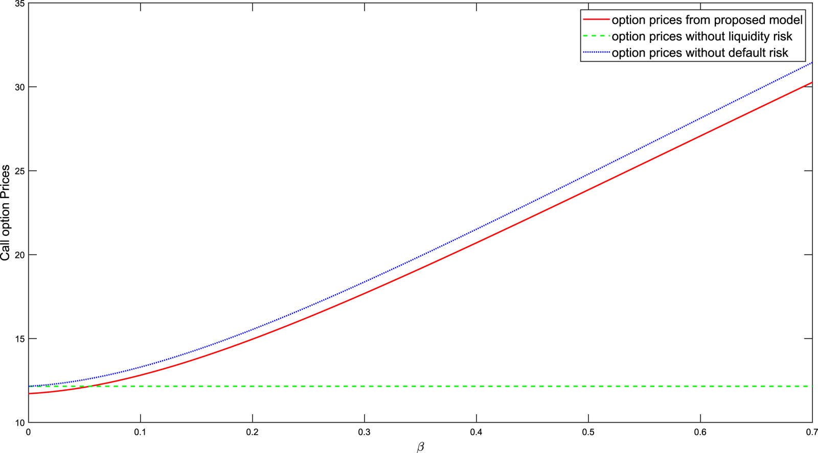
Figure 2. Call option prices against the values of the sensitivity level of the stock to the market illiquidity. The solid, dashed and dotted lines correspond to prices in the proposed framework, prices without liquidity risk ( $\beta =0$) and prices without default risk ( $\bar {\alpha }=1$), respectively.
Figure 3 illustrates call option prices with different volatilities of the underlying stock. A higher volatility corresponds to a higher option price. We can observe two different trends from this graph: with an increasing volatility of the underlying stock, the dotted line and the solid line tend to be farther away from each other, while the solid line and the dashed line get closer to each other, showing the strengthening effect of default risk and the weakening impact of liquidity risk. This is because the instantaneous total variance of the underlying stock is  $\sigma ^2_S+\beta ^2 L^2_t+2\rho _1\sigma _S\beta L_t$, and the effect of liquidity risk is not so significant with a bigger $\sigma _S$. We need to mention that in the real world, the probability of stock prices fluctuating fiercely in a short period is relatively low. As a result, we shall focus more on call option prices with smaller $\sigma _S$, and pay more attention to the influence of the stochastic liquidity risk.

Figure 3. Call option prices against volatilities of the underlying stock. The solid, dashed and dotted lines correspond to prices in the proposed framework, prices without liquidity risk ( $\beta =0$) and prices without default risk ( $\bar {\alpha }=1$), respectively.
Figure 4 depicts call option prices with different volatilities of market liquidity risk itself. Evidently, we obtain a horizontal line without liquidity risk. In regard to the dotted line and the solid one, a larger  $\sigma _L$ induces a correspondingly higher option price. Observing the differences between the solid and dashed lines, we find that the effect of liquidity risk is enhanced as the values of $\sigma _L$ rise. Based on the bid-ask spread, market liquidity can be captured even though it is an invisible variable (see, e.g., [Reference Amihud1,Reference Corwin and Schultz8]). Therefore, investors could easily estimate the value of $\sigma _L$ and eventually trade options around a reasonable price using the model developed in this paper.

Figure 4. Call option prices against volatilities of the stock market liquidity. The solid, dashed and dotted lines correspond to prices in the proposed framework, prices without liquidity risk ( $\beta =0$) and prices without default risk ( $\bar {\alpha }=1$), respectively.
Figure 5 illustrates call option prices with respect to the correlation coefficients between the liquidity measure  $L_t$ and the liquidity discount factor $\gamma _t$. When $\rho _3$ is negative, call option prices increase with the correlation coefficients approaching to zero. In contrast, in the case of $\rho _3 \gt 0$, the marginal rise of call option prices decreases and even becomes negative when $\rho _3$ is large enough. In addition, the effect of default risk on option prices is much more pronounced when $\rho _3$ takes a larger value.

Figure 5. Call option prices against  $\rho _3$. The solid and dotted lines correspond to prices in the proposed framework and prices without default risk ( $\bar {\alpha }=1$), respectively.
Figure 6 shows call option prices against  $\eta _1$, displaying a U-shaped curve in the proposed model. $\eta _1$ is the coefficient of the first-order term in the intensity process $\lambda _t$. Call option prices first decrease and then increase as $\eta _1$ increases. Comparing the distance between two lines, we can easily find that the effect of default risk is evident when $\eta _1$ is small and the effect reaches the maximum under a certain $\eta _1$. This is because the corresponding default probabilities first increase and then decrease as shown in Figure 8. Figure 7 shows call option prices with respect to $\eta _2$. $\eta _2$ is the coefficient of the second-order term in the intensity process $\lambda _t$. Since $L^2_t$ is always positive, default probabilities increase and then vulnerable call option prices drop with an increase of $\eta _2$, which can also be verified in Figure 9.

Figure 6. Call option prices against  $\eta _1$. The solid and dotted lines correspond to prices in the proposed framework and prices without default risk ( $\bar {\alpha }=1$), respectively.

Figure 7. Call option prices against  $\eta _2$. The solid and dotted lines correspond to prices in the proposed framework and prices without default risk ( $\bar {\alpha }=1$), respectively.

Figure 8. Default probabilities against  $\eta _1$. The solid line corresponds to default probabilities in the proposed framework.

Figure 9. Default probabilities against  $\eta _2$. The solid line corresponds to default probabilities in the proposed framework.
5. Conclusion
In this paper, we contribute to the literature on vulnerable European options by taking the possibility of default risk caused by the counterparty and market liquidity risk into consideration. A general correlation structure among the underlying asset, the liquidity discount factor and the default intensity process is specified. Utilizing the characteristic function and the Feynman–Kac theorem, we obtain the semi-closed form pricing formulae of vulnerable European options with market liquidity risk. Finally, numerical experiments are performed to illustrate the effects of liquidity risk and default risk on the prices of vulnerable European options.
Acknowledgments
The authors would like to thank anonymous referees and editors for providing a number of valuable comments that led to several important improvements. All errors are our own responsibilities.
Competing interests
The authors declare no conflict of interest.
Appendix
Here, we derive the expressions of  $f_X(\psi )$ and $f_{SL}(\phi,\psi )$. First, using the dynamics of $X_t$ in (3.15), we can derive the expression of $f_X(\psi )$ easily,
 \begin{align} f_X(\psi)& =E^Q[e^{\psi\int_0^T X_s{\mathrm{d}} s}] =\exp\left\{\frac{(\alpha_X+\mu_1(\psi))(1-e^{\mu_1(\psi)T})} {\sigma_X^2(1-\mu_2(\psi) e^{\mu_1(\psi)T})}X_0\right.\nonumber\\ & \quad \left.+\frac{\mu_1(\psi)}{\sigma_X^2}\left((\alpha_X+\mu_1(\psi))T -2\ln\left(\frac{1-\mu_2(\psi) e^{\mu_1(\psi)T}}{1-\mu_2(\psi)}\right)\right)\right\}, \end{align}
where  $\mu _1(\psi )=\sqrt {\alpha _X^2-2\psi \sigma _X^2}$ and $\mu _2(\psi )={(\alpha _X+\mu _1(\psi ))}/{(\alpha _X-\mu _1(\psi ))}$.
Next, we turn to the calculation of  $f_{SL}(\phi,\psi )$. Note that
 \begin{align} \ln S_T& =\ln S_0+\left(r-\frac{1}{2}\sigma_S^2\right)T+\int_0^T(\rho_2\sigma_S+\rho_3\beta L_s)\,{\mathrm{d}} W_{1,s}^Q\nonumber\\ & \quad +\int_0^T(\zeta\sigma_S+\beta\sqrt{1-\rho_3^2} L_s)\,{\mathrm{d}} W_{2,s}^Q\nonumber\\ & \quad +\sigma_S\sqrt{1-\rho_2^2-\zeta^2} W_{3,T}^Q-\frac{1}{2}\beta^2\int_0^T L_s^2\,{\mathrm{d}} s-\rho_1\beta\sigma_S\int_0^T L_s\,{\mathrm{d}} s. \end{align}
From the dynamics of  $L_t$ in (2.7), we apply Itô's lemma to $L_t^2+({2\rho _2\sigma _S}/{\rho _3\beta })L_t$, and obtain the following result,
 \begin{align} {\mathrm{d}}\left(L_t^2+\frac{2\rho_2\sigma_S}{\rho_3\beta}L_t\right) & =2\left(L_t+\frac{\rho_2\sigma_S}{\rho_3\beta}\right){\mathrm{d}} L_t+\sigma^2_L\,{\mathrm{d}} t\nonumber\\ & =\left(2\tilde{\kappa}(\tilde{\theta}-L_t)\left(L_t+\frac{\rho_2\sigma_S}{\rho_3\beta}\right)+\sigma^2_L\right){\mathrm{d}} t+2 \sigma_L \left(L_t+\frac{\rho_2\sigma_S}{\rho_3\beta}\right){\mathrm{d}} W_{1,t}^Q, \end{align}
which in turn implies that
 \begin{align} \int_0^T\left(L_s+\frac{\rho_2\sigma_S}{\rho_3\beta}\right){\mathrm{d}} W_{1,s}^Q & ={-}\frac{1}{2\sigma_L}L_0^2-\frac{\rho_2\sigma_S}{\sigma_L\rho_3\beta}L_0 -\left(\frac{\tilde{\kappa}\tilde{\theta}\rho_2\sigma_S} {\sigma_L\rho_3\beta}+\frac{\sigma_L}{2}\right)T\nonumber\\ & \quad +\frac{1}{2\sigma_L}L_T^2+\frac{\rho_2\sigma_S}{\sigma_L\rho_3\beta}L_T -\frac{\tilde{\kappa}}{\sigma_L}\left(\tilde{\theta}-\frac{ \rho_2\sigma_S}{\rho_3\beta}\right)\int_0^T L_s\,{\mathrm{d}} s +\frac{\tilde{\kappa}}{\sigma_L} \int_0^T L_s^2\,{\mathrm{d}} s. \end{align}
Therefore, one can get that
 \begin{align} f_{SL}(\phi,\psi)& =E^Q[e^{\phi\ln S_T +\psi\int_0^T (\eta_0+ \eta_1 L_s+ \eta_2L_s^2)\,{\mathrm{d}} s}]\nonumber\\ & =\exp\left\{\phi\left(\ln S_0+\left(r-\frac{1}{2}\sigma_S^2\right)T\right)\right\}E^Q \left[\exp\left\{\phi\left(\int_0^T(\rho_2\sigma_S+\rho_3\beta L_s)\,{\mathrm{d}} W_{1,s}^Q\right.\right.\right.\nonumber\\ & \quad + \int_0^T(\zeta\sigma_S+\beta\sqrt{1-\rho_3^2} L_s){\mathrm{d}} W_{2,s}^Q+\sigma_S\sqrt{1-\rho_2^2-\zeta^2} W_{3,T}^Q\nonumber\\ & \quad \left.\left.\left.-\frac{1}{2}\beta^2\int_0^T L_s^2\,{\mathrm{d}} s-\rho_1\beta\sigma_S\int_0^T L_s\,{\mathrm{d}} s\right)+\psi\int_0^T (\eta_0+ \eta_1 L_s+ \eta_2 L_s^2)\,{\mathrm{d}} s\right\}\right]\nonumber\\ & =\exp\left\{\phi\left(\ln S_0+\left(r-\frac{1}{2}\sigma_S^2-\frac{\tilde{\kappa}\tilde{\theta}\rho_2\sigma_S} {\sigma_L}-\frac{\sigma_L\rho_3\beta}{2}\right)T-\frac{\rho_3\beta}{2 \sigma_L}L_0^2-\frac{\rho_2\sigma_S}{\sigma_L}L_0\right)+\psi\eta_0 T\right\}\nonumber\\ & \quad \times E^Q\left[\exp\left\{\phi\left(\frac{\rho_3\beta}{2 \sigma_L}L_T^2+\frac{\rho_2\sigma_S}{\sigma_L}L_T-\frac{\tilde{\kappa}}{\sigma_L}(\tilde{\theta}\rho_3\beta-\rho_2\sigma_S)\int_0^T L_s\,{\mathrm{d}} s+\frac{\tilde{\kappa}\rho_3\beta}{\sigma_L}\int_0^T L_s^2\,{\mathrm{d}} s\right)\right.\right.\nonumber\\ & \quad +\frac{1}{2}\phi^2\zeta^2\sigma^2_S T+\phi^2\zeta\sigma_S\beta\sqrt{1-\rho^2_3}\int_0^T L_s{\mathrm{d}} s\nonumber\\ &\quad +\frac{1}{2}\phi^2\beta^2 (1-\rho^2_3)\int_0^T L_s^2{\mathrm{d}} s+\frac{1}{2}\phi^2\sigma^2_S(1-\rho^2_2-\zeta^2)T\nonumber\\ & \quad \left.\left.-\frac{1}{2}\phi\beta^2\int_0^T L_s^2\,{\mathrm{d}} t-\phi\rho_1\beta\sigma_S\int_0^T L_s\,{\mathrm{d}} s+\psi\eta_1\int_0^T L_s{\mathrm{d}} s+\psi\eta_2\int_0^T L_s^2\,{\mathrm{d}} s\right\}\right] \nonumber\\ & =\exp\left\{\phi\left(\ln S_0+\left(r-\frac{1}{2}\sigma_S^2-\frac{\tilde{\kappa}\tilde{\theta}\rho_2\sigma_S} {\sigma_L}-\frac{\sigma_L\rho_3\beta}{2}+\frac{1}{2}\phi\sigma_S^2(1-\rho_2^2)+\frac{\psi\eta_0}{\phi}\right)T\right.\right.\nonumber\\ &\qquad\quad \left.\left.-\frac{\rho_3\beta}{2 \sigma_L}L_0^2-\frac{\rho_2\sigma_S}{\sigma_L}L_0\right)\right\}\nonumber\\ & \quad \times E^Q\left[\exp\left\{\frac{\phi\rho_3\beta}{2 \sigma_L}L_T^2+\frac{\phi\rho_2\sigma_S}{\sigma_L}L_T\right.\right.\nonumber\\ & \quad +\left(\phi^2\zeta\sigma_S\beta\sqrt{1-\rho^2_3} -\frac{\phi\tilde{\kappa}}{\sigma_L}(\tilde{\theta}\rho_3\beta-\rho_2\sigma_S) -\phi\rho_1\beta\sigma_S+\psi\eta_1\right)\int_0^T L_s\,{\mathrm{d}} s\nonumber\\ & \quad \left.\left.+\left(\frac{\phi\tilde{\kappa}\rho_3\beta}{\sigma_L}+\frac{1}{2}\phi^2\beta^2(1-\rho^2_3) -\frac{1}{2}\phi\beta^2+\psi\eta_2\right)\int_0^T L_s^2\,{\mathrm{d}} s\right\}\right]. \end{align}
To obtain the expression of the expectation in the above equation, we denote
 \begin{equation} P(L,t,T)=E^Q\left[\left.\exp\left\{-\omega_1\int_t^T L_s^2\,{\mathrm{d}} s-\omega_2\int_t^T L_s\,{\mathrm{d}} s+\omega_3 L_T^2+\omega_4 L_T\right\}\,\right|{\mathcal{F}}_t\right], \end{equation}
with terminal conditions  $P(L,T,T)=e^{\omega _3 L_T^2+\omega _4 L_T}$. Then, the expectation in (A.5) equals $P(L,0,T)$ with $\omega _1=-{\phi \tilde {\kappa }\rho _3\beta }/{\sigma _L}-\frac {1}{2}\phi ^2\beta ^2(1-\rho ^2_3) +\frac {1}{2}\phi \beta ^2-\psi \eta _2$, $\omega _2=-\phi ^2\zeta \sigma _S\beta \sqrt {1-\rho ^2_3}+({\phi \tilde {\kappa }}/{\sigma _L})(\tilde {\theta }\rho _3\beta -\rho _2\sigma _S)+\phi \rho _1\beta \sigma _S-\psi \eta _1$, $\omega _3={\phi \rho _3\beta }/{2 \sigma _L}$ and $\omega _4={\phi \rho _2\sigma _S}/{\sigma _L}$.
According to the Feynman–Kac theorem, for  $0\leq t \lt T$, $P(L,t,T)$ satisfies the following partial differential equation:
 \begin{equation} \frac{\partial {P}}{\partial t}+\frac{\partial {P}}{\partial L}\kappa(\theta -L_t)+\frac{1}{2}\frac{\partial ^2{P}}{\partial L^2}\sigma_L^2-(\omega_1L_t^2+\omega_2L_t)P=0. \end{equation}
The solution of  $P(L,t,T)$ has the following form:
 \begin{equation} P(L,t,T)=\exp\{\tfrac{1}{2}A_1(t,T)L_t^2+A_2(t,T)L_t+A_3(t,T)\}, \end{equation}
with terminal conditions  $A_1(T,T)=2\omega _3$, $A_2(T,T)=\omega _4$ and $A_3(T,T)=0$. Specifically, the system of ordinary differential equations is given below:
 \begin{equation} \left\{\begin{array}{l} \dfrac{{\rm d} A_1}{{\rm d} t}+\sigma^2_L A^2_1-2\tilde{\kappa}A_1-2\omega_1=0,\\ \dfrac{{\rm d} A_2}{{\rm d} t}-(\tilde{\kappa}-\sigma^2_L A_1)A_2+\tilde{\kappa}\tilde{\theta}A_1-\omega_2=0,\\ \dfrac{{\rm d} A_3}{{\rm d} t}+\dfrac{1}{2}\sigma^2_L A^2_2+\tilde{\kappa}\tilde{\theta}A_2+\dfrac{1}{2}\sigma^2_L A_1=0. \end{array}\right. \end{equation}
Additionally, we can obtain the solutions as follows:
 \begin{equation} A_1(t,T)=\frac{1}{\sigma^2_L}\left(\tilde{\kappa}-\delta_1\frac{\sinh(\delta_1(T-t))+\delta_2 \cosh(\delta_1(T-t))}{\cosh(\delta_1(T-t)+\delta_2 \sinh(\delta_1(T-t))}\right), \end{equation}
 \begin{align} A_2(t,T)& =\frac{1}{\sigma^2_L \delta_1}\left(\frac{(\tilde{\kappa}\tilde{\theta}+\sigma^2_L\omega_4)\delta_1-\delta_2\delta_3} {\cosh(\delta_1(T-t))+\sinh(\delta_1(T-t))}-\tilde{\kappa}\tilde{\theta}\delta_1\right)\nonumber\\& \quad +\frac{\delta_3}{\sigma^2_L \delta_1}\left(\frac{\sinh(\delta_1(T-t))+\delta_2\cosh(\delta_1(T-t))}{\cosh(\delta_1(T-t))+\delta_2\sinh(\delta_1(T-t))}\right), \end{align}
and
 \begin{align} A_3(t,T)& ={-}\frac{1}{2}\ln(\cosh(\delta_1(T-t))+\delta_2\sinh(\delta_1(T-t))) +\left(\frac{1}{2}\tilde{\kappa}+\frac{1}{2}\sigma^2_L\omega^2_4+\tilde{\kappa}\tilde{\theta}\omega_4\right)(T-t)\nonumber\\ & \quad +\frac{(\tilde{\kappa}\tilde{\theta}+\sigma^2_L\omega_4)^2\delta^2_1-\delta^2_3}{2\sigma^2_L\delta^3_1} \left(\frac{\sinh(\delta_1(T-t))} {\cosh(\delta_1(T-t))+\delta_2\sinh(\delta_1(T-t))}-\delta_1(T-t)\right)\nonumber\\ & \quad +\frac{((\tilde{\kappa}\tilde{\theta}+\sigma^2_L\omega_4)\delta_1-\delta_2\delta_3)\delta_3}{\sigma^2_L\delta^3_1} \left(\frac{\cosh(\delta_1(T-t))-1} {\cosh(\delta_1(T-t))+\delta_2\sinh(\delta_1(T-t))}\right), \end{align}
where  $\delta _1=\sqrt {2\sigma ^2_L\omega _1+\tilde {\kappa }^2}$, $\delta _2=({1}/{\delta _1})(\tilde {\kappa }-2\sigma ^2_L\omega _3)$ and $\delta _3=\tilde {\kappa }(\tilde {\kappa }\tilde {\theta }+\sigma ^2_L\omega _4)-\sigma ^2_L(\omega _2+\tilde {\kappa }\omega _4)$.
Let  $Y_0=\ln S_0+(r-\frac {1}{2}\sigma _S^2-{\tilde {\kappa }\tilde {\theta }\rho _2\sigma _S}/ {\sigma _L}-{\sigma _L\rho _3\beta }/{2}$ $+\frac {1}{2}\phi \sigma _S^2(1-\rho _2^2)+{\psi \eta _0}/{\phi })T -({\rho _3\beta }/{2 \sigma _L})L_0^2-({\rho _2\sigma _S}/{\sigma _L})L_0$, and we obtain the following result,
 $$f_{SL}(\phi,\psi)=\exp\{\phi Y_0+\tfrac{1}{2}A_1(0,T)L_0^2+A_2(0,T)L_0+A_3(0,T)\}.$$


 Open access