


Introduction
The elemental quantification of materials by electron probe microanalysis (EPMA) requires the use of matrix correction procedures. The traditional “ZAF” matrix corrections have been, for the most part, replaced by the more modern ϕ(ρz) distribution procedures, based on the accurate analytical description of the ionization depth distribution produced by electron impact (Llovet et al. Reference Llovet, Moy, Pinard and Fournelle2021). We review one of the most generally used models and introduce modifications to make predicted X-ray intensities comparable to Monte Carlo simulation results, as well as modifications for the calculation of fluorescence and secondary fluorescence produced by the bremsstrahlung. The ϕ(ρz) distribution model used in the present study is based on the work of Pouchou and Pichoir, the so-called PAP method (Pouchou & Pichoir, Reference Pouchou, Pichoir, Heinrich and Newbury1991). This model, widely used in matrix correction procedures in EPMA, is employed to predict primary electron-induced X-ray intensities and fluorescence produced from the characteristic X-rays and from the bremsstrahlung. This model was also chosen because it allows, with some modifications, the determination of thin film thickness and composition, and has resulted in a free and open-source thin film analysis program. The modified PAP model described here was implemented in the newly developed software BadgerFilm, which has features which permit the EPMA quantification of multilayer specimens (see our companion paper Moy & Fournelle, Reference Moy and Fournelle2020), as well as of bulk materials.
BadgerFilm implements a nonlinear fitting procedure based on the Levenberg–Marquardt algorithm (Levenberg, Reference Levenberg1944; Marquardt, Reference Marquardt1963) to determine the composition of a specimen using experimental k-ratios. This fitting algorithm is suitable for finding a solution even if the starting conditions are far from the final result. BadgerFilm also implements an enhanced algorithm for the calculation of the fluorescence produced by the bremsstrahlung. Some of the most recent atomic parameters are used, allowing a direct comparison with Monte Carlo simulation results. BadgerFilm is written in .NET Visual Basic, is open source and can be freely downloaded at this address: https://github.com/Aurelien354/BadgerFilm.
Fundamental Equation of the Microanalysis
The basic principle by which the elemental concentrations are obtained by EPMA is based on the calculation of the electron penetration in the material and subsequent production and emission of characteristic X-rays. In the case of a bulk homogeneous sample, the X-ray intensity I i, in X-rays per second, emitted by a given element i and detected by the spectrometer can be related to the concentration C i of element i by the following equation:
 $$I_i = n_{{\rm el}} \displaystyle{{N_{\rm A}} \over {A_i}}C_i\;{\rm \sigma }_j\lpar {E_0} \rpar \omega _j\;\displaystyle{{{\rm \Gamma }_{\,j-k}} \over {{\rm \Gamma }_{\,j-{\rm total}}}}\lambda _j\!\int_0^\infty\!\!\!\!\! {\phi _j\lpar {\rho z} \rpar {\rm e}^{-\chi _i\rho z}d\rho z\,\varepsilon \displaystyle{{\rm \Omega } \over {4\pi }} \!+\! {\cal F}_{\rm c} \!+\! {\cal F}_{\rm b}}, $$
where n el is the number of incident electrons reaching the sample per second, N A is Avogadro's number, A i represents the atomic weight of element i, and C i is the weight fraction of element i. ρ is the density of the target expressed in g/cm3, z is the depth in cm, ρz is commonly defined as the mass depth and expressed in g/cm2 or μg/cm2. σj(E 0) represents the ionization cross section by electron impact of incident energy E 0. Then come the so-called relaxation parameters: ω j is the fluorescence yield of electron shell (or subshell) j; Γj−k is the radiative transition probability for an electron transition from shell k to shell j; Γj−total is the total radiative width for all possible transitions to the j shell (or subshell); and λ j is the enhancement factor which takes into account the fact that vacancies in the considered shell can be created not only by direct electron impact but also by migration of vacancies between subshells of the same shell through nonradiative transitions (Coster–Kronig and super-Coster–Kronig transitions) as well as by radiative and nonradiative transitions to most inner shells.Footnote 1 The product of the ionization cross sections, relaxation parameters, and enhancement factor is known as the X-ray production cross section. For a detailed description of the X-ray production cross section and especially of the λ j parameter, see Moy et al. (Reference Moy, Merlet, Llovet and Dugne2013). The term ϕ j(ρz) describes the ionization depth distribution in the material of the electron shell (or subshell) j of element i by electron impact, that is, the total number of electron ionizations of shell (or subshell) j produced per incident electron at mass depth ρz. This term, when multiplied by the previously described parameters
 $$\left({n_{{\rm el}}{\rm \;}\displaystyle{{N_{\rm A}} \over {A_i}}\;C_i\;{\rm \sigma }_j\lpar {E_0} \rpar \;\omega_j\;\displaystyle{{{\rm \Gamma }_{\,j-k}} \over {{\rm \Gamma }_{\,j-{\rm total}}}}\;\lambda_j} \right) \comma $$
and before integration, also represents the distribution of produced primary characteristic X-rays (per unit of time) in the sample, for the considered electron beam intensity. Those X-rays, emitted with a takeoff angle θ, can be absorbed by the material before reaching the surface of the sample. This absorption is taken into account by the term  $\hbox{e}^{- \chi _i\rho z}$. The term χ i is the reduced mass absorption coefficient:
 $$\chi _i = \left({\displaystyle{\mu \over \rho }} \right)_i\;\displaystyle{1 \over {\sin \theta }},$$
where (μ/ρ)i is the mass absorption coefficient (MAC) of the considered radiation produced by element i and absorbed by the material constituting the sample, and θ is the takeoff angle of the detector. The distribution  $\phi _j\lpar {\rho z} \rpar \hbox{e}^{- \chi _i\rho z}$ is proportional to the emitted X-ray distribution, while the distribution ϕ j(ρz) is proportional to the generated X-ray distribution (see Fig. 1). ε and Ω/4π are the intrinsic detection efficiency and the solid angle of collection of the detector, respectively. The term 1/4π comes from the fact that the emission of characteristic X-rays is assumed to be isotropic and that they are emitted in 4π steradians. The terms ${\cal F}_{\rm c}$ and ${\cal F}_{\rm b}$ represent the characteristic X-ray intensities produced by fluorescence from the other characteristic X-rays and by fluorescence from the bremsstrahlung, respectively. These terms are sometimes defined as multiplicative factors $\lpar 1 + {\cal F}_{\rm c}\rpar$ and $\lpar 1 + {\cal F}_{ \rm b}\rpar$. However, in some specific situations, the ionization depth distribution of a given element can be null, but fluorescence can be produced. For example, this is the case for a multilayer sample for which a buried material is deep enough that no incident electron can reach it. Therefore, the ϕ(ρz) distribution associated with the elements of this material will be null. However, characteristic X-rays and bremsstrahlung photons produced in the above layers by the incident electrons can travel to the buried layer and fluoresce the considered elements giving rise to fluorescence. It also makes sense to have the quantities ${\cal F}_{\rm c}$ and ${\cal F}_{\rm b}$ defined as additive terms, because the methods employed to calculate them in the following article do not involves the calculation of the primary X-ray intensity of the considered element and X-ray line (but it does require the calculation of the primary X-ray intensities of other elements and other X-ray lines).

Fig. 1. Generated and emitted characteristic X-ray distributions for the Si Kα 1 X-ray radiation (K-L3 electron transition) in a bulk FeSi2 sample at 15 kV as a function of the mass depth calculated using the PAP algorithm [equations (3)–(33)]. The emitted X-ray distribution was calculated with a takeoff angle of 40° and a MAC of 2,671 cm2/g for the absorption of the Si Kα 1 radiation by the FeSi2 material.
Experimentally, the so-called k-ratio is measured, that is, the ratio of the net characteristic X-ray intensity (i.e., corrected for the background and the dead-time) measured on the unknown and on a standard. Consequently, when calculating the k-ratio, some of the terms in equation (1), namely the X-ray production cross section evaluated at E 0, the Avogadro's constant and the atomic weight, usually cancel when collected under the same instrumental conditions. Hence, errors in these atomic parameters usually do not affect the calculation of the k-ratios. The elemental concentration is then obtained by numerically calculating theoretical k-ratios using equation (1) in which the concentrations are varied until the theoretical k-ratios match the experimental k-ratios.
Primary Characteristic X-ray Intensity
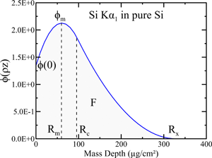
To determine the composition of bulk samples, the emitted primary characteristic X-ray intensity can be evaluated using the so-called ϕ(ρz) distribution, describing the ionization depth distribution of a given electron shell of a given element by electron impact in a material. Several ϕ(ρz) models have been developed over the years. For a comprehensive review of the existing models used for bulk analysis, see Lavrent'ev et al. (Reference Lavrent'ev, Korolyuk and Usova2004). In the present work, the primary X-ray intensity emitted from a sample is calculated using the PAP ionization depth distribution as described in Pouchou & Pichoir (Reference Pouchou, Pichoir, Heinrich and Newbury1991). The main properties of the model are presented here. The PAP model is composed of two connected parabolas (see Fig. 2) representing the ionization depth distribution along the target mass depth:
 $$\phi \lpar {\rho {z}} \rpar = \left\{{\matrix{ {A_1{\lpar {\rho z-R_{\rm m}} \rpar }^2 + B_1} \hfill & {\hbox{\,for}\;0 \lt \rho z \le R_{\rm c}} \hfill \cr {A_2{\lpar {\rho z-R_{\rm x}} \rpar }^2} \hfill & {\hbox{\,for}\;R_{\rm c} \lt \rho z \lt R_{\rm x}} \hfill \cr } } \right.$$
where ρz is the mass depth as previously defined. R m is the mass depth at which the ϕ(ρz) distribution reaches its maximum, R c is the mass depth at which the two parabolas are connected, and R x is the maximum mass depth at which the ionization ceases.

Fig. 2. Example of ϕ(ρz) distribution versus the mass depth calculated by the PAP model for the Si Kα 1 X-ray line generated in pure Si at 10 kV. The parameters of the ϕ(ρz) distribution, R m, R x, ϕ(0) (the surface ionization), and F (integrated area under the curve), are also indicated.
The PAP model was developed to agree with the definition of the ϕ(ρz) distribution given by Castaing (Reference Castaing1951): the area F of the ϕ(ρz) distribution is proportional to the total number N j of primary ionizations produced per incident electron in the electron shell j of the studied atom. Following this definition, N j can be expressed by:
 $$N_j = \displaystyle{{C_i} \over {A_i}}\;N_{\rm A}\;{ \sigma }_j\lpar {E_0} \rpar \;F,$$
where C i, N A, A i, and σj(E 0) are quantities previously defined, and F is the area of the ϕ(ρz) distribution:
 $$F = \int_0^\infty {\phi \lpar {\rho z} \rpar d\rho z} .$$
The parameter F can be calculated by expressing the total number of primary ionizations N j by means of a backscatter loss factor R and a deceleration (stopping) factor 1/S:
 $$N_j = C_i\;\displaystyle{{N_{\rm A}} \over {A_i}}R\displaystyle{1 \over S}$$
with
 $$\displaystyle{1 \over S} = \int_{E_0}^{E_c} {\sigma _j\lpar E \rpar /\lpar {dE/d{ \rho s}} \rpar \;dE} $$
where dE/dρs represents the electron stopping power (i.e., loss of energy of the electrons along their trajectories) and E c is the ionization energy of the electron shell of interest. The ionization cross-section σ j(E) model used by Pouchou and Pichoir in developing their model is that of Hutchins (Reference Hutchins, Kane and Larrabee1974):
 $${ \sigma }_j\lpar E \rpar = cst\;\displaystyle{{\ln \lpar {E/E_c} \rpar } \over {{\lpar {E/E_c} \rpar }^m\;E_c^2 }}$$
with cst being a constant and m = 0.86 + 0.12 exp( − (Z/5)2) for the K shell, m = 0.82 for the L shell, and m = 0.78 for the M shell. The term Z represents the atomic number of the considered element.
The term 1/S can easily be calculated using the continuous slowing down approximation. To model the deceleration factor, Pouchou and Pichoir have used a modified version of Bethe's law for low energy electrons:
 $$\displaystyle{{dE} \over {d{\rho s}}} = -\displaystyle{M \over J}\;\displaystyle{1 \over {\,f\lpar V \rpar }},$$
where  $M = \sum\nolimits_i {C_iZ_i/A_i}$ and $J = \hbox{exp}\left({\sum\nolimits_i {\lpar C_iZ_i/A_i\rpar } \ln \lpar {J_i} \rpar /M} \right)$ with the index i running through the number of elements composing the studied material. J i is the mean ionization potential, in keV, as obtained by Zeller and cited by Ruste & Gantois (Reference Ruste and Gantois1975):
 $$J_i = 10^{-3}Z_i\lpar {10.04 + 8.25\, {\rm e}^{-Z_i/11.22}} \rpar .$$
The term f(V) is described by:
 $$f\lpar V \rpar = \sum\limits_{k = 1}^3 {D_kV^{P_k}}, $$
where V = E/J, D 1 = 6.6 × 10⁻⁶, D 2 = 1.12 × 10⁻⁵(1.35 − 0.45J 2), D 3 = 2.2 × 10⁻⁶/J, P 1 = 0.78, P 2 = 0.1, and P 3 = 0.25J − 0.5.
Thus, the term 1/S can easily be obtained by calculating the above integral [equation (7)]:
 $$\eqalign {\displaystyle{1 \over S}} =& \displaystyle{J \over {E_cM}}\sum\limits_{k = 1}^3 D_k{{\left({\displaystyle{{E_c} \over J}} \right)}^{P_k}}\cr &{\displaystyle{{{\lpar {E_0/E_c} \rpar }^{1 + P_k-m} \times \lpar {\lpar {1 + P_k-m} \rpar \ln \lpar {E_0/E_c} \rpar -1} \rpar + 1} \over {{\lpar {1 + P_k-m} \rpar }^2}}. $$
In equation (6), the backscatter loss factor R is defined by:
 $$R = 1-\bar{\eta }\;\bar{W}\;\lpar {1-G\lpar {U_0} \rpar } \rpar, $$
where  $\bar{\eta }$ is the mean backscatter coefficient defined as:
 $$\bar{\eta } = 1.75 \times 10^{-3}\overline {Z_b} + 0.37\lpar {1-{\rm e}^{-0.015\;{\overline {Z_b} }^{1.3}}} \rpar $$
with the mean atomic number calculated as  $\overline {Z_b} = \left({\sum\nolimits_i {C_iZ_i^{0.5} } } \right)^2$.
The term  $\bar{W}$ is the mean reduced energy of the backscattered electrons and is defined as:
 $$\bar{W} = 0.595 + \displaystyle{{\bar{\eta }} \over {3.7}} + \bar{\eta }^{4.55}.$$
The term G(U 0) is given by:
 $$G\lpar {U_0} \rpar = \displaystyle {\left({U_0-1-\displaystyle{{1-1/U_0^{1 + q} } \over {1 + q}}} \right) \over {\lpar {2 + q} \rpar \;h\lpar {U_0} \rpar } }, $$
where U 0 is the overvoltage U 0 = E 0/E c, h(U 0) = 1 + U 0 (ln(U 0) − 1), and  $q = \lpar {2\bar{W}-1} \rpar /\lpar {1-\bar{W}} \rpar$.
Having obtained the factor R and 1/S, the area F can be calculated from equations (4) and (6) by:
 $$F = R\;\displaystyle{1 \over S}\,\displaystyle{1 \over {{ \sigma }_j\lpar {E_0} \rpar }},$$
where σj(E 0) is the electron impact ionization cross section previously defined. Using the ionization cross-section model of Hutchins, Pouchou and Pichoir adjusted the PAP algorithm such that it reproduced a number of experimental measurements. Hence, to calculate the parameters 1/S and F, this model of ionization cross section must be used when calculating the ϕ(ρz) distribution and should not be replaced with a different one (e.g., a more recent, more accurate model). However, once the ϕ(ρz) distribution is calculated, to obtain the absolute X-ray intensities [see equation (1)], it is possible to use a different model of electron impact ionization cross sections. Indeed, the main goal of the PAP model is to describe the ϕ(ρz) distribution. The atomic parameters used to convert the number of ionizations to the number of emitted X-rays [the left terms outside of the integral in equation (1)], that is, the fluorescence yield, the transition probability, and the ionization cross section, are not directly linked to the PAP model and can be replaced by different models. Furthermore, in most cases, when calculating the k-ratio, they will cancel out. Also, notice that this expression of F [equation (17)] is slightly different from equation (13) in Pouchou & Pichoir (Reference Pouchou, Pichoir, Heinrich and Newbury1991), which was presumably incorrectly reported, but is in accordance with equations (2) and (3) from the same publication.
In equation (3), the terms A 1, A 2, and B 1 are parameters that can generally be determined by solving the set of equations describing the ϕ(ρz) distribution and by noting the surface ionization ϕ(0), that is, the value of the ϕ(ρz) distribution at the surface of the sample:
 $$A_1 = \displaystyle{{\phi \lpar 0 \rpar } \over {{R_{\rm m}\left({R_{\rm c}-R_{\rm x}\left({\displaystyle{{R_{\rm c}} \over {R_{\rm m}}}-1} \right)} \right)}}},$$
 $$B_1 = \phi \lpar 0 \rpar -A_1R_{\rm m}^2, $$
 $$A_2 = A_1\displaystyle{{R_{\rm c}-R_{\rm m}} \over {R_{\rm c}-R_{\rm x}}}.$$
The expressions for R c, R x, R m, and ϕ(0) are as follow:
 $$R_{\rm c} = 1.5\;\left[{\displaystyle{{F-\lpar {\phi \lpar 0 \rpar R_{\rm x}/3} \rpar } \over {\phi \lpar 0 \rpar }}-\displaystyle{{\sqrt d } \over {\phi \lpar 0 \rpar \lpar {R_{\rm x}-R_{\rm m}} \rpar }}} \right]$$
with
 $$d = \lpar {R_{\rm x}-R_{\rm m}} \rpar \left({F-\displaystyle{{\phi \lpar 0 \rpar R_{\rm x}} \over 3}} \right)\left[{\lpar {R_{\rm x}-R_{\rm m}} \rpar F-\phi \lpar 0 \rpar R_{\rm x}\left({R_{\rm m} + \displaystyle{{R_{\rm x}} \over 3}} \right)} \right],$$
 $$\phi \lpar 0 \rpar = 1 + 3.3\left({1-\displaystyle{1 \over {U_0^{2-2.3\bar{\eta }} }}} \right)\bar{\eta }^{1.2}.$$
The term R x represents the range of ionization and is given by:
 $$R_x = Q\,D\,R_0$$
with
 $$Q = Q_0 + \lpar {1-Q_0} \rpar \;{\rm e}^{-\lpar \lpar U_0-1\rpar /b\rpar },$$
where  $b = 40/\bar{Z}$ and $\bar{Z} = \sum\nolimits_i {C_iZ_i} .$
The factor Q 0 is given by:
 $$Q_0 = 1-0.535{\rm e}^{-{\lpar {21/\overline {Z_n} } \rpar }^{1.2}}-2.5 \times 10^{-4}\left({\displaystyle{{\overline {Z_n} } \over {20}}} \right)^{3.5}$$
with  $\ln \overline {Z_n} = \sum\nolimits_i {C_i\ln \lpar {Z_i} \rpar }$ or in a more concise form: $\overline {Z_n} = \mathop \prod \nolimits_i Z_i^{C_i}$.
The factor D is expressed by:
 $$D = 1 + \displaystyle{1 \over {U_0^{{\bar{Z}}^{0.45}} }}.$$
The term R 0 represents the maximum mass–distance traveled by an electron until its energy reaches the ionization energy Ec of the considered electron shell. R 0 can be obtained by integrating the slowing down equation [equation (9)] from E 0 to E c:
 $$\int_{E_0}^{E_c} {\,f\left({\displaystyle{E \over J}} \right)\displaystyle{J \over M}\;dE} = - \int_0^{R_0} {d\rho s}. $$
Hence, using equation (11) to describe f(E/J):
 $$R_0 = \displaystyle{1 \over M}\sum\limits_{k = 1}^3 {J^{1-P_k}D_k\displaystyle{{E_0^{P_k + 1} -E_c^{P_k + 1} } \over {P_k + 1}}}. $$
Finally, R m is given by:
 $$R_{\rm m} = G_1\lpar {\bar{Z}} \rpar \times G_2\lpar {U_0} \rpar \times G_3\lpar {U_0\comma \;\bar{Z}} \rpar \times R_{\rm x}$$
with
 $$G_1\lpar {\bar{Z}} \rpar = 0.11 + 0.41\hbox{e}^{-{\lpar {\bar{Z}/12.75} \rpar }^{0.75}},$$
 $$G_2\lpar {U_0} \rpar = 1-\hbox{e}^{-\lpar {\lpar U_0-1\rpar }^{0.35}/1.19\rpar },$$
 $$G_3\lpar {U_0\comma \;\bar{Z}} \rpar = 1-\hbox{e}^{-\lpar \lpar \lpar U_0-0.5\rpar {\bar{Z}}^{0.4}\rpar /4\rpar }.$$
The terms R c, R x, R m, and ϕ(0) can then be used to calculate the ϕ(ρz) ionization distribution of a given electron shell (or subshell) of a given element as a function of the mass depth. In some cases, at very small overvoltages, that is, U 0 very close to one, it is possible that equation (21) has no real solution because the discriminant d [equation (22)] is negative. In such a case, a value of zero is imposed on d and the equation linking R m to R x [equation (30)] is replaced by:
 $$R_{\rm m} = R_{\rm x}\displaystyle{{F-\phi \lpar 0 \rpar R_{\rm x}/3} \over {F + \phi \lpar 0 \rpar R_{\rm x}}}.$$
Hence, equation (21) is replaced by:
 $$R_{\rm c} = 1.5\;R_{\rm m}\displaystyle{{F + \phi \lpar 0 \rpar R_{\rm x}} \over {\phi \lpar 0 \rpar R_{\rm x}}}.$$
At very low overvoltages, the ϕ(ρz) distribution may also have its maximum at the surface of the sample (at mass depth ρz = 0). This leads to unrealistic values of R m, that is, R m < 0 or R m > R x. In such a case, the ϕ(ρz) distribution can be described by a decreasing exponential or by a sum of an exponential and a parabola. For more details, see Pouchou & Pichoir (Reference Pouchou, Pichoir, Heinrich and Newbury1991).
Fluorescence
The term fluorescence refers to the production of characteristic X-rays by other characteristic X-rays, the characteristic fluorescence, or by bremsstrahlung X-rays, the bremsstrahlung fluorescence, coming from the same phase. Similarly, the term secondary fluorescence is defined by the production of characteristic X-rays by other characteristic X-rays, the characteristic secondary fluorescence, or by X-rays from the continuum, the bremsstrahlung secondary fluorescence, from another phase (in the case of nonhomogeneous samples such as thin films or embedded particles). In some cases, the fluorescence cannot be neglected and can account up to ~10% of the total X-ray intensity. The methods used to calculate the fluorescence are detailed below.
Characteristic Fluorescence
In the case of bulk samples, the calculation of the fluorescence by characteristic X-rays is straightforward: consider a given element i and a given characteristic X-ray emitted by i and having an energy greater than the critical ionization energy of the electron shell involved in the production of the considered fluoresced characteristic X-rays. This X-ray depth distribution is given by an equation similar to equation (1):
 $$n_{{\rm el}}\displaystyle{{N_{\rm A}} \over {A_i}}\;C_i\;\sigma _{e_m^- }^i \lpar {E_0} \rpar \lambda _m^i \;\omega _m^i \;\displaystyle{{{\rm \Gamma }_{m-n}^i } \over {{\rm \Gamma }_{m-{\rm total}}^i }}\displaystyle{1 \over {4\pi }}\int_0^\infty {\phi _m^i \lpar {\rho z_0} \rpar d\rho z_0} ,$$
where  $\phi _m^i \lpar {\rho z_0} \rpar$ is the ionization depth distribution of electron shell m of element i present at mass depth ρz 0. The probability of producing an electron vacancy in the shell m by electron impact ionization is given by $\lpar \rho N_{\rm A}/A_i\rpar \;C_i\;\sigma _{e_m^- }^i \lpar {E_0} \rpar \;\lambda _m^i$, where N A is Avogadro's number, A i is the atomic weight of element i, and C i is the concentration (weight fraction) of element i. $\sigma _{e_m^- }^i \lpar {E_0} \rpar$ is the ionization cross section of the shell m of element i by electron impact of energy E 0. The term $\lambda _m^i {\rm \;}$ represents the radiative, nonradiative, Coster–Kronig and super-Coster–Kronig contributions to the production of an electron vacancy in the shell m of element i. Note that the term ρ, the mass thickness of the material, was incorporated in the term dρz 0 in equation (36). A given characteristic X-ray of energy E m−n is emitted during the relaxation of the ionized atom i by transition of an electron from the shell or subshell n to the shell or subshell m. These are represented by the fluorescence yield $\omega _m^i$, the radiative transition probability for an electron to make a transition from shell n to shell m, ${\rm \Gamma }_{m-n}^B$, and the total radiative probability for all possible transitions to the shell m, ${\rm \Gamma }_{m-{\rm total}}^B$. Note that the term 1/4π, which assume an isotropic emission of X-rays, is required to obtain an X-ray distribution in photons per unit of solid angle. The characteristic X-rays of energy E m−n, emitted with a direction θ, as shown in Figure 3, undergo absorption along their path s = (z 0 − z)/cosθ.

Fig. 3. Characteristic fluorescence in a bulk sample. The fluorescing element i emits a characteristic X-ray of energy E m−n at mass depth ρz 0 which will fluoresce element l at mass depth ρz, producing the considered characteristic X-ray of energy E p−q.
Then, the probability for the X-rays to travel a distance s without being absorbed is given by the exponential term  $e^{-\lpar {\mu /\rho } \rpar \lpar {E_{m-n}} \rpar \rho \lpar \lpar z_0-z\rpar /\cos \theta \rpar }$. The absorption of the photons of energy E m−n is represented by the MAC (μ/ρ)(E m−n). The product of the ionization depth distribution by the absorption exponential is integrated over the entire mass depth of the sample, from 0 to ∞.
Then, the probability for the X-rays to be absorbed by atoms of the studied element l (the fluoresced element) in the infinitely small distance ds and to ionize the electron shell (or subshell) p through photoelectric interaction, represented by the photoelectric cross section  $\sigma _{{\rm ph}_p}^l \lpar {E_{m-n}} \rpar$ and radiative, nonradiative, Coster–Kronig and super-Coster–Kronig contributions represented by the term $\lambda _p^l \;$ is given by:
 $$1-{\rm e}^{-\rho \lpar {N_{\rm A}/A_l} \rpar C_l\lambda _p^l \sigma _{{\rm ph}_p}^l \lpar {E_{m-n}} \rpar ds}\approx \displaystyle{{\rho N_{\rm A}} \over {A_l}}C_l\lambda _p^l \sigma _{{\rm ph}_p}^l \lpar {E_{m-n}} \rpar ds.$$
 The term ds can be expressed by ds = dz/cosθ and the term ρ can be incorporated in the term dρz to convert the integration on the depth into integration on the mass depth. The emission of the considered characteristic X-rays produced by element l during the relaxation process from which an electron from the shell q falls into the shell p is taken into account by the fluorescence yield  $\omega _p^l$ and radiative transition probability ${\rm \Gamma }_{p-q}^l /{\rm \Gamma }_{p-{\rm total}}^l$. A term 1/4π is also required to obtain an X-ray distribution in photons per unit of solid angle. The attenuation of these X-rays of energy E p−q emitted toward the detector with an angle θ d is taken into account by an exponential term with an MAC $\lpar {\mu /\rho } \rpar \lpar {E_{p-q}} \rpar \colon\; \hbox{e}^{-\lpar {\mu /\rho } \rpar \lpar {E_{p-q}} \rpar \rho z/\sin \theta _d}$.
Finally, the probability of detection of the emitted X-rays by the spectrometer is represented by the terms ɛ and Ω, where ɛ is the intrinsic detection efficiency and Ω is the solid angle subtended by the detector.
By assuming the X-ray emission being isotropic, the emission of X-rays of energy E m−n is integrated using spherical coordinates and using the infinitesimal element of solid angle dΩ = sinθdθdφ. Two cases must be distinguished: the fluorescing X-rays of energy E m−n are emitted in the upward direction (toward the surface of the sample) or in the downward direction. In the first case, the variable θ is integrated from π/2 to π and the variable φ is integrated from 0 to 2π. The mass depth ρz is, therefore, integrated from 0 to ρz 0. In the second case, the variable θ is integrated from 0 to π/2 , the variable φ is integrated from 0 to 2π and the mass depth ρz is integrated from ρz 0 to ∞. Because all the described terms are independent of the variable φ and because of the symmetry of the  $\phi _m^i \lpar {\rho z_0} \rpar$ distribution around the ρz 0 axis, the integral over the angle φ is equal to 2π. In both cases, the integration is performed over a solid angle of 2π steradians.
Lastly, the total fluorescence produced by characteristic X-rays is given by summing the contributions from all the characteristic X-rays, produced by the element of interest as well as all other elements present in the material, with an energy greater than the critical ionization energy of the electron shell involved in the production of the considered characteristic X-rays. The total characteristic fluorescence, from X-rays of energy E m−n emitted in the upward direction, is then given by:
 $$\eqalign{{\cal F}_{\rm c}& = \sum\limits_{i = 1}^N {\sum\limits_{m\comma n} {n_{{\rm el}}\displaystyle{{N_{\rm A}} \over {A_i}}\;C_i\;\sigma _{{e}_m^- }^i \lpar {E_0} \rpar \lambda _m^i \;\omega _m^i \;\displaystyle{{{\rm \Gamma }_{m-n}^i } \over {{\rm \Gamma }_{m-{\rm total}}^i }} \times \displaystyle{1 \over {4\pi }}} } \cr & \quad \times \displaystyle{{N_{\rm A}} \over {A_l}}C_l{\rm \;}\sigma _{{\rm ph}_p}^l \lpar {E_{m-n}} \rpar \lambda _p^l \;\omega _p^l \displaystyle{{{\rm \Gamma }_{p-q}^l } \over {{\rm \Gamma }_{p-{\rm total}}^l }}\displaystyle{1 \over {4\pi }}{\rm \;}2{\rm \pi \;} \cr & \quad \times \;\int_{\theta = \pi /2}^\pi {\int_{\rho z_0 = 0}^\infty {\int_{\rho z = \rho z_0}^0 {\phi _m^i \lpar {\rho z_0} \rpar \hbox{e}^{-\lpar {\mu /\rho } \rpar \lpar {E_{m-n}} \rpar \rho \lpar \lpar z_0-z\rpar /\cos \theta \rpar }}}}\cr & \quad\times\hbox{e}^{-\lpar {\mu /\rho } \rpar \lpar {E_{p-q}} \rpar \lpar {\rho z/\sin \theta_d} \rpar }\sin \theta \displaystyle{{d\rho z} \over {\cos \theta }}d\theta \;d\rho z_0\;\varepsilon \;{\rm \Omega } ,} $$
where the index i goes through all the N elements in the material. The indexes m and n represent the final and initial electron shells (subshells) of the electron transition producing the characteristic X-ray of the element i that will fluoresce the considered element l, respectively. Note that the characteristic X-ray emitted by an electron transition from the shell n to the shell m must have an energy E m−n greater than the critical ionization energy of the electron shell involved in the production of the considered characteristic X-rays. A similar equation is obtained in the case where the X-rays of energy E m−n from the fluorescing element are emitted in the downward direction.
The analytical resolution of this equation is possible when using the PAP ionization distribution model. For more details on the resolution of this equation, see Waldo (Reference Waldo and Howitt1991) and Supplementary Material.
Bremsstrahlung Fluorescence
Our implementation of the fluorescence created by the bremsstrahlung is here different from the usual simplistic assumption that the bremsstrahlung X-rays are produced at a point on the surface of the sample or surface of the considered layer (Pouchou & Pichoir, Reference Pouchou, Pichoir, Heinrich and Newbury1991). Instead, a ϕ(ρz) distribution is calculated for an “imaginary” element having a characteristic X-ray with a critical ionization energy E c equal to the energy of the bremsstrahlung photon considered. This phi-rho-z distribution, φ Brem(ρz;E ph), represents the intensity of production of bremsstrahlung photons of energy E ph as a function of the mass depth ρz for a given material and electron beam energy. These bremsstrahlung phi-rho-z curves are then integrated over the depth of the specimen to calculate fluorescence, following the same scheme as for the characteristic fluorescence. The process is iterated over a discretized subset of bremsstrahlung energies, from the ionization threshold up to the energy of the primary electrons, E 0. Because the X-ray spectrum can be strongly modified by the absorption edges of the elements constituting the specimen, the considered total energy range (from 0 to E 0) is divided into energy subsets in which no absorption edge is present (i.e., the limits of the energy subsets are defined by the ionization edges of the elements present in the specimen). In each subset, the total emitted bremsstrahlung fluorescence is calculated by numerical integration performed over five equally spaced energy limits using Simpson's integration rule.
However, the bremsstrahlung ϕ(ρz) distributions calculated with the PAP model are a rough approximation of the real bremsstrahlung φ Brem(ρz;E ph) distribution. To help correcting the differences, the shape of the emitted X-ray spectrum as a function of the X-ray energy, only taking into account X-rays produced by bremsstrahlung fluorescence, is multiplied by the shape of the bremsstrahlung spectrum (spectral distribution I(E)) given by Small et al. (Reference Small, Leigh, Newbury and Myklebust1987) and modified by Kulenkampff [as cited in Pouchou & Pichoir (Reference Pouchou, Pichoir, Heinrich and Newbury1991)]:
 $$I\lpar E \rpar = q\,e^B\left[{\bar{Z}\left({\displaystyle{{E_0} \over E}-1} \right)} \right]^M + C\bar{Z}^2,$$
where q = 10−8 keV−1 as proposed by Pouchou & Pichoir (Reference Pouchou, Pichoir, Heinrich and Newbury1991), B = −3.22 × 10⁻² × E 0 + 5.8, M = 5.99 × 10⁻³ × E 0 + 1.05, and C = 6 × 10⁻¹⁰.  $\bar{Z}$ is the mean atomic number of the material calculated by $\bar{Z} = \sum\nolimits_{i = 1}^N {C_iZ_i}$, where N represents the number of elements in the material and C i and Z i are quantities previously defined. This method, despite being more refined than the point surface method [where all the bremsstrahlung is generated at the surface of the layer as described in Pouchou & Pichoir (Reference Pouchou, Pichoir, Heinrich and Newbury1991)], seems to overestimate the produced values when compared to Monte Carlo simulations.
To further improve the calculated bremsstrahlung fluorescence values, two empirical parameters were introduced in the calculation algorithms: the first parameter, denoted as α, artificially modifies the energy of the primary electrons in equation (39) describing I(E) and also in the calculation of the bremsstrahlung ϕ(ρz) distributions with the PAP model. The second parameter, denoted as β, modifies the value of the constant q previously defined in equation (39). The values of these two parameters were obtained by adjusting the calculated fluorescence values to bremsstrahlung fluorescence data obtained by Monte Carlo simulations using the code PENEPMA (Llovet & Salvat, Reference Llovet and Salvat2017) for pure elements using the Kα, Lα, and Mα X-ray lines. For each X-ray line, the determined parameter values were fitted by parts against the element's atomic number Z with a polynomial function, as shown in Figure 4. Good coefficients of determination R 2 were obtained for all the fitting polynomial functions except for the coefficient β for the Mα X-ray lines where it degrades to R 2 = 0.858 due to the large scattering of the data points. The extracted polynomials were then implemented in our algorithm to predict the fluorescence produced by the bremsstrahlung. It is worth noting that the discontinuities for the Lα lines seem to correspond to the population of the electron shells of the different elements. However, this behavior is not reproduced for the Kα and Mα lines.

Fig. 4. Values of the α and β coefficients used to improve the bremsstrahlung fluorescence for the Kα, Lα, and Mα X-ray lines. The symbols are the values obtained by fitting the coefficients to the results obtained by Monte Carlo simulations. The continuous lines represent the fit of the determined coefficients over the atomic number Z.
BadgerFilm: Good for Bulk as Well as for Thin Films
The described algorithms were implemented in a graphical user interface program called BadgerFilm, whose main goal is thin film analysis but is robust enough to work well for “normal bulk” EPMA. Given the lack of thin film reference materials for a critical evaluation of its thin film accuracy, whereas there is a very large set of data for evaluating bulk materials, these bulk data will be used for the evaluation below. First, we describe here some relevant features of BadgerFilm.
The program allows the user to easily select the different parameters required to calculate film thicknesses and compositions, as well as the composition of the substrate, such as the takeoff angle, the MAC dataset, or the ionization cross sections (Fig. 5). The experimental data (element, X-ray line, experimental k-ratio, uncertainty on the k-ratio, and accelerating voltage) can easily be entered by the user in the software by copy-paste actions. k-ratios can be defined relative to a compound standard as well as a pure elemental standard that has been previously defined using BadgerFilm. Layer thicknesses and compositions can also be fixed if known. BadgerFilm uses a nonlinear fitting algorithm based on the Levenberg–Marquardt fitting algorithm (Levenberg, Reference Levenberg1944; Marquardt, Reference Marquardt1963) to calculate k-ratios and to iterate on the compositions and thicknesses of the films (and substrate) until the theoretical k-ratios match the experimental k-ratios. In more detail, the fitting algorithm tries to minimize a set of equations—here, it minimizes the difference between experimental k-ratios and analytical calculated k-ratios—by adjusting a set of parameters. In our case, the parameters are the concentrations of the different elements and the thickness of the different layers (in the general case of a multilayer specimen). By considering a multilayered specimen composed of i different elements (counted several times if present in several layers or substrate) and j different layers, and a number m of experimental k-ratios (recorded for different elements, X-ray lines, and accelerating voltages), the set of m equations to minimize is:
 $$k_m^{\rm th} \lpar {C_1\comma \;C_2\comma \;\ldots \comma \;C_i\comma \;\;d_1\comma \;d_2\comma \;\ldots \comma \;d_j\semicolon \;E_m} \rpar -k_m^{\exp} = 0,$$
where the C i parameters represent the elemental concentrations, the d j parameters represent the layer thicknesses, and E m represents the electron beam energy at which the m k-ratio was measured.  $k_m^{\rm th}$ is the theoretical k-ratio calculated with the chosen ϕ(ρz) model and $k_m^{{\exp}}$ represents the corresponding experimental k-ratio. To help the algorithm converge to the “best” solution, BadgerFilm implements, as an option, another set of equations which is added to the existing equations. These extra equations state that the sum of the different elemental concentrations in each layer (or the substrate) should be as close as possible to 100 wt%. For example, for the layer j, this can be expressed as:
 $$\mathop \sum \limits_{\matrix{ {l = 1} \cr {elt\;l \, \in \,{\rm layer}\,j} \cr } }^i C_l-1 = 0,$$
where the sum goes through all the elemental concentrations for the elements present in the layer j. However, this set of equations will not force the total concentration to be equal to 100 wt% (by opposition to a normalization procedure that will force the results to be 100 wt%) but will help the fitting algorithm to go toward the “best” solution. A missing element or an incorrect k-ratio in the analysis can still lead to a total concentration lower or more than 100 wt%. This option can be deactivated by the user at any time.

Fig. 5. The BadgerFilm graphical user interface allows to easily analyze EPMA experimental data, here for a bulk Al0.398Ti0.602 alloy.
The calculation's results are displayed in a scrollable text box and are given with an uncertainty on the results. These uncertainties are calculated by the user, previously, from the experimental k-ratios uncertainties (by default these uncertainties are set to 5%, corresponding to uncertainties on the recorded X-ray intensities of 3.5% for both the unknown and the standard, with the user free to set more appropriate values) which are propagated by the fitting algorithm to give uncertainties on the fitted parameters. These uncertainties do not take into account the uncertainties associated with the atomic parameters and with the ϕ(ρz) model (Ritchie & Newbury, Reference Ritchie and Newbury2012; Ritchie, Reference Ritchie2020). The experimental k-ratios and the fitting results are also plotted in a graph to offer a quick visualization of the correctness of the fit. The data can be saved into a BadgerFilm text file format and easily reloaded later. The program also allows the user to import files in the STRATAGem (STRATAGem version 6.2) format, enabling compatibility with STRATAGem and Probe for EPMA (Donovan et al., Reference Donovan, Kremser, Fournelle and Goemann2020). The calculated data can easily be exported to a spreadsheet program in a convenient preformatted way.
The implemented algorithm to calculate the characteristic fluorescence considers a total of 24 characteristic X-ray lines as possible sources of fluorescence (under the condition that the energy of the X-ray line is greater than the ionization threshold of the studied X-ray transition), namely Kα 1, Kα 2, Kβ, Lα 1, Lα 2, Lβ 1, Lγ 1, Lη, Lℓ, L3N5, Mα 1, Mα 2, Mβ 1, Mγ 1, M4O6, M3O5, M2N4, M2N1, M3O1, M3O4, M1N2, M1N3, M2O4, and M1O2.
The relaxation parameters, MACs and ionization cross sections used by default in BadgerFilm to predict the emitted X-ray intensity, are the same as the atomic parameters used in the general-purpose Monte Carlo code PENELOPE 2018 (Salvat, Reference Salvat2019), and therefore, in PENEPMA (Llovet & Salvat, Reference Llovet and Salvat2017), a program that uses the subroutines of PENELOPE to simulate X-ray spectra and quantities of interest for microanalysis by EPMA. This allows the user to directly compare the predictions of BadgerFilm with the predictions of PENEPMA. The default MACs used in BadgerFilm are the PENELOPE 2018 MACs, which were calculated from the photoelectric cross section of Sabbatucci & Salvat (Reference Sabbatucci and Salvat2016). The probability to produce the studied characteristic X-rays per incident electron (of energy E 0) is given by the electron impact X-ray production cross section σ X(E 0) = ω j (Γj−k/Γj−total) λ j σ j(E 0) (Moy et al., Reference Moy, Merlet, Llovet and Dugne2013), where the atomic parameters ω j, Γj−k, Γj−total, and λ j are extracted from the LLNL Evaluated Atomic Data Library (EADL) tables (Perkins et al., Reference Perkins, Cullen, Chen, Rathkopf, Scofield and Hubbell1991). As previously defined, the term λ j takes into account the production of electron vacancies in the studied electron shell (or subshell) by ionization of other more inner shells (or subshells) and subsequent relaxations by Auger, Coster–Kronig, super-Coster–Kronig, and radiative intra-shell transitions that lead, by one or multiple steps, to a vacancy in the electron shell of interest. The probabilities associated with these relaxation transitions are also extracted from the EADL tables. The electron impact ionization cross sections σ j(E 0) are calculated from the model of Bote & Salvat (Reference Bote and Salvat2008). It is important to note that the electron impact ionization cross sections used in the calculation of the ϕ(ρz) ionization depth distribution with the PAP algorithm (necessary to calculate the area F of the ϕ(ρz) distribution) are based on the Hutchins model (Hutchins, Reference Hutchins, Kane and Larrabee1974) and were not replaced by any other model, as they are intrinsically related with the good performance of the PAP algorithm. The X-ray line energies are calculated from the difference of energy between the ionization energy of the electron shells (or subshells) giving rise to the studied characteristic X-rays. The ionization energies employed in BadgerFilm are those used in PENELOPE 2018 and originally extracted from Carlson (Reference Carlson1975).
BadgerFilm offers the possibility to select other atomic parameter models: the MAC30 model derived by Heinrich (Reference Heinrich, Brown and Packwood1987) or the MACs calculated from the photoelectric cross sections extracted from the LLNL Evaluated Photon Data Library (EPDL97) (Cullen et al., Reference Cullen, Hubbell and Kissel1997). Experimental MAC values can also be specified for a particular emitter element and X-ray line and for a particular absorber element. In addition, the ionization cross-section model of Hutchins (Reference Hutchins, Kane and Larrabee1974) can be selected to calculate the term σ j(E 0) in equation (1).
Test of the Implemented Models for Bulk Materials
The predictions of the implemented algorithms described above were tested on the 826 k-ratio entries compiled and tabulated by Pouchou & Pichoir (Reference Pouchou, Pichoir, Heinrich and Newbury1991). This database contains k-ratios measured on binary bulk standards of known compositions, at different accelerating voltages ranging from 2.5 to 48.5 kV and for different detector takeoff angles varying from 40° to 75°. Comparisons were made using different MACs, different ionization cross-section models (only to calculate the absolute X-ray intensity, not to calculate the ϕ(ρz) distribution) and with or without fluorescence (Fig. 6). Theoretical k-ratios were compared to the tabulated measured k-ratios and their ratios plotted with histograms with a bin size of 0.5%.

Fig. 6. Comparison of the results with our modified PAP algorithm with the original published data from Pouchou & Pichoir (Reference Pouchou, Pichoir, Heinrich and Newbury1991). (a) Uses the MACs from the MAC30 database (Heinrich, Reference Heinrich, Brown and Packwood1987) with no fluorescence considered. (b–d) Use the MACs extracted from PENELOPE 2018. (b) Only considers the fluorescence by characteristic X-rays, (c) only the fluorescence by the bremsstrahlung, and (d) both fluorescence by the characteristic X-rays and by the bremsstrahlung.
The implemented ϕ(ρz) algorithm used in BadgerFilm was compared to the original bulk data of Pouchou and Pichoir using the MACs of Heinrich, MAC30 (Heinrich, Reference Heinrich, Brown and Packwood1987) which they used and no fluorescence (they used none). The BadgerFilm results are very similar to the original data. However, some discrepancies exist: our distribution, centered on 1.0, is sharper (less broadened) in the central part but has larger tails; also note that the histogram plotted by Pouchou and Pichoir clearly has more than the 826 entries tabulated in their 1991 publication (rather, approximately 878 values in their published histogram). The differences between the two histograms, from Pouchou and Pichoir's calculations and BadgerFilm calculations, can be attributed to slightly different characteristic X-ray energies used to calculate the k-ratios, leading to slightly different X-ray absorptions. In addition, our implementation considers the sum of the Kα 1 and Kα 2 X-ray lines rather than just the weighted average Kα line, and thus two different X-ray energies (in a similar way, we also consider the Lα 1 and Lα 2 lines and the Mα 1 and Mα 2 lines for the Lα and Mα lines, respectively). Also different MAC values than the ones produced by the MAC30 algorithm were used for the very light and light elements in the Pouchou and Pichoir's calculations [see Appendix 5 in Pouchou & Pichoir (Reference Pouchou, Pichoir, Heinrich and Newbury1991)]. Rounding errors due to different algorithm implementations, and in a lesser extent due to different programming languages and computer architectures, may also contribute to these differences.
When using the electron impact ionization cross sections of Bote & Salvat (Reference Bote and Salvat2008) and the MACs extracted from PENELOPE 2018, excellent results are obtained when only the fluorescence by characteristic X-rays is considered. The calculation seems to slightly overestimate the k-ratios compared to the original data. Good results are also obtained when only the fluorescence by the bremsstrahlung is considered. In this case, the distribution is slightly broadened compared to the two previous cases. When both contributions to the fluorescence are considered, the results slightly deteriorate with a larger portion of overestimated k-ratios. This deterioration had already been observed by Pouchou & Pichoir (Reference Pouchou and Pichoir1993) when including the fluorescence by the bremsstrahlung into the matrix correction procedure. The reason is that the ϕ(ρz) models, which do not explicitly include the fluorescence effects, have been adjusted during their development on experimental data that contains X-ray intensities produced by fluorescence.Footnote 2 However, despite the broadening of the histogram, the maximum of the distribution is still centered on 1.0, and the mean and standard deviation of the distribution are 1.0050 and 2.58% respectively. Despite giving less satisfactory results, the fluorescence and secondary fluorescence by the characteristic X-rays and by the bremsstrahlung must be considered when analyzing thin films as their contributions to the total produced characteristic X-ray intensity is often not negligible. For example, estimations from Monte Carlo simulations show that at 20 kV, for a film of 100 nm of FeSi2 on top of a Cu substrate, 5 and 1.5% of the Fe Kα X-ray intensity will be produced by the combined effects of fluorescence and secondary fluorescence from the characteristic X-rays and by the bremsstrahlung, respectively.
X-Ray Intensity Predictions: Comparison to Experimental Data
To demonstrate its accuracy, the implemented ϕ(ρz) calculation method must be validated against experimental measurements, when available. BadgerFilm predictions were compared to absolute X-ray intensities emitted from simple pure elements and from binary compounds.
The proposed phi-rho-z implementation was designed to employ the same atomic parameters used in the Monte Carlo code PENEPMA (Llovet & Salvat, Reference Llovet and Salvat2017) allowing a direct comparison of the calculated X-ray intensities in absolute values of photon per electron per steradian with experimental data or Monte Carlo simulations.
Only few experimental absolute X-ray intensities produced by electron beams at normal incidence have been reported in the literature, mainly because of the difficulty of accurately evaluating the spectrometer detection efficiency and the number of incident electrons used to perform the measurements (Dolby, Reference Dolby1960; Dick et al., Reference Dick, Lucas, Motz, Placious and Sparrow1973; Agarwal & Sparrow, Reference Agarwal and Sparrow1981; Procop, Reference Procop2004; Merlet & Llovet, Reference Merlet and Llovet2006; Moy et al., Reference Moy, Merlet and Dugne2015). The experimental data of Dolby (Reference Dolby1960), Dick et al. (Reference Dick, Lucas, Motz, Placious and Sparrow1973), Agarwal & Sparrow (Reference Agarwal and Sparrow1981), and Procop (Reference Procop2004) are displayed in Figure 7 for the Be K, C K, Al K, Si K, Ti K and Kα, Fe L, Cu K and Kα, and Ge Kα radiations. These data were acquired at various takeoff angles. The K radiations are the sum of the Kα and Kβ radiations, whereas the L radiation is the sum of the Lα, Lβ, L2M1, L1M3, L3N1, and L2N1 radiations. As a general trend, the predictions of BadgerFilm underestimate the experimental data, especially for the light elements Be and C. However, the shape of the curves, represented by the scaled X-ray intensities are in excellent agreement with the experimental data. These scaled curves were obtained by multiplying the original curves by constant terms, thus not changing their shape. It is worth noting that large discrepancies exist between experimental data from different authors, especially for the light element C. Note that the X-ray generation value, in photons per electron per steradian, of 3.40 × 10⁻⁵ derived by Procop (Reference Procop2004) for the Al–K X-rays at 5 kV does not match the data in Figure 13 of the same publication. A value of 7.0 × 10⁻⁵ was extracted from this figure and used to plot the Al–K data in our Figure 7e, giving much better agreement between the prediction of BadgerFilm and the experimental data. Figure 8 shows the absolute X-ray intensity predictions of BadgerFilm compared to experimental data of Merlet & Llovet (Reference Merlet and Llovet2006) and Moy et al. (Reference Moy, Merlet and Dugne2015) recorded with a takeoff angle of 40°. Excellent results were obtained for the Al Kα and Ge Kα X-ray intensities compared to Merlet and Llovet experimental data, up to 25 kV. At higher accelerating voltages, the predictions of BadgerFilm underestimate the experimental Al Kα data by 7%, while the predictions for the Ge Kα intensity remain very good. For the Ge Lα intensity, the predictions of BadgerFilm greatly underestimate the experimental data, the relative error being of 36% at 40 kV. This underestimation is similar to the underestimation observed by these authors using the predictions of PENELOPE (2003 version). As a general trend, BadgerFilm predictions overestimate the experimental data of Moy et al. (Reference Moy, Merlet and Dugne2015) measured on heavy elements. For example, for the U Mα and U Mβ X-ray intensities, the predictions of BadgerFilm overestimate the experimental data by about 10%. These differences seen on heavy elements can be partially attributed to uncertainties in the vacancy transition probabilities and to a lesser extent, in the ionization cross sections and MACs adopted for the present calculations. It is important to keep in mind that most of these uncertainties on the atomic parameters will cancel out when calculating k-ratios and that the shape of the curve is what will have the greatest impact on the quantification results. The shapes of the curves are here in very good agreement between the experimental and theoretical data, as shown by the scaled X-ray intensities.

Fig. 7. Comparison of the predictions of BadgerFilm (dotted curves) with experimental absolute X-ray intensities (symbols) measured with various takeoff angles (TOA) and normal electron beam incidence. The BadgerFilm predictions were scaled (dash-dotted lines) by a multiplicative constant to best match the experimental data. (a) Absolute K X-ray intensities of C and Al, and L X-ray intensity of Fe (Dick et al., Reference Dick, Lucas, Motz, Placious and Sparrow1973; Agarwal & Sparrow, Reference Agarwal and Sparrow1981). (b) Absolute K X-ray intensities measured on Be, Ti, and Cu (Dick et al., Reference Dick, Lucas, Motz, Placious and Sparrow1973). (c) Absolute K X-ray intensities measured on C and Al (Dolby, Reference Dolby1960). (d and e) Absolute K and Kα X-ray intensities measured on C, Al, Si, Ti, Cu, and Ge (Procop, Reference Procop2004).

Fig. 8. Comparison of the predictions of BadgerFilm (dotted curves) with experimental absolute X-ray intensities (symbols) measured on standards with a takeoff angle of 40° and normal electron beam incidence. The BadgerFilm predictions were scaled (dash-dotted lines) by a constant to best match the experimental data. (a and b) Absolute Kα and Lα X-ray intensities measured on Al and Ge (Merlet & Llovet, Reference Merlet and Llovet2006). (c–f) Absolute Mα and Mβ X-ray intensities measured on Au, Pt, Pb, Th, and U (Moy et al., Reference Moy, Merlet and Dugne2015).
X-Ray Intensity Predictions: Comparison to Monte Carlo Simulations
It can also be useful to compare the model's predictions to Monte Carlo simulations as it allows the comparison of not only k-ratios but also of absolute X-ray intensities. It also permits the researcher to separate the emitted primary X-ray intensity from the intensity produced by fluorescence from the characteristic X-rays or from the bremsstrahlung, allowing fluorescence calculation algorithms to be validated.
Comparisons were made with Monte Carlo simulations performed with PENEPMA (2018 version). The interaction mechanisms employed in PENEPMA use scattering models that combine numerical tables with analytical cross-section models. The simulation algorithm is valid for energies ranging from few hundred electronvolts to about 1 GeV. Previous work has demonstrated the good accuracy of the PENEPMA Monte Carlo simulations to predict absolute X-ray intensity values (Moy et al., Reference Moy, Merlet and Dugne2015). Predicted X-ray intensity comparisons were made for primary X-ray intensities, for fluorescence due to characteristic X-rays and for fluorescence due to the bremsstrahlung. Elements ranging from C to Am, and electron beam energies ranging from 5 to 30 kV have been used to perform the comparisons. The X-ray lines considered, when available, were the Kα, Lα, and Mα lines. As shown in Figure 9, there is a very good agreement between the Monte Carlo simulations and the BadgerFilm predictions for the Kα X-ray lines for both the primary X-ray intensity and for the fluorescence produced by the bremsstrahlung. Both the shape and the magnitude of the curves are well reproduced by the predictions. For the Lα X-ray intensities, the predictions correctly reproduce the Monte Carlo simulations for the primary X-rays and fluorescence produced by the bremsstrahlung, while the predictions of the fluorescence produced by the characteristic X-rays underestimate the simulations for all the elements. The results for the Mα X-ray lines are more varied: the primary X-ray intensities, as well as the fluorescence produced by the characteristic X-rays, calculated by BadgerFilm are underestimated at high accelerating voltages (>20 kV). The fluorescence generated by the bremsstrahlung is in good agreement with the Monte Carlo simulations except for the element Am where the predictions are overestimated at high kV. It is worth noting that these discrepancies will partially cancel out when calculating the k-ratios. It should also be noted that the BadgerFilm results agree better with the Monte Carlo simulation results than the experimental results. This can be partially due to the fact that, despite using different calculation methods, BadgerFilm and PENEPMA are using the same atomic parameters.

Fig. 9. Primary characteristic X-rays intensities and fluorescence in pure element bulk samples generated by the characteristic X-rays and by the bremsstrahlung, calculated for the Kα, Lα, and Mα X-ray lines by BadgerFilm. The predictions of BadgerFilm (curves) are compared to Monte Carlo simulation results (symbols) obtained using the PENEPMA code. Note that there is no fluorescence by characteristic X-rays for the Kα lines in pure materials.
k-Ratio Predictions: Bulk Compounds
Predictions have also been tested on experimental data for bulk binary samples used in the compilation of Pouchou & Pichoir (Reference Pouchou, Pichoir, Heinrich and Newbury1991). It should be noted that in this section, the thin film programs BadgerFilm and STRATAGem were used in “bulk” mode, that is, with no film, only considering the substrate. As an example, the binary compound Al0.398Ti0.602 (wt fract.) was studied. Ti Kα and Al Kα k-ratios were calculated at different accelerating voltages using several programs: BadgerFilm, STRATAGem, CalcZAF,Footnote 3 (Donovan et al., Reference Donovan, Kremser, Fournelle and Goemann2020), GMRFilm (Waldo, Reference Waldo and Newbury1988), and PENEPMA. Note that the different programs were using the MAC30 MACs (Heinrich, Reference Heinrich, Brown and Packwood1987), except for BadgerFilm and PENEPMA which were using PENELOPE 2018 MAC values. Very good agreement is found between the experimental and calculated Ti Kα k-ratios (Table 1). However, the Al Kα k-ratios, relative to pure Al, seem to be overestimated by the predictions of BadgerFilm (using the PENELOPE 2018 MACs) compared to the originally published experimental data. Note that, when using an MAC value, for the absorption of the Al Kα X-rays by Ti, similar to the value employed in STRATAGem (2,201 cm2/g instead of 2,132 cm2/g), BadgerFilm predicted k-ratios are brought closer to the experimental data, especially at high kV (>30 kV). The same overestimation behavior has been found with the PAP, XPP, and Armstrong (Reference Armstrong1995) ϕ(ρz) algorithms as implemented in CalcZAF, as shown in Table 2. Similar results were obtained with GMRFilm while STRATAGem shows results extremely close to the experimental data. The k-ratios were also calculated using the Monte Carlo code PENEPMA and despite agreeing with the experimental data for the lowest accelerating voltages, the Monte Carlo simulation results also overestimate the k-ratio values at high accelerating voltages for the element Al. The overestimation, which is maximum at 40 kV, leads to a maximum deviation of about 11% compared to the experimental k-ratio.
Table 1. Ti Kα k-Ratio Measured on Al0.398Ti0.602 (wt fract.) (Pouchou & Pichoir, Reference Pouchou, Pichoir, Heinrich and Newbury1991) and Calculated with Different phi-rho-z Algorithms and Programs.

Table 2. Al Kα k-Ratio Measured on Al0.398Ti0.602 (wt fract.) (Pouchou & Pichoir, Reference Pouchou, Pichoir, Heinrich and Newbury1991) and Calculated with Different phi-rho-z Algorithms and Programs.

The absolute X-ray intensities, in ph/e−/sr, calculated by BadgerFilm on the Al–Ti specimen and on the standards have also been compared to PENEPMA simulations. Figure 10 shows that the analytical and Monte Carlo calculations are in excellent agreements. At high accelerating voltages, the predictions of BadgerFilm for the Al Kα 1 and Al Kα 2 X-ray lines are slightly underestimating the Monte Carlo results by 6.5 and 4.2%, respectively.

Fig. 10. Total X-ray intensities emitted from the binary compound Al0.398Ti0.602 (wt fract.) for the elements Al and Ti. Symbols are the results of PENEPMA Monte Carlo simulations and continuous lines are from the analytical calculations of BadgerFilm.
Application to Quantification
Example 1: Olivine
BadgerFilm was used to quantify an “unknown” olivine sample using EPMA measurements performed on a CAMECA SXFive-FE electron microprobe located at the Eugene Cameron electron microscopy laboratory, Department of Geoscience, University of Wisconsin–Madison. The measurements were performed at a single voltage, 15 kV and 20 nA with a 5 μm beam diameter. The elements Mg, Si, Ca, Mn, and Fe were measured using the Kα X-ray lines recorded using an LTAP (2d = 25.745 Å), a TAP (2d = 25.745 Å), an LPET (2d = 8.75 Å), an LiF (2d = 4.0267 Å), and an LLiF (2d = 4.0267 Å) diffractor crystals, respectively, on five different wavelength-dispersive spectrometers (WDS, with takeoff angles of 40°). Mg and Si were quantified using an olivine standard from Marjalahti, Finland (from T. Rose, Smithsonian, see USGS Open File Report 85-718); Ca was quantified using a wollastonite standard from UW museum Diana, NY; Mn was quantified using a synthetic Mn2SiO4 manganese olivine (from D. Lange, Harvard University, see Takei, Reference Takei1976); and Fe was quantified using a fayalite from Crystal Park, CO (Barker et al., Reference Barker, Wones, Sharp and Desborough1975) supplied by Wards Science (used as a standard in our laboratory). The element O was not measured, and its concentration was determined by stoichiometry or by letting it be a free parameter in the fitting algorithm, that is, the oxygen concentration was adjusted by the fitting algorithm to satisfy equation (41), as detailed below. A total of 14 measurements were performed on different locations and the obtained k-ratios were averaged together to reduce the statistical fluctuations. The experimental data were analyzed using both BadgerFilm and Probe for EPMA (Donovan et al., Reference Donovan, Kremser, Fournelle and Goemann2020) using the PAP matrix correction model. However, Probe for EPMA used the MAC30 MACs (Heinrich, Reference Heinrich, Brown and Packwood1987) and BadgerFilm used the PENELOPE 2018 MACs. The obtained results are displayed in Table 3. Excellent results were obtained with BadgerFilm compared to Probe for EPMA. The highest relative deviation was obtained for the element O, with a deviation of 1.7%. This deviation can be attributed to the fact that the O concentration was determined by stoichiometry in Probe for EPMA but was set as a free parameter in BadgerFilm, only influencing the creation and absorption of X-rays in the matrix correction procedure. The fitting algorithm used to calculate the elemental concentrations also tries to satisfy the equation:
 $$\sum\limits_{i = 1}^N {C_i} = 1,$$
where N is the total number of elements present in the material and C i is the weight fraction of the element i. This equation implemented in the fitting algorithm will guide, but not force, the total concentration toward a value of 100 wt%, helping to find realistic results even if the O k-ratio was not measured. Note that the uncertainties reported by BadgerFilm are based on the uncertainties on the k-ratios propagated by the fitting algorithm, but not by the matrix correction.
Table 3. Measured Kα k-Ratios and Composition of an Olivine Sample at 15 kV Using Probe for EPMA and BadgerFilm.

Elemental concentrations are given in wt%.
Example 2: Fe-Silicide
An Fe-silicide test sample was quantified using BadgerFilm and the results were compared to the calculations of Probe for EPMA. The measurements were performed with the same CAMECA SXFive-FE electron microprobe instrument as in the previous example. The data were acquired with an accelerating voltage of 10, 15, and 20 kV and a beam current of 20 nA. The elements Fe and Si were measured by WDS using an LiF (2d = 4.0267 Å) and an LPET (2d = 8.75 Å) monochromator crystals, respectively. For each accelerating voltage, five different points were measured, and the obtained k-ratios were averaged. The standards used for the quantification were a pure Fe and a pure Si standard. Similarly to the previous example, both BadgerFilm and Probe for EPMA used the PAP matrix correction algorithm, but also both Probe for EPMA and BadgerFilm employed the MAC30 MACs (Heinrich, Reference Heinrich, Brown and Packwood1987). The k-ratios measured at different accelerating voltages were analyzed separately with Probe for EPMA while with BadgerFilm, they were all analyzed simultaneously, and the best answer calculated using the fitting algorithm (Fig. 11). Therefore, only a final (global) composition is given by BadgerFilm, with no intermediary values calculated at the different accelerating voltages. Obtained quantification results are displayed in Table 4. Uncertainties reported by BadgerFilm are derived from the uncertainties of the experimental k-ratios propagated through the fitting algorithm. The uncertainties reported by Probe for EPMA are derived from the standard deviation of the measured k-ratios at the different accelerating voltages. Very good agreements were obtained between the two quantification programs. Relative deviations of −0.03 and 0.11% were observed for the element Si and Fe, respectively.

Fig. 11. Fitting of the experimental k-ratios at 10, 15, and 20 kV by BadgerFilm's fitting algorithm. All the data are used at once to determine the elemental composition of the sample.
Table 4. Measured Composition of an Fe-Silicide Sample at 10, 15, and 20 kV Using Probe for EPMA and BadgerFilm.

Elemental concentrations are given in wt%. BadgerFilm uses all the k-ratios (measured for the different elements and different accelerating voltages) at the same time to directly predict the final elemental composition without having to calculate intermediary compositions for the different kVs.
Using BadgerFilm to Determine MACs
As an example of the versatility of BadgerFilm, it is possible to easily modify the fitting routines to determine MACs from multi-voltage experimental measurements. The method is similar to the one presented by Pouchou and Pichoir and implemented in the program XMAC (Pouchou & Pichoir, Reference Pouchou, Pichoir and Newbury1988; Pouchou, Reference Pouchou, Benoit, Bresse, Van't dack, Werner and Wernisch1996). The X-ray intensity of a given element and given X-ray line is recorded at several accelerating voltages in a material of interest. The data are then fitted using BadgerFilm in which the composition and geometry of the sample are fixed—the sample can be a bulk or a multilayered specimen—and for which the studied MAC is defined as a fitting parameter. A scaling constant should also be introduced to account for the spectrometer detection efficiency as the X-ray intensities are directly considered and not the k-ratios. This scaling constant will also encompass the atomic parameters that are independent of the electron beam energy: the fluorescence yield, the radiative transition probability, and the enhancement factor due to the Coster–Kronig and super-Coster–Kronig transitions. For a given ϕ(ρz) model, MAC tables (used to calculate the MACs other than the one to be determined, if a compound) and electron impact ionization cross-section model, the program will find the MAC value that produces theoretical X-ray intensities that best match the experimental data.
As an example, a recent publication by Pöml & Llovet (Reference Pöml and Llovet2020) aimed at measuring the MAC of O Kα by actinide elements Th, U, Np, and Pu. The authors acquired the O Kα X-ray intensity on ThO2, UO2, NpO2, and PuO2 at 5, 7, 10, 15, 20, 25, and 30 kV and used the program XMAC to determine the O Kα MACs for the different actinides. Note that XMAC uses the XPP model and does not account for the characteristic and continuum fluorescence correction. The specimen used by these authors were coated with different thicknesses of Al, required to ensure the electrical conductivity (20.1, 19.6, 37.5, and 56.8 nm for the ThO2, UO2, NpO2, and PuO2 samples, respectively). The authors derived correction factors to take into account the loss of energy of the electron beam going through the coating layer and to correct for the absorption of the emitted X-rays by the coating layer. These corrections were required, especially at low accelerating voltage, because XMAC assumes the sample to be bulk and uncoated. This requirement is not necessary with BadgerFilm as any kind of layered geometry can be used, thus the Al coating can naturally be taken into account. The experimental data of Pöml and Llovet, uncorrected and corrected for the effect of the Al coating by the same authors, were entered in BadgerFilm, and using the PAP ϕ(ρz) model of Pouchou and Pichoir, the MAC extracted from PENELOPE 2018 (for O Kα by O) and electron impact ionization cross sections of Hutchins, the O Kα MACs were obtained (Table 5). Pöml and Llovet showed that their empirical results are in very good agreements with the theoretical MACs used in PENELOPE 2018, calculated from the theoretical photoelectric cross sections of Sabbatucci & Salvat (Reference Sabbatucci and Salvat2016).
Table 5. MACs of O Kα Radiation by Actinide Elements (in cm2/g).

Excellent agreement was found between the BadgerFilm determined MACs and the MACs obtained by Pöml and Llovet using XMAC, with the corrected X-ray intensity dataset. Our results are within the uncertainty of 5% given by the authors. Good agreement was also obtained by using the noncorrected X-ray intensities and by including the Al coating as a separate layer from the substrate (using the Al thicknesses determined by Pöml and Llovet using STRATAGem), with a maximum relative deviation of 6.9% obtained for the PuO2 sample. This maximum deviation can be attributed to the fact that the PuO2 specimen has the thicker Al coating (56.8 nm). In both cases, with the corrected and noncorrected X-ray intensity, the predictions of BadgerFilm fit the experimental data very well, as shown in Figure 12. The uncertainty values given by BadgerFilm are the result of the fitting, which only considers the uncertainty of the experimental data. It is worth noting that the resulting empirical MACs are highly dependent of the ϕ(ρz) model and of the electron impact ionization cross sections used to determine them as both depend on the electron beam energy. Especially for the latter factor, a change of the electron impact ionization cross section can lead to a strong change of the shape of the theoretical X-ray intensity curve and then force the fitting algorithm to find a different MAC value. Also, relative X-ray intensities (required to determine the MAC values) are more sensitive to the ionization cross section details than the k-ratios. For these reasons, only the electron impact ionization cross-section model of Hutchins must be used for the determination of MAC values, as it is the model that was used by Pouchou and Pichoir to develop the PAP model.

Fig. 12. Determination of the MAC of O Kα X-ray radiation by Th, U, Np, and Pu in ThO2, UO2, NpO2, and PuO2 specimens, respectively. Corrected (a) and noncorrected (b) experimental data of Pöml & Llovet (Reference Pöml and Llovet2020) (symbols) are well fitted by the theoretical predictions of BadgerFilm (continuous line).
Conclusion
BadgerFilm is a newly developed software, free and open source. The program can be used to quantify bulk samples using k-ratios obtained by EPMA, as well as its main intended purpose, thin film analysis. BadgerFilm can also be employed to determine MAC values from relative X-ray intensities. The program implements the PAP ϕ(ρz) distribution as described in Pouchou & Pichoir (Reference Pouchou, Pichoir, Heinrich and Newbury1991) with modification to use some of the most recent atomic parameters. The calculation of the fluorescence produced by the bremsstrahlung has also be improved using data from Monte Carlo simulations. BadgerFilm predictions show good agreement with experimental k-ratios allowing the software to perform elemental quantification. Emitted X-ray intensities predicted by BadgerFilm, and given in absolute units (in ph/e−/sr), show very good agreements with Monte Carlo simulations performed with PENEPMA. Good quantification results were demonstrated on bulk samples compared to other quantification programs.
Future work will focus on the implementation of other ϕ(ρz) distribution models as well as improvement of the fluorescence calculation methods.
BadgerFilm source code can be found at this repository link: https://github.com/Aurelien354/BadgerFilm.
Supplementary material
To view supplementary material for this article, please visit https://doi.org/10.1017/S1431927620024915.
Acknowledgments
The authors gratefully acknowledge John Donovan, Mike Matthews, Nicholas Ritchie, and Benjamin Buse for testing and reporting bugs during the development of the program. The authors also would like to thank Philipp Pöml and Xavier Llovet for the actinide oxide data and for fruitful discussions. Xavier Llovet is also gratefully acknowledged for testing the program and for a critical review of the manuscript. The thorough and helpful comments from the editor and three anonymous reviewers are gratefully acknowledged.
Financial support
Support for this research came from the National Science Foundation: EAR-1337156 (JHF), EAR-1554269 (JHF), and EAR-1849386 (JHF).


 Open access