


Introduction
In commercial electron backscatter diffraction (EBSD) packages, vendors generally supply a database of structure files. The key element of these structure files is a list of Kikuchi bands (or reflectors) to be considered in the indexing process. An initial list of reflectors is typically determined based on the ranking of families of equivalent reflectors, {hkl}, in the order of decreasing modulus-squared of the corresponding kinematical structure factors, i.e.,  $I_{hkl}^{{\rm kin}} = \vert F_{hkl} \vert^2$. The list is generally refined by vendors by comparison with the bands found in experimental patterns. The EBSD user can opt to use the system supplied list of reflectors for indexing, or they can manually select the families {hkl} to be included in the indexing process. Apart from guidelines in the manuals of commercial EBSD systems, there are no validated principles for reflector selection or omission, other than their kinematical intensities $I_{hkl}^{{\rm kin}} $.
While the kinematical approach correctly reproduces the geometry of EBSD patterns, it is now well accepted that it generally fails to generate realistic EBSD patterns, with intensity distributions matching the experimental observations. Dynamical simulations, on the other hand, are quite successful in reproducing EBSD intensity distributions with high accuracy (Winkelmann, Reference Winkelmann2009; Maurice et al., Reference Maurice, Dzieciol and Fortunier2011; Callahan & De Graef, Reference Callahan and De Graef2013). For reasons of computational efficiency, dynamical simulations usually produce a master pattern, representing the backscattered electrons (BSE) yield on an imaginary spherical surface (the Kikuchi sphere) surrounding the crystal; this master pattern simulation can be time consuming, since the dynamical scattering matrix must be diagonalized for many tens of thousands of possible beam directions and several beam energies in order to obtain an adequately dense sampling on the sphere surface (Callahan & De Graef, Reference Callahan and De Graef2013). Interpolation from this master pattern for a given detector geometry and lattice orientation then results in individual EBSD patterns; each pattern can be computed relatively quickly since there is no longer any need to perform dynamical simulations. Depending on the pattern size, it is possible to simulate a few to several hundred EBSD patterns per second on an average work station. This approach produces patterns with a realistic background intensity profile, but does not include the asymmetry of the intensities at the edges of Kikuchi bands that are near horizontal across the pattern; this asymmetry can be incorporated into pattern simulation (Winkelmann, Reference Winkelmann2008), but at the expense of a much longer computational time since the master pattern interpolation can then no longer be used.
To index an EBSD pattern (i.e., determine the corresponding crystallographic orientation) the bands in the pattern need to be correlated with the diffracting planes of the crystal structure within the interaction volume. Thus, some knowledge of the crystal structure is required, namely, the space group symmetry, the lattice parameters, and the Miller indices of the diffracting planes. Previously, this information was sometimes extracted from X-ray powder diffraction files (Michael, Reference Michael, Schwartz, Kumar and Adams2000; Wright, Reference Wright, Schwartz, Kumar and Adams2000). However, the highest-ranking planes (i.e., by X-ray intensity) do not always match the intensity ranking of visually observed bands in the EBSD patterns. This discrepancy is simply due to differences in scattering between X-ray and electron radiation (Kirkland, Reference Kirkland1998). When the atom positions are known, a better correlation in the observed EBSD band intensities can be obtained via the calculation of structure factors based on kinematical simulation using electron scattering factors (e.g., Krieger Lassen, Reference Krieger Lassen1994). However, in many structures, the kinematical calculations do not accurately describe the interaction between the electron beam and the crystal lattice. In these instances, the match between the calculated scattering factors and the observed EBSD band intensities is not good enough for reliable indexing of the diffraction patterns. Thus, an operator may need to manually optimize the selection of reflectors in order to achieve reliable indexing of the diffraction patterns. This is usually an iterative process with the X-ray intensities or the calculated structure factors providing a starting point. This can be a difficult process, requiring both a thorough understanding of the algorithms associated with the detection of the bands in the pattern (via the Hough transform) and subsequent indexing as well as the underlying crystallography of the phase being investigated (Wright, Reference Wright, Schwartz, Kumar and Adams2000).
In the current paper, we introduce a new approach to the ranking of reflectors for the analysis of EBSD patterns. Our method is based on dynamically simulated BSE yields on the Kikuchi sphere (Day, Reference Day2008), and can handle arbitrary crystal symmetries. First, we derive the model that leads to the new ranking algorithm; then we apply the model to a number of crystal structures of relevance to the materials and geological communities.
Theoretical Model
In this section, we describe the relevant parameters concerning the ranking of reflectors based on both kinematical and dynamical approaches. Then we introduce the Kikuchi band integrated intensity parameter, β hkl, which allows for ranking of bands based on the dynamical pattern simulations.
Kinematical and Dynamical Models for EBSD Patterns
Kinematical intensities associated with a Kikuchi band (hkl) typically employ the electron scattering factors parameterized by Doyle & Turner (Reference Doyle and Turner1968) or Smith & Burge (Reference Smith and Burge1962); more recent parameterizations are described by Fox et al. (Reference Fox, O'Keefe and Tabbernor1989); Rez et al. (Reference Rez, Rez and Grant1994); Lobato & Van Dyck (Reference Lobato and Van Dyck2014), and in the appendix in a book by Kirkland (Reference Kirkland1998). For a kinematical pattern, one does not include absorption in the computation of intensities; only static atom positions, atomic numbers, and possibly Debye–Waller factors and site occupation parameters are used in the computation of the kinematical intensities  $I_{hkl}^{{\rm kin}} = \vert F_{hkl} \vert^2$, where F hkl is the conventional structure factor. The ranking of reflectors from high to low intensity is relatively independent of particular parameterization used for the atomic scattering factors; for higher-order reflectors occasionally pairs of reflectors may be switched in the ranking, but for the lowest order (hkl) triplets the ranking is the same for all parameterization approaches.
The forward model for EBSD pattern simulations described in Callahan & De Graef (Reference Callahan and De Graef2013) employs atomic electron scattering factors based on expansions by Weickenmeier & Kohl (Reference Weickenmeier and Kohl1991), which can also produce the thermal diffuse scattering absorptive form factors (e.g., Hall & Hirsch, Reference Hall and Hirsch1965) that are of central importance for dynamical electron diffraction computations. As a consequence, the resulting scattering factors are complex-valued quantities and give rise to both normal and anomalous absorption phenomena that dominate diffraction and image contrast in both scanning and transmission electron microscopy modalities (De Graef, Reference De Graef2003). In principle, one can improve on the standard kinematical model by using the complex-valued atomic scattering factors to account for absorption; we represent the kinematical intensities computed using Weickenmeier–Kohl parameterizations by  $I_{hkl}^{{\rm abs}} $.
The Integrated Kikuchi Band Intensity Parameter
Having the dynamical BSE yield available on the Kikuchi sphere opens up the possibility to assign an integrated intensity, represented by β hkl, to each individual Kikuchi band. This integrated Kikuchi band intensity (which we will refer to as the “beta parameter”) is a measure for the “strength” of the band relative to the overall BSE yield pattern. In the kinematical model, each Kikuchi band is entirely independent of all the other bands, but this is no longer the case in the dynamical model. It is possible for a band with a low kinematical structure factor to have significant intensity along portions of the band, namely where the scattered electrons couple strongly with other bands; this can happen in particular near zone axis orientations. The beta parameter can thus become significant, despite a low value of the kinematical intensity. In addition, near zone axis orientations, double diffraction effects can contribute to the scattering process; for instance, the forbidden (002) reflection in the diamond crystal structure can acquire significant intensity for certain sample orientations near the [110] zone axis, and this will affect the overall intensity distribution surrounding this zone axis. Double diffraction effects can become relevant in any crystal structure that belongs to a non-symmorphic space group, i.e., a space group that has either a glide plane or a screw axis, or both, in its official space group symbol, and may affect the intensity ranking of families of planes.
To compute the β hkl parameters, a list of independent reflectors (one from each crystallographic family {hkl}) is generated along with the corresponding Bragg angles θ B(hkl) and kinematical structure factors  $F_{hkl}^{{\rm kin}} $. For a given (hkl), the list contains only the multiple (nh nk nl) for which the kinematical structure factor $I_{hkl}^{{\rm abs}} $ has the largest norm; e.g., for the diamond structure, the {001} family would be represented by the (004) reflector, since (001) and (003) are forbidden by lattice centering and (002) by the presence of the glide planes. In other words, for every reciprocal lattice direction, only a single point along that direction belongs to the list. For each member of the list, we compute the kinematical intensity $I_{hkl}^{{\rm kin}} $ using the Doyle–Turner/Smith–Burge scattering factor parameterization as well as the kinematical intensity $I_{hkl}^{{\rm abs}} $ using the Weickenmeier–Kohl parameterization, which includes the absorptive form factor; as a rule, the latter intensities will be slightly lower than those of the kinematical approach without absorption, and we will report only the $I_{hkl}^{{\rm abs}} $ intensities in the remainder of this paper.
For each member of the list, we determine the rotation quaternion, q hkl, that aligns the plane normal g hkl with the z-axis of the BSE yield sphere, starting from the standard reference orientation of the unit cell, which has the [100] direction along the x-axis of the Kikuchi sphere, and the reciprocal c* direction along the z-axis; this rotation transforms all the points that lie inside the Kikuchi band of width 2θ B(hkl) onto a band centered on the equator. The BSE yield on the Kikuchi sphere is normalized by subtracting the mean and dividing by the standard deviation before computation of the β hkl factors:
 $$\overline I _{{\rm BSE}}\lpar {\varphi, \theta} \rpar = \displaystyle{{I_{{\rm BSE}}\lpar {\varphi, \theta} \rpar -m} \over \sigma}, $$
where (φ, θ) are the standard spherical coordinates, and m, σ are the mean and standard deviation of the master pattern, respectively. This normalization removes differences between weakly and strongly scattering materials. The beta parameter value is then computed by discretizing the following integral:
 $$\eqalign{\beta _{hkl} = &\displaystyle{1 \over {4\pi \,{\rm sin}\,\; \theta _{\rm B}}}\mathop \int \nolimits_0^{2\pi} d\varphi \mathop \int \nolimits_{-\theta _{\rm B}}^{ + \theta _{\rm B}} d\theta \,\cos \,\theta \,\overline I _{{\rm BSE}}\lpar {\varphi, \theta ;q_{hkl}} \rpar ; \cr \approx &\displaystyle{{\Delta \varphi \,\Delta \theta} \over {4\pi \,{\rm sin}\,\; \theta _{\rm B}}}\mathop \sum \limits_{i = 1}^{N_\varphi} \mathop \sum \limits_{\,j = -N_\theta /2}^{ + N_\theta /2} \cos (\,j{\rm \Delta} \theta )\overline I _{{\rm BSE}}\lpar {i{\rm \Delta} \varphi, j{\rm \Delta} \theta ;q_{hkl}} \rpar ,} $$
where  $\overline I _{{\rm BSE}}\lpar {\varphi, \theta ;q_{hkl}} \rpar $ represents the normalized Kikuchi sphere rotated by the (active) quaternion q hkl; the normalization pre-factor represents the surface area of the spherical segment between the two Kossel cones. We define a discrete grid of N φ × N θ points, with N φ the number of sampling points along the equator and N θ the number of points that fits inside the band of width 2θ B for a given step size Δθ along a great circle normal to the equator; typically we use Δθ = Δφ = 0.025°, which is appropriate for master patterns of dimension 1, 001 × 1, 001 pixels. The direction cosines of all the sampling points are transformed to coordinates in the square Lambert projection using the relations in Roşca (Reference Roşca2010) and intensities are extracted from the master pattern by means of bilinear interpolation, as described in Callahan & De Graef (Reference Callahan and De Graef2013). Finally, all β hkl parameters are scaled with respect to the maximum value, multiplied by 100 and ranked from large to small. The lists of normalized $I_{hkl}^{{\rm kin}} $ and $I_{hkl}^{{\rm abs}} $ values are also rearranged using the same sorting permutation.
Examples for Selected Materials
In this section, we apply the beta parameter ranking to a number of material systems, namely, face-centered cubic nickel, silicon, rutile (tetragonal, TiO2), and forsterite (orthorhombic, Mg2, SiO4). For each structure, we computed the EBSD master pattern for a microscope at an accelerating voltage of 20 kV and a truncation parameter of d min = 0.05 nm [see Callahan & De Graef (Reference Callahan and De Graef2013) for a complete description of the master pattern computation algorithm]; the master patterns are shown as stereographic projections in Figure 1. Then we determined the β hkl parameters using the approach described in the previous section, with Δθ = Δφ = 0.025°; for each structure, the top 20 β hkl values were retained (40 for forsterite) and their ranking is compared with the ranking of the kinematical  $I_{hkl}^{{\rm abs}} $ values.

Fig. 1. 20 kV master patterns (stereographic projections) for Ni, Si, TiO2, and Mg2, SiO4; in all patterns, the crystallographic a axis points horizontally toward the right, and the reciprocal c* is normal to the projections.
In order to assess the practical effectiveness of the beta ranking, we have dynamically simulated EBSD patterns for standard Hough-transform-based indexing within EDAX OIM Analysis software (a modified version of released version 8.0). As the corresponding orientation of each simulated pattern is known, it is possible to determine the strength of the Hough intensity associated with the {hkl} of each band in the simulated pattern. It should be recognized that multiple symmetrically equivalent bands may appear in a pattern. Thus, we use an average Hough intensity for a given {hkl} family. These calculations were performed over a set of patterns simulated at different orientations resulting in average Hough intensities for each {hkl} family which we denote  $I_{hkl}^{{\rm HSP}} $ (HSP = Hough on simulated patterns). The set of simulated patterns was based on a coarse cubochoric sampling of orientation space [approximately 15° misorientation between sampling points, see Singh & De Graef (Reference Singh and De Graef2016)]. The Hough peaks were detected in the standard manner using OIM software and then matched with the closest reflector (or its symmetrical equivalent) in the list. The detected peak must lie within a 3° tolerance of the closest reflector. Each pattern was background corrected prior to performing the Hough transform.
Elemental Structures
Tables 1 and 2 list the ranked β hkl values for nickel and silicon, respectively, as well as the Miller indices, the kinematical intensities  $I_{hkl}^{{\rm abs}} $, and the Hough-based averaged intensities $I_{hkl}^{{\rm HSP}} $. For these cubic structures, the cubochoric sampling of orientation space resulted in 288 simulated patterns used in calculation of the $I_{hkl}^{{\rm HSP}} $ values. For these simple crystal structures, we do not expect to find many differences between the dynamical and kinematical rankings, and the tables show only a few differences, e.g., (111) ↔ (200) for nickel, and (220) ↔ (111) for silicon; the top nine reflectors in each structure are identical for the kinematical and dynamical approaches, with only slight changes in the ranking. In simple crystal structures, the structure factors generally decrease monotonically with decreasing interplanar spacing, in agreement with the rankings in Tables 1 and 2.
Table 1. Nickel Reflector Ranking Using the Beta Parameter; Kinematical and Hough-Averaged Intensities are Shown in the Last Two Columns.
Bold (hkl) indices indicate reflectors that are present in the vendor-supplied list.
Table 2. Silicon Reflector Ranking Using the Beta Parameter; Kinematical and Hough-Averaged Results are Shown in the Last Two Columns.
Bold (hkl) indices indicate reflectors that are present in the vendor-supplied list.
Note that, for both structures, the averaged Hough intensities,  $I_{hkl}^{{\rm HSP}} $, level off and oscillate around an average value; for nickel, this happens after the first four reflectors, settling to an average intensity of 24.0, and for silicon the average is 19.3 after the first four reflectors. This suggests that there may be no need to include additional reflectors beyond the first four families in Tables 1 and 2. In fact, the decrease from 41.2 for the {311} family to 18.4 for {422}, which also occurs in the nickel table after the {311} family, suggests that one should be able to reliably index silicon patterns using only the top four reflectors, which are the most intense Kikuchi bands. For more complex crystal structures, the situation is more intricate, as we discuss next.
More Complex Structures
Rutile
In the case of rutile, we have examined both simulated and experimental patterns for comparison. For the simulated patterns, a cubochoric sampling described previously resulted in 2,272 patterns. A 2.6 × 2.6 mm2 scan with 8 μm step size was collected on a rutile sample at 20 kV; the scan contained 122, 283 individual patterns for 1, 125 grains. The patterns were collected at 240 × 240 pixel pattern size and indexed in the standard Hough-based transform manner within EDAX OIM software. While the patterns were collected at 240 × 240 pixels, the Hough transform was performed at 96 × 96 pixels and indexed using the bands highlighted in Table 3. An average confidence index of 0.79 was obtained. The average Hough transform peak intensities,  $I_{hkl}^{{\rm HEP}} $ (HEP = Hough on experimental patterns), were obtained for the top 20 reflectors and are ranked according to the beta parameter in Table 3. An orientation map showing the crystal direction aligned with the sample normal is shown in Figure 2, along with a pattern of average quality from the scan. It should be noted that the grains in the orientation map for the rutile data are random in color indicating an absence of any significant preferred orientation (this was confirmed by orientation maps in the other principle sample directions). The black points in the map are caused by sample porosity.
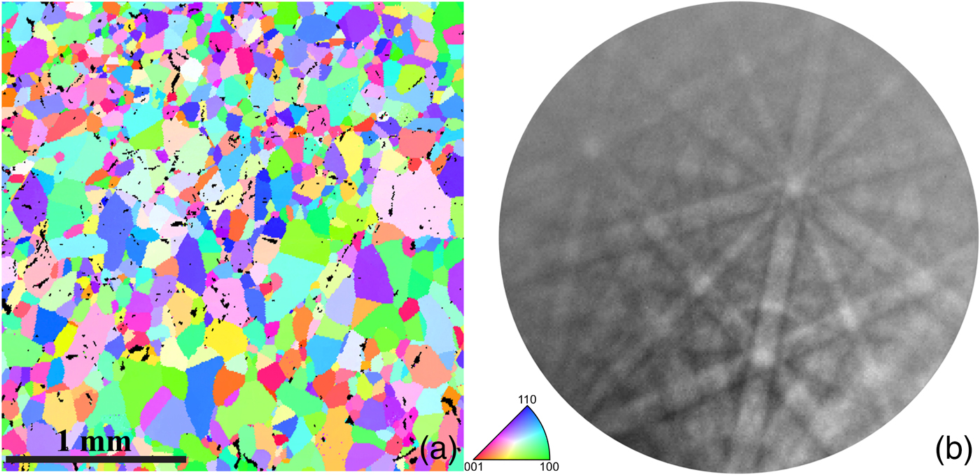
Fig. 2. (a) Orientation map for rutile sample showing the crystal direction aligned with the sample normal and (b) EBSD pattern of average quality from the rutile scan.
Table 3. Rutile Reflector Ranking Using the Beta Parameter; Kinematical and Hough-Averaged Results are Shown in the Last Two Columns.
Bold (hkl) indices indicate reflectors that are present in the vendor-supplied list.
In general, the average Hough-peak intensities follow the same trend as the beta parameters. However, the agreement is better for the experimental patterns than the simulated patterns. This is, in part, due to the fact that the Hough algorithms in EDAX's OIM software have been tuned toward finding bands in experimental patterns and have only recently been applied to dynamically simulated patterns. In these experiments, we have shown results for the Hough-peak intensities obtained using the default set of Hough parameters in commercial software for consistency. However, we have noticed some differences in the average Hough-peak intensities based on the choice of Hough parameters. While only cursorily explored, the Hough rankings will be affected by the choice of Hough parameters used. For example, the Hough transform (or more correctly the butterfly convolution mask) can be biased toward detecting narrow bands over wide bands. The β hkl identified the {111} reflector as a reflector that should be included in the structure file and the Hough-peak intensity results confirm this conclusion in both the simulated and experimental patterns. In addition, the Hough results will be affected by the frequency with which a given reflector appears in the patterns as well as where they appear in the pattern. The quality of signal varies across the pattern and the peaks deviate from the ideal “butterfly” shape (see Krieger Reference Krieger1992). The Hough is normalized to mitigate this effect, but there will be still some effect on the intensities of the measured peaks.
Forsterite
EBSD patterns were simulated for forsterite at uniformly sampled grid orientations covering all of orientation space (15, 903 in total); the patterns were simulated for the following pattern center coordinates: (x*, y*, z*) = (0.5, 0.5, 0.7) with a detector tilt of 10° and a sample tilt of 70°. These patterns were indexed using TSL OIM 8 software using the vendor provided structure factor (I hkl) ranking as well as the beta (β hkl) rankings shown in Table 4. Figure 3 shows the cumulative histogram of the simulated patterns as a function of the confidence index. The curve clearly shows the increase in the confidence index when using theβ hkl rankings; the median confidence index using the traditional I hkl rankings was equal to 0.15, while using the β hkl rankings for the indexing process boosted the median confidence index to about 0.35. In forsterite, the first 24 reflectors in the β hkl ranking were all included in the original vendor supplied structure file. Beyond the first 24 reflectors, the structure file also included the following reflectors: {921}, {741}, {660}, and {240} which were respectively ranked 25th, 31st, 34th, and 54th. This shows the value of the beta rankings as an operator would want to confirm the inclusion/exclusion of these lower ranking reflectors in the optimized list.
Fig. 3. Cumulative histogram of the confidence index with the fraction of indexed patterns for forsterite using the kinematical intensities (I hkl) and the β hkl rankings.
Table 4. Forsterite Reflector Ranking Using the Beta Parameter; Kinematical and Hough-Averaged Results are Shown in the Last Two Columns.
Bold (hkl) indices indicate reflectors that are present in the vendor-supplied list.
The three intensity profiles for forsterite are shown in Figure 4 as a function of the beta parameter ranking. Note that both β hkl and  $I_{hkl}^{{\rm HSP}} $ decrease until about rank 27, and then level off or oscillate around an average value of about 14; this indicates that there is likely not much to be gained from including these higher rank reflectors in the Hough-indexing process. The $I_{hkl}^{{\rm abs}} $ profile oscillates strongly over the entire range of ranks ([1…60]), reflecting the fact that the kinematical ranking for this crystal structure is quite different from the ranking derived from the beta parameters. Thus, beta parameter ranking will likely prove to be useful for the Hough-based indexing of EBSD patterns from more complex crystal structures.
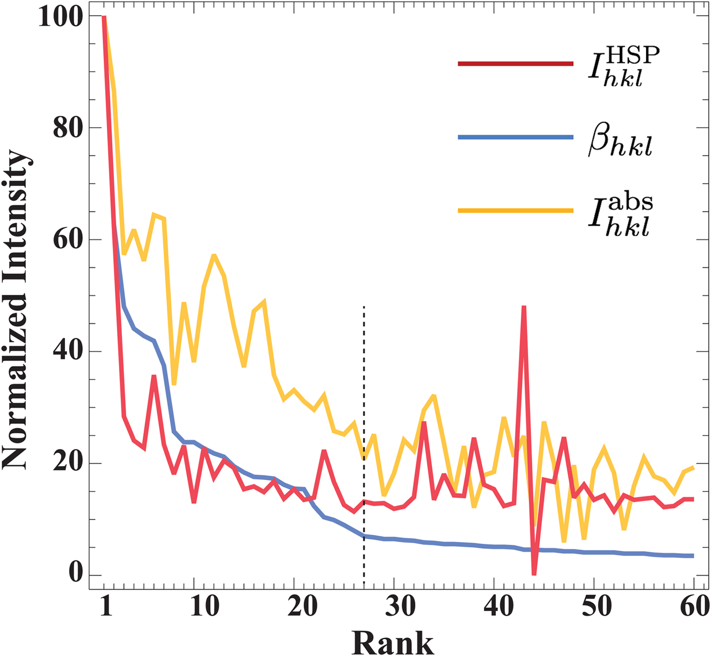
Fig. 4. Plot of the three normalized intensities (β hkl,  $I_{hkl}^{{\rm abs}} $, and $I_{hkl}^{{\rm HSP}} $) as a function of the beta rank. The vertical dashed line indicates where the β hkl and $I_{hkl}^{{\rm HSP}} $ curves start to level off.
Conclusions
For the elemental materials (Ni and Si), there is much better correlation between the  $I_{hkl}^{{\rm HSP}} $ ranking and the β hkl than between the $I_{hkl}^{{\rm HSP}} $ ranking and the $I_{hkl}^{{\rm abs}} $ rankings. In the more complex materials, the $I_{hkl}^{{\rm HSP}} $ and β hkl are not in as close an agreement as in the elementary structures, but they do follow the same general trends—the $I_{hkl}^{{\rm HSP}} $ results tend to be noisier. Nonetheless, the β hkl results for the more complex materials identified some relatively strong reflectors that should be included in the reflector list. For example, {111} in rutile and {331} in forsterite which in both cases were confirmed by Hough results on simulated patterns as well as on experimental patterns in the case of rutile.
In all cases, the results show that the beta parameter provides a much better starting point for optimizing the list of reflectors used in Hough-transform-based indexing over the kinematical ranking. The β hkl ranking can be coupled with a set of simulated patterns to not only further optimize the list of reflectors but also to provide guidance on the parameters used for peak detection via the Hough transform.
The algorithms for the computation of the EBSD master pattern and the reflector ranking described in this paper are available as open source code from the following Git Hub repository: http://github.com/EMsoft-org/EMsoft.
Author ORCIDs
Marc De Graef, 0000-0002-4721-6226
Acknowledgments
The authors gratefully acknowledge Gregory S. Rohrer of Carnegie Mellon University for supplying the rutile sample. SS and MDG would like to acknowledge a DoD Vannevar-Bush Faculty Fellowship (no. N00014-16-1-2821). The work of SS was performed partially under the auspices of the U.S. Department of Energy at Lawrence Livermore National Laboratory under Contract DE-AC52-07NA27344 (LLNL-JRNL-762497). All authors wish to acknowledge the computational facilities of the Materials Characterization Facility at CMU under grant # MCF-677785.


