


Introduction
The characterization of distributed particle properties is a key challenge in chemical engineering to understand the relation between microscopic features and macroscopic effects. Two-dimensional (2D) imaging methods are used to reveal multiple properties at once. Static methods, such as light microscopy, were supplemented by dynamic methods, which represent a significant development, especially with regard to the statistical representativeness of the samples (Brown et al., Reference Brown, Vickers, Collier and Reynolds2005). Image tracking algorithms were used to compensate for stereological errors from the 2D image description, but only down to particle sizes of around 100 μm (Macho et al., Reference Macho, Kabát, Gabrišová, Peciar, Juriga, Fekete, Galbavá, Blaško and Peciar2019). A complete three-dimensional (3D) description of a collective of particles smaller than 10 μm is not possible with these methods.
Computed tomography (CT) measuring methods, on the other hand, are well-established over length scales from centimeter to the submicrometer range. Depending on the physical measurement principles and the experimental setup, every measuring method has its limitations, both in analysis volume and spatial resolution. X-ray CT is one of the most common 3D imaging techniques used in the engineering sciences to visualize internal structures of solid-state phases nondestructively (Stock, Reference Stock1999). The X-rays used are capable of penetrating solid matter, their absorption coefficient being a function of the material density of the sample, the length penetrated, the photon energy, and the atomic number of the compound elements. The measurement parameters are therefore strongly related to the material and its dimensions (Pavlinsky, Reference Pavlinsky2008). Compared to 2D radiological imaging, the tomography setup offers a chance to analyze the 3D structure of objects in the field of view (FOV) without stereological error. By rotating the sample, a series of projections can be captured—each image with the attenuated sum signal along the beam path. The transformation of the series of 2D images into a 3D volume is based on Fourier, algebraic, or statistical algorithms (Buzug, Reference Buzug2008).
Initially only available at monochromatic synchrotron facilities, state-of-the-art systems are now also available in laboratories, for micrometer (X-ray micro-computed tomography, micro-CT) and submicrometer range imaging (X-ray nano-computed tomography, nano-CT) (Maire & Withers, Reference Maire and Withers2014). This has opened up the possibility to work on extensive questions from particle measurement technology even without access to measurement time at synchrotron beamlines.
Particles with sizes below the voxel resolution are often used for contrast enhancement of complete phases or as markers of specific regions (Shilo et al., Reference Shilo, Reuveni, Motiei and Popovtzer2012). Alternatively, particles with sizes larger than the voxel resolution can be used directly as alignment markers in 3D imaging (Hagen et al., Reference Hagen, Werner, Carregal-Romero, Malhas, Klupp, Guttmann, Rehbein, Henzler, Mettenleiter, Vaux, Parak, Schneider and Grünewald2014). Studies on particle properties can be found for single particles (Liu et al., Reference Liu, Meirer, Krest, Webb and Weckhuysen2016), a limited number (10–100) of free particles (Bagheri et al., Reference Bagheri, Bonadonna, Manzella and Vonlanthen2015), as crystals in mineralogical phases (Kahl et al., Reference Kahl, Dilissen, Hidas, Garrido, López-Sánchez-Vizcaíno and Román-Alpiste2017) or as macroscopic units with properties like layer thickness (Zhong et al., Reference Zhong, Burke, Withers, Zhang, Zhou, Burnett, Liu, Lyon and Gibbon2019) or bulk properties (Sjödahl et al., Reference Sjödahl, Siviour and Forsberg2012). In contrast, the tomographic analysis of particulate samples of a statistically relevant quantity (more than 1000 particles) with distributed multidimensional properties is rarely mentioned in the literature (Cepuritis et al., Reference Cepuritis, Garboczi, Jacobsen and Snyder2017).
Since particle systems are, in many cases, composed of particles with size distributions covering more than one size scale, a multiscale approach is a fundamental requirement in order to be able to describe them precisely with respect to their multidimensional properties. Studies often focus on solids to determine material properties like layer composition (Moroni et al., Reference Moroni, Börner, Zielke, Schroeder, Nowak, Winter, Manke, Zengerle and Thiele2016) or micro-processes like crack formation (Burnett et al., Reference Burnett, McDonald, Gholinia, Geurts, Janus, Slater, Haigh, Ornek, Almuaili, Engelberg, Thompson and Withers2014). In this study, we investigated a mixture of two particle systems of very different particle sizes. We created a 50/50 (by weight) mixture of spherical glass particles (diameter min 0.4 μm, median 1.2 μm, max 5.8 μm) and glass fibers (diameter 10 μm, median length 82 μm, longest fiber 660 μm) to investigate a borderline case of maximum difference in the aspect ratio and a significant difference in size. Thus, the geometrical properties of spheres and fibers can only be analyzed simultaneously by a combination of tomographic analysis methods on two magnification levels (X-ray micro- and nano-CT).
The basis of a quantitative evaluation of the reconstructed tomography image data is a sequence of individual image processing algorithms that is precisely adapted to the properties of the individual particles in the image (image processing workflow). In our case, we start to identify the fibers and the spheres by segmentation. This is a fundamental step, since the statistical analysis of the particle system strongly depends on the shape and size of the particles and thus on the quality of segmentation. Therefore, we apply the so-called marker-controlled watershed transform, one of the most widely used segmentation algorithms, which has proved to be robust and efficient (Meyer & Beucher, Reference Meyer and Beucher1990; Soille, Reference Soille2013). The geometry of a segmented fiber is characterized by its length, specific surface area, and cross-section diameter. A parametric representation of the bivariate distribution of the fiber's length and the specific surface area is obtained using copula theory (Durante & Sempi, Reference Durante and Sempi2015). The fitted copula model enables to capture the correlation structure between the length and the specific surface area (the so-called marginal distributions), hence, leading to a more informative description of the fiber system. For the spheres, the volume-equivalent diameter and the specific surface area are used as geometrical criteria, and a copula model is also fitted to this bivariate distribution. Therefore, it is possible to get a full parametric description of the entire particle system by combining the two individual copula models, either using a number- or volume-weighted version of the bivariate probability density functions.
This paper is organized as follows. In the section Materials and Methods, we introduce our sample preparation method, focusing on representativeness and sample size. A summary of the measurement parameters and the description of the image processing procedure then presented. In the section Results and Discussion, we propose a reasonable multidimensional characterization approach, using a copula model and correcting edge effects, to characterize the particulate material composed of fibers and spheres.
Materials and Methods
Preparation of Particulate Samples
A conclusive tomographic analysis of a particulate sample has to meet the following requirements:
1. Enough particles to describe statistically relevant distributed properties.
2. FOV-adjusted sample size to avoid large scanning times and artifacts.
3. Spatially separated particles to avoid segmentation errors.
4. An appropriate voxel size to distinguish interesting features.
These four requirements have to be balanced with respect to the number and the size ranges of particles. The last two requirements are related to the partial volume effect (see Supplementary Appendix B).
Statistical Representativeness
Analyzing particles as a collective with distributed properties requires a representative sample within a scanned volume. Practical approaches to calculate a minimum number of particles based on statistical models are given in the literature (Koglin et al., Reference Koglin, Leschonski and Alex1974; Vigneau et al., Reference Vigneau, Loisel, Devaux and Cantoni2000). We determined the optimal volume concentration of spherical particles, immobilized and embedded in a matrix, in prestudies with 10 vol% (Ditscherlein et al., Reference Ditscherlein, Leißner and Peuker2019). The minimum concentration c min is given by the ratio of the total particle volume V Particle and the volume of the sample cylinder V Cylinder, i.e.,
 $$c_{{\rm min}} = {V_{{\rm Particle}}\over V_{{\rm Cylinder}}} = {n_{{\rm Particle}}\cdot{4 \over 3}\pi\cdot x^{3}\over n_{{\rm Stitch}}\cdot\pi\left({d_{{\rm C}} \over 2}\right)^{2}\cdot h_{{\rm C}}},$$
with the number of particles n Particle, equivalent spherical particle diameter x, the number of vertical stitches n Stitch (in this study, equal to 1), diameter d C, and height h C of the sample cylinder. In Figure 1, the determined minimum number of particles is shown as a set of ISO-lines going from low particle volume concentrations to a limit concentration for a monodisperse particle fraction (hexagonal close packing, c ≈ 0.74, see case (b) in Fig. 1). Due to limited machining capabilities for sample preparation, there is also a practical lower limit of the sample size (c). The shift from a large FOV (a-1) to a smaller one (a-2) with constant particle size (equivalent spherical diameter) means that the resulting operating point is near the first ISO-line (10,000 particles) for c min = 0.01. The estimation of the minimum concentration using equation (1) is exact solely in the case of sphere-like particles. The generation of a sufficient fiber statistic is much more challenging when combined with spheres which are two to three scales smaller than the longest fiber. In such a situation, the measurement of a suitable sample volume over two different length scales is required.

Fig. 1. Possible working area for preparation of particulate samples for a target particle number of 10,000 going from large FOV (a-1) to a smaller FOV (a-2), with concentration limit for spherical monodisperse hexagonal close packing (b) and a minimum FOV due to sample processing (c).
Sample Size Adjustment
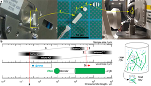
If the required FOV at a chosen magnification is smaller than the biggest lateral dimension of the sample, regions that are only illuminated by penetrating X-rays in certain angle ranges create artifacts in the reconstructed sample volume (Kyrieleis et al., Reference Kyrieleis, Titarenko, Ibison, Connolley and Withers2010) (especially for highly X-ray absorbing materials). A well-known rule of thumb to determine the needed number of tomographic projections is n Projection = π/2 · n Pixel,Detector. For scans inside the sample (Region of interest tomography, see Supplementary Appendix D), the detector does not cover the entire area of the actual projection image that can lead to artifacts in the final reconstruction. To avoid that, the number of detector pixels n Pixel,Detector has to be increased to reach the largest lateral dimension of the sample (n Pixel,Sample). This requires a much longer scan time, not only by increasing the number of projection angles but also by the longer X-ray radiation per projection angle. In the case of monochromatic X-rays (nano-CT), the integral energy flux is very low compared with the polychromatic radiation of the micro-CT (for details regarding the CT scanners, see Section Multiscale tomographic measurement or Supplementary Appendix C). Thus, these effects are getting even worse. Reducing sample size (Fig. 2a) is the best way to minimize scan time and to avoid artifacts. Nevertheless, a system of particles with very high aspect ratio (fibers) is a natural limitation. This can only be overcome by measuring on two different scales with two different sample sizes: Large samples for low-resolution (low-res) scans and smaller samples for medium-resolution (med-res) and high-resolution (high-res) scans.

Fig. 2. Large sample mounted on rotating sample stage (a-1), unmounted (a-2) for slicing in small disks (a-3) and sectioning into a small bar (a-4), and remounted for medium- and high-resolution measurements (a-5). Relation between sample size, voxel size, and characteristic particle size—corresponding range marked with a box: extended FOV of nano-CT by ROI measurement (b-1), minimum sample size limited by machining (b-2), fixed correlation between sample and voxel size determined by binning factor (b-3), overlapping measurement field for determining fine particle fraction (b-4), and micro-CT measurement to determine fiber length (b-5).
Immobilization by Wax Embedding
The particle system considered in this study was a mixture (50/50 by weight) of two types of glass particle fractions, one being spheres and the other fibers. Spherical soda-lime glass particles were purchased from VELOX, Germany (SG7010, Q 0.10 0.62 μm, Q 0.50 2.67 μm, Q 0.90 4.99 μm), borosilicate-glass fibers from Schwarzwälder Textil-Werke, Germany (FG160/060) with median fiber length of 82 μm, largest fiber length of 660 μm, and narrowly distributed average fiber diameter of 10 μm. Some statistical measures were performed using images acquired from light microscopy and scanning electron microscopy (SEM) and are summarized in Supplementary Appendix A.
To avoid motion artifacts and to ensure the spatial homogeneity of the particles in a sample volume for optimal image segmentation results, the particles must be immobilized. Conventional methods of particle embedding in epoxy-based resins, as used in the preparation of polished sections, e.g., multidimensional particle analysis using Mineral Liberation Analysis (MLA) (an example given by Buchmann et al., Reference Buchmann, Schach, Tolosana-Delgado, Leißner, Astoveza, Kern, Möckel, Ebert, Rudolph, van den Boogaart and Peuker2018), are not suitable here due to the long curing times. Therefore, we have embedded the particles in a histological wax that is normally used for biological sample preparation. We used a target volume concentration of 10%, which we controlled in image segmentation afterwards. Subsequent to drawing of the molten wax particle suspension into a polymer tube, the volume was shock-frozen within the small polymeric tube, resulting in a sample cylinder of approximately 1.6 mm diameter after forming (Ditscherlein et al., Reference Ditscherlein, Leißner and Peuker2020). Figure 2a shows the sample preparation procedure beginning with a cylindrical shape (2 mm diameter, a-1) for low-resolution scans, that is manually sliced down (a-3 and a-4) to a bar for medium- and high-resolution scans (≈0.5 mm diameter, a-5). In previous studies (Ditscherlein et al., Reference Ditscherlein, Leißner and Peuker2019), we showed that the particles are homogeneously distributed over the sample height. Thus, considering two of these different positions from the cylindrical sample was sufficient for the current study.
Multiscale Tomographic Measurements
When handling voxel-based data, it is important to distinguish between voxel and spatial resolution. The voxel resolution only describes the 3D equivalent to the detector pixel resolution (considering the binning to virtual pixels), which is given by the mechanical and optical magnification of the system. This information is insufficient with respect to the effective spatial (structural) resolution, which is a function of the measurement parameters and the properties of the sample itself. Taking this into account, objects smaller than 100 voxels were removed from the data set. In all three resolution modes, the tomograms were exported as a stack of tiff images of approximately 1024 × 1024 pixels. A comparison of both experimental setups is shown in Supplementary Appendix C. Measurement parameters are summarized in Table 1.
Table 1. Measurement and Reconstruction Parameters of All Three Resolution Modes—Low-Resolution (low-res), Medium-Resolution (med-res), and High-Resolution (high-res).

* denotes not applicable for monochromatic measurements.
Micro-CT Measurements
Low-resolution and medium-resolution measurements were performed using a micro-CT (Zeiss Xradia VERSA 510) with a polychromatic X-ray source, a rotating tungsten anode, a maximum acceleration voltage of 160 keV, and a maximum power of 10 W. Compared to conventional X-ray micro-CT systems, an additional optical system increases magnification by a factor of 10. This two-step magnification gives a minimum voxel size of 0.3 μm. Reconstruction was done using the software Zeiss XMReconstructor (Version 11.1.8043) with the aim of minimizing manipulations in preprocessing (smoothing, beam-hardening correction). No beam hardening was visible in the reconstructed slices. Due to the cone beam artifact, 50 slices were removed from the top and bottom of the data set before image postprocessing. A summary of relevant artifacts related to micro-CT measurements is given by Boas & Fleischmann (Reference Boas and Fleischmann2012) and Davis & Elliott (Reference Davis and Elliott2006).
Nano-CT Measurements
High-resolution imaging was performed using a nano-CT (Zeiss Xradia Ultra 810), which operates at a constant X-ray photon energy of 5.4 keV (monochromatic, no beam-hardening artifacts) with parallel beam geometry (no cone-beam artifacts) and a rotating chromium anode. The minimum voxel size in high-resolution mode is 16 nm. For the experiments, absorption contrast imaging in large field of view mode (minimum voxel size 64 nm) was used. Image reconstruction was performed by means of the software Zeiss XMReconstructor (Version 10.0.3878.16108).
Image Segmentation
Marker-Controlled Watershed Transform
The segmentation procedure for each CT image is based on the marker-controlled watershed transform. One of the first papers where the watershed transform was considered is presented by Meyer & Beucher (Reference Meyer and Beucher1990). It takes advantage of the topographic representation of a grayscale image: the parts of the image with low intensities are represented as “valleys,” while the regions with high intensities are assimilated as high altitude reliefs. First, a set of regional minima M of the image has to be determined. Then, the construction of the watershed lines can be seen as the result of a flooding process: water starts to rise at a constant speed from the minima and a dam is constructed if two or more floods from different minima may touch. The resulting dams are the watershed lines and delimit the segmented regions (called catchment basins) of the images. For further details on the watershed transform, see Soille (Reference Soille2013), Vincent & Soille (Reference Vincent and Soille1991), and Gonzalez et al. (Reference Gonzalez, Woods and Eddins2002).
The marker-controlled watershed transform is an adaptation of the classical watershed transform for which the set of minima M is considered as a set of markers. Each marker locates an individual object to be segmented. The ridge lines will then be the contours of the objects. In general, the set M of markers may be difficult to construct. The construction of the markers depends usually on the type of the image and the object properties (shape, size, gradient intensity, etc.).
Segmentation of Low- and Medium-Resolution CT Images
For the low spatial resolution (low-res) CT image, only the fibers are clearly visible. Thus, the segmentation procedure consists of the following main steps:
1. Global thresholding and morphological opening operation to remove small objects.
2. Computation of Euclidean distance transform of the complemented binary image of the fibers.
3. Marker computation: extended-maxima transform of the distance transformation computed in step 2.
4. Application of the marker-controlled watershed transform.
In steps 1 and 2, rather basic image processing operations are performed (Serra, Reference Serra1983; Gonzalez et al., Reference Gonzalez, Woods and Eddins2002). Step 3 is a well-known technique (Soille, Reference Soille2013) to construct a set of markers from the Euclidean distance transform, and step 4 is the application of the marker-controlled watershed transform using these markers (Soille, Reference Soille2013). The flowchart in Figure 3 illustrates the application of these steps for a specific slice. Further segmentation results are visualized in Figure 4. The fibers (in blue) are generally well segmented. However, some under segmentation is observed. It is addressed with a postprocessing procedure (described below).

Fig. 3. Segmentation procedure for the CT images. The red arrows correspond to the input and output of the segmentation procedure. The green arrows provide the intermediate results for each of the transformations.

Fig. 4. Examples of segmentation results for each resolution on different slices (a). The boundary of each segmented particles is highlighted in blue. Examples of removed objects (in green) after the postprocessing procedure (b).
The segmentation of spherical particles for the medium spatial resolution (med-res) CT image is a challenging task as the particles are too small to be clearly visible. After having removed the fibers from the image, the proposed segmentation procedure is the same as for the low-res CT image. The spheres (in blue) are generally highly under-segmented. Indeed, noise and artifacts especially affect the binarization of small objects (for details regarding the partial volume effect, see Supplementary Appendix B).
Segmentation of High-Resolution CT Image
The segmentation procedure for the high spatial resolution (high-res) CT image consists of the following main steps:
1. Intensity adjustment and smoothing with a nonlocal mean filter (using a Gaussian kernel).
2. Performing a morphological ultimate opening operation.
3. Global thresholding. The binary image is further cleaned up with a morphological opening operation: small objects of less than 100 voxels are removed.
4. Computation of Euclidean distance transform of the complemented binary image.
5. Marker computation using the extended-maxima transform.
6. Application of the marker-controlled watershed transform.
Figure 3 illustrates the application of these steps for a specific slice. Steps 1 and 3–6 have already been detailed for the segmentation of the low-res CT image. The ultimate morphological opening (Beucher, Reference Beucher2005, Reference Beucher2007) (step 2) is a less-known technique for image segmentation. Note that the ultimate opening operator θ(v) is defined as follows:
 $$\theta\lpar v\rpar = \sup_{i \in \lcub 1\comma \ldots\comma N\rcub }\lpar \psi_i\lpar v\rpar -\psi_{i + 1}\lpar v\rpar \rpar \quad \hbox{\,for each } v \in V\comma $$
where V is the set of voxels, N is some integer, and ψi, respectively ψi+1, is the morphological opening operator for a closed ball of radius i, respectively i + 1. Then, the voxel intensity values of the resulting image are the largest differences between the voxel intensity values of successive openings. An important consequence is that spherical objects, having the same textural information, are emphasized. Therefore, the binarization of a union of sphere-like particles is easier to undertake after preprocessing the image with the ultimate opening operation. Note that the value of N should be larger than the radius of the biggest sphere within the image. Hence, the main drawback of the ultimate opening is the computation time required to perform openings for balls of important radii. Other applications of the morphological ultimate opening were considered for text detection (Retornaz & Marcotegui, Reference Retornaz and Marcotegui2007), for facade segmentation (Hernandez & Marcotegui, Reference Hernandez and Marcotegui2008), and for detection of microaneurysms on eye fundus images (Zhang et al., Reference Zhang, Thibault and Decencière2011).
Postprocessing of Segmented Images
A postprocessing procedure is applied to remove bias due to under or over segmentation. Regarding the segmentation of fibers in the low-res CT image, the following convexity constraint for a segmented object S should be satisfied:
 $${\#S\over \#{\rm Conv}\lpar S\rpar } \geq 0.5\comma\; $$
where #S is the number of voxels of S and #Conv(S) is the number of voxels of its convex hull. The topological constraint in equation (3) allows the reduction of the bias due to under segmentation, resulting in nonconvex objects (see Fig. 4b).
For the spherical particles, a constraint on the shape of the segmented objects is used. The sphericity coefficient Ψ, defined as the ratio of the surface area of the volume-equivalent sphere divided by the surface area of the corresponding segmented object, quantifies the deviation from the spherical shape (Wadell, Reference Wadell1932; Bailey et al., Reference Bailey, Gomez and Finch2005; Lau et al., Reference Lau, Deen and Kuipers2013). Note that for a segmented object S, its sphericity ΨS is given by
 $$\Psi_S = {\pi^{1/3}\lpar 6V_S\rpar ^{2/3}\over S_S}\comma\; $$
where V S and S S are the volume and the surface area of S, respectively. The closer ΨS is to 1, the closer the shape of the segmented object S is to that of a sphere. A standard estimator of V S is the number of voxels of the segmented object S. The estimator used for the surface area S S of S is based on the Crofton formula of integral geometry (Schneider & Weil, Reference Schneider and Weil2008). A formal definition of the estimator can be found in Schladitz et al. (Reference Schladitz, Ohser and Nagel2006). Thus, all particles whose sphericity coefficient is smaller than the threshold of 0.8 and 0.45 for the high-res and med-res CT image, respectively, are removed. The values of these thresholds were fixed empirically by visual inspection.
Results and Discussion
Correction of Edge Effects
A common problem encountered in spatial statistics is that of edge effects. They occur when the estimation of a certain geometrical characteristic requires information from outside of the sampling window. For instance, when determining the lengths of a population of fibers within an image, all fibers that cut the boundary of the sampling window are only partially observed. Taking into consideration only the fully observed fibers leads to a length distribution which is biased because the probability that a long fiber intersects the boundary of the sampling window is higher than the one of a short fiber. In our case, the minus-sampling method (Ohser & Schladitz, Reference Ohser and Schladitz2009; Chiu et al., Reference Chiu, Stoyan, Kendall and Mecke2013) is used, which consists of taking a sub-window contained in the sampling window such that all particles with nonempty intersection with the sub-window are completely observed in the entire sampling window. Then, considering all particles such that their center of mass is inside the sub-window leads to an unbiased sample of the population of particles.
An illustration how the minus-sampling method is applied in the case of fibers is provided in Figure 5. The gray area visualizes a cross section through the cylindrical sampling window. The sub-window is the cylinder, whose cross section is delimited by the red circle. All fibers in the sub-window do not intersect the boundary of the entire sampling window. Then, only the fibers (in blue in Fig. 5) whose center of mass is inside the sub-window are considered for the statistical analysis. The fibers highlighted in red are removed by the minus-sampling technique. Note that the minus-sampling technique cannot be used if the sub-window does not include a sufficiently high number of fibers. Analogously, the minus-sampling technique is applied to image data from which the spherical particles are extracted. After applying the minus-sampling method, the remaining segmented particles are the basis for an efficient characterization of the particulate sample, using parametric bivariate distributions of particle properties. First, we fit such distributions to particle properties of spherical particles and fibers individually. Then, the distributions for the individual fractions have been combined to obtain a distribution characterizing the entire sample.

Fig. 5. Minus-sampling technique to remove bias due to edge effects. The red circle is a cross section of the minus-sampling window, i.e., only particles whose centroid is inside this reduced sampling window are sampled. Furthermore, the particles highlighted in red are removed. The particles in green are removed due to the postprocessing technique. Only blue particles are taken into account for the statistical analysis.
Multidimensional Characterization of Spherical Particles
Univariate Distributions of Particle Size and Specific Surface Area
For each spherical particle, the size d and the specific surface area  $S_{V_p}$ are computed as geometrical characteristics. In the case of spherical particles, the size d equals the volume-equivalent diameter $d_{{\rm eq}\comma V_p}$ which is given by
 $$d_{{\rm eq}\comma V_p} = \left({6V_p\over \pi}\right)^{1/3}\comma\; $$
where V p is the volume of the segmented sphere. The volume V p is computed by counting the voxels belonging to the particle followed by scaling with a single voxel's volume. Since the spherical particles are not perfect spheres their surface area S cannot be directly computed from their size  $d_{{\rm eq}\comma V_p}$. Therefore, we compute the surface area directly from image data using the Crofton formula (Lehmann & Legland, Reference Lehmann and Legland2012). Then, the specific surface area $S_{V_p}$ is given by
 $$S_{V_p} = {S\over V_p}.$$
Supplementary Figure S2 provides histograms of the particle size d for two resolutions. The significant differences between the distributions in the med-res and high-res CT images are not surprising. For the med-res CT images, important under segmentation, due to blurred small spheres or noise/artifacts, was observed. Hence, the distribution is biased toward larger sphere sizes. Moreover, very small spheres, whose volume-equivalent diameters are less than 1.5 μm, are not detected due to the insufficient resolution of the med-res CT images. In contrast to this, a large fraction of spheres in the nanometer range is correctly segmented and analyzed in the high-res CT images. The high resolution also enables us to overcome the under segmentation problem encountered for the med-res CT images. Consequently, the particle size distribution is right-skewed (see Fig. 6a). Thus, for the analysis of the spherical particles, from hereon, we will solely use two high-res images depicting the spherical particles at spatially different locations. Histograms of the spherical particle's size and specific surface area computed from these images are visualized in Figure 6a.

Fig. 6. Statistical analysis of the segmentation results. Fitted parametric (marginal) distributions to size (left) and specific surface area (right) of the spherical particles (a); bivariate histogram (left) and its copula model (right) (b); number-weighted (left) and volume-weighted (right) bivariate probability density of size and specific surface area of the entire particle system (c). Note that the number-weighted visualization has a logarithmically scaled colorbar.
For validation purposes, we compared the particle size distributions computed from high-res image data and the SEM images (see Fig. 7). The method to derive the particle size distribution from the SEM images is explained in Supplementary Appendix A. We observe an underestimation of the relative frequency for particles with a diameter smaller than 0.6 μm in the case of the high-res CT images. This is mainly due to the higher resolution of the SEM images, which allows one to distinguish smaller spheres more clearly. For the high-res CT images, with a resolution that is two times lower, it is hardly possible to segment such small-sized spheres due to noise and artifacts. For bigger particles, the two distributions are consistent, which demonstrates the possibility of using the nano-CT imaging technique in this size range. Note that some overlapping effects appear in the SEM images (see Supplementary Appendix A), which may complicate the segmentation process and bias the volume-equivalent diameter distribution. Besides, the volume fraction of the segmented spheres in one of the high-res images is about 4.4% (sample 1), which is slightly smaller than the expected volume fraction of 5% (see Section Material and Methods). In the other high-res image, the volume fraction of 2.6% deviates significantly more from the target value. The reason for this is the extremely small FOV of the high-res measurement and the nonhomogeneous distribution of the population of spheres within the sample volume. Since this effect is independent of the particle size, the particle size distribution remains unaffected.

Fig. 7. Comparison of the size distributions computed from the CT images (in blue) and the SEM and light microscopy (in red) images.
Copula Approach
Since univariate histograms of one-dimensional particle characteristics do not provide information about the correlation between the considered characteristics, a more informative description of the particulate system of spheres can be achieved by investigating bivariate distributions. For this purpose, a parametric model can be used to characterize the joint distribution of size d and specific surface area  $S_{V_p}$ of the spherical particles. Note that the distribution of d (see Fig. 6a) is clearly not Gaussian, yet the values of d and $S_{V_p}$ are strongly correlated with a correlation coefficient of − 0.89. Thus, standard methods, which approximate the joint distribution of size d and specific surface area $S_{V_p}$ with a product distribution or a bivariate Gaussian distribution, are not applicable in our case. Therefore, the joint distribution will be modeled using copula theory (Durante & Sempi, Reference Durante and Sempi2015).
Note that a 2D copula C : [0,1] 2 → [0,1] is a cumulative distribution function whose marginal distributions are uniform on the unit interval [0,1]. It enables us to characterize the dependency between correlated non-normally distributed random variables. Specifically, in the 2D case, Sklar's theorem (Durante & Sempi, Reference Durante and Sempi2015) states that, given two real-valued random variables X 1 and X 2 with cumulative distribution functions F 1 and F 2, there exists a copula C such that the joint cumulative distribution function F of X 1 and X 2 is given by
 $$F\lpar x_1\comma x_2\rpar = C\lpar F_1\lpar x_1\rpar \comma F_2\lpar x_2\rpar \rpar \comma\; \quad \hbox{\,for each } \lpar x_1\comma x_2\rpar \in {\mathbb{R}}^2\comma $$
where  $F\lpar x_1\comma x_2\rpar = {\mathbb P}\lpar X_1\le x_1\comma X_2\le x_2\rpar$. From an easy computation, provided that C, F 1, and F 2 are differentiable, we find that the joint density f of X 1 and X 2 is given by
 $$f\lpar x_1\comma x_2\rpar = c\lpar F_1\lpar x_1\rpar \comma F_n\lpar x_2\rpar \rpar f_1\lpar x_1\rpar f_2\lpar x_2\rpar \comma \quad \hbox{\,for each } \lpar x_1\comma x_2\rpar \in {\mathbb R}^2\comma $$
where f 1 and f 2 are the marginal densities, and the function c is the probability density function of the copula, i.e.,
 $$c\lpar u_1\comma u_2\rpar = {\partial^2\over \partial u_1\partial u_2}\, C\lpar u_1\comma \comma u_2\rpar \comma \quad \hbox{\,for each } \lpar u_1\comma u_2\rpar \in \lsqb 0\comma 1\rsqb ^2.$$
Model Fitting
In order to fit a bivariate probability density f to the observed pairs of size and specific surface area, we first fit the univariate marginal densities f 1 and f 2. We considered eight possible choices of parametric unimodal distributions, namely the gamma, normal, log-normal, Weibull, generalized extreme value, Rayleigh, Nakagami, and Rician distributions. For each marginal, the best fit is the one with the lowest value resulting from the Akaike information criterion (Akaike, Reference Akaike1998) (AIC). Note that the AIC is a measure of goodness-of-fit which is defined by
 $${\rm AIC} = 2k-2\log\lpar L\rpar \comma $$
where k is the number of model parameters and L the maximum value of the likelihood function. The best fits were obtained for the inverse Gaussian distribution and the gamma distribution for the size and specific surface area of spherical particles, respectively (see Fig. 6a).
Now, in view of equation (8), the bivariate density f can be fitted by determining a suitable copula density c. Similarly to the univariate case, there are various parametric families of copulas whose parameters can be determined using the maximum likelihood method. More precisely, the bivariate density f was fitted by determining the optimal copula density c from a family of commonly used Archimedean copulas (Durante & Sempi, Reference Durante and Sempi2015), where the considered Archimedean copulas were the Ali-Mikhail-Haq, Clayton, Frank, Gumbel, Joe, BB1, BB3, BB5, and BB8 copulas (Durante & Sempi, Reference Durante and Sempi2015). The best fit, denoted by f sphere, which is the one with the highest maximum likelihood, was obtained for the BB1 copula (see Fig. 6b (right)).
Multidimensional Characterization of Fibers
For each fiber, the size d and the specific surface area  $S_{V_p}$ are computed. While the latter is determined in the same manner as for the spherical particles using equation (6), the size d of a fiber is estimated in a different manner. Namely, the size d is the number of voxels along the main directions of the segmented fibers, where a principal component analysis (Pearson, Reference Pearson1901) is used to determine the main direction of a given segmented fiber. Furthermore, for a fiber F, the diameter d cross of its cross section is estimated as the diameter $d_{{\rm eq}\comma A_F}$ of the area-equivalent disk which is given by
 $$d_{{\rm eq}\comma A_F} = \sqrt{{4 A_F\over \pi}}\comma $$
where A F is the area of the cross-section orthogonal to the main axis of the fiber and located at half of the fibers length. Histograms of the size, the specific surface area, and the diameter are provided in Supplementary Figure S7a. We observe that the fiber diameter distribution is concentrated around 10 μm with a low standard deviation of 1.1 μm, which is consistent with the provider specifications (see Section Materials and Methods). Moreover, we compared the size distributions obtained from the CT image and the light microscopy images (see Fig. 7). The two distributions are consistent, which validates the proposed segmentation procedure for the CT image. Besides, we obtained the following quantiles for the size distribution using the CT image: Q 0.10 = 35 μm, Q 0.50 = 69 μm, and Q 0.90 = 197 μm. These values are slightly lower than the ones derived using light microscopy in the pre-characterization procedure (see Supplementary Appendix A). This deviation is mainly due to some small fibers which were missed during the manual segmentation of the light microscopy images, which then leads to a shift of the size distribution toward longer fibers. Regardless of this manual segmentation incorrectness, the overall size distribution derived from the low-res CT image is consistent with that one of the pre-characterization. Besides, the determined volume fraction of fibers of 4.7% is only slightly smaller than the expected 5% (see Section Materials and Methods).
Similarly, to the approach described in the section Model Fitting, the joint distribution of fiber size and specific surface area can be fitted using parametric copulas. In this manner, we determine the bivariate probability density f fiber, depicted in Supplementary Figure S7b.
Characterization of the Entire Particle System
In the previous sections, we have modeled the bivariate probability densities f sphere and f fiber of particle size and specific surface area for spherical particles and fibers, respectively. While the probability density f fiber was derived using the low-res CT image data, for the density f sphere characterizing the spheres the high-res image data of the same particle system was utilized. Now, we combine these probability densities to obtain a multidimensional, multiscale characterization of the entire particle system. More precisely, the bivariate probability density f system of size and specific surface area of the entire particle system is given by
 $$f_{{\rm system}} = \lambda f_{{\rm sphere}} + \lpar 1-\lambda\rpar f_{{\rm fiber}}\comma $$
where λ ∈ [0,1] is the (number-based) mixing ratio λ. Since we know that the considered particle mixture is a 50/50 mixture (by weight) of spherical particles and fibers, we can determine the mixing ratio. More precisely, the volume-equality of the fractions is described by
 $$\lambda \int_{0}^\infty \int_{0}^\infty f_{{\rm sphere}}\lpar d\comma s\rpar V_{{\rm sphere}}\lpar d\rpar {\rm d}d \, {\rm d}s = \lpar 1-\lambda\rpar \int_{0}^\infty \int_{0}^\infty f_{{\rm fiber}}\lpar d\comma s\rpar V_{{\rm fiber}}\lpar d\comma s\rpar {\rm d} d\, {\rm d}s\comma $$
where  $V_{{\rm sphere}}\lpar d\rpar = {\pi \over 6}d^3$ is the volume of a sphere with diameter d and V fiber(d,s) is the volume of a fiber with size d and specific surface area s (see Supplementary Appendix E). By solving equation (13) for λ, we obtain the theoretical mixing ratio λ = 0.9995. The resulting bivariate and bimodal density f system is depicted in Figure 6c (left). If no prior information is available, the mixing ratio λ can be estimated from image data by
 $$\lambda = {{ n_{{\rm sphere}} \over V_{{\rm sphere\comma Cyl}} } \over { n_{{\rm sphere}} \over V_{{\rm sphere\comma Cyl}} } + { n_{{\rm fiber}} \over V_{\rm fiber\comma Cyl} } }\comma $$
where n sphere is the number of spherical particles observed in the volume V sphere,Cyl and n fiber is the number of fibers observed in the volume V fiber,Cyl.
Note that the visualization of the number-weighted probability density f system in Figure 6c (left) utilizes, due to the different length scales of the particles, logarithmic axes. Furthermore, due to the relatively large mixing ratio λ, a logarithmically scaled colorbar is required to visualize the second mode corresponding to the fibers. A different representation using the so-called volume-weighted version f system,3 of the number-weighted density f system is given by
 $$f_{{\rm system\comma 3}}\lpar d\comma s\rpar = {1\over c}\Big(\lambda f_{{\rm sphere}}\lpar d\comma s\rpar V_{{\rm sphere}}\lpar d\rpar + \lpar 1-\lambda\rpar f_{{\rm fiber}}\lpar d\comma s\rpar V_{{\rm fiber}}\lpar d\comma s\rpar \Big)\comma $$
where c is a normalization constant. The volume-weighted probability density f system,3 depicted in Figure 6c (right) no longer requires a logarithmically scaled colorbar for visualization purposes.
Both the bivariate number- and volume-weighted probability densities of particle size and specific surface area are important for the characterization and analysis of particle systems. In particular, the first one is of interest when small particles have a significant influence on the distribution of properties of the overall system, e.g., when considering the active surface of a catalyzer material. On the other hand, the volume-weighted probability densities can be of interest when the characterization focuses on the mass of particles, e.g., when investigating the mass of a valuable material after some separation process has been completed.
Conclusions
The combination of micro- and nanotomographic X-ray imaging is a powerful tool for the determination of multidimensional particle properties in the micro- and submicrometer range, capable of bridging several orders of magnitude of particle size. We have shown how to create a sample with a statistically representative number of immobilized particles consisting of two very different particle populations by embedding them into a wax matrix. Furthermore, we emphasized the importance of adapting the sample size to the field of view in order to link X-ray tomography across different scales.
In contrast to the fibers, the size of the spherical particles is at the lower resolution limit of micro-CT. Thus, smaller spherical particles below the micrometer range are not detectable in the reconstructed CT images, hence, leading to a bias in the volume-equivalent diameter distribution. To minimize this well-known phenomenon of voxel size-dependent description of 3D objects, we first minimized the sample size, switched to a better resolution (nano-CT) and, finally, applied suitable image processing algorithms and statistical analysis to characterize the population of spheres. The distributions of the volume-equivalent diameter estimated from the nano-CT and micro-CT images were significantly different, thus, confirming the need to adapt the experiment and the statistical analysis to the size and shape of the particles contained in the same particle system.
The sample volume must be large enough compared to the typical particle size in order to contain a statistically relevant number of particles and to remove edge effects when determining the distributions of their geometrical properties. First, the correlation structure of particle size and specific surface area has been modeled separately for spheres and fibers, using copulas. The fitted copula models provide a complete parametric description of the population of spheres and fibers and are methodologically easily adaptable to more irregularly shaped particles. Finally, by combining these two parametric distributions, we obtained a multidimensional characterization of the entire particle system.
Our proposed workflow (including sample preparation, measurement, image processing, and image analysis) for multidimensional characterization of micro- and nanoscale particle systems is the starting point for the analyses of products from multidimensional separation processes and will be further discussed in forthcoming studies.
Data availability
Reconstructed TIFF-stacks for high-resolution, medium-resolution, and low-resolution measurements are stored within the scientific data repository of the universities TU Dresden and TU Bergakademie Freiberg with all relevant metadata (Ditscherlein & Martins de Souza e Silva, Reference Ditscherlein and Martins de Souza e Silva2019).
Supplementary material
To view supplementary material for this article, please visit https://doi.org/10.1017/S1431927620001737.
Acknowledgments
The authors thank the German Research Foundation (DFG) for supporting the project as part of the priority program SPP2045 (313858373), which is dealing with highly specific multidimensional separation of technical ultra-fine particle systems below 10 μm, the funding of the micro-CT (INST 267/129-1) as well as the nano-CT (WE 4051/21-1).


 Open access