


Introduction
Fluctuation electron microscopy (FEM) and related techniques have proven themselves as a powerful method to study disordered materials regarding their structure and dynamics at the nanoscale (Gibson & Treacy, Reference Gibson and Treacy1997; Treacy et al., Reference Treacy, Gibson, Fan, Paterson and McNulty2005; Gibson et al., Reference Gibson, Treacy, Sun and Zaluzec2010; Hwang & Voyles, Reference Hwang and Voyles2011; Zhang et al., Reference Zhang, Maldonis, Liu, Schroers and Voyles2018; Radić et al., Reference Radić, Hilke, Peterlechner, Posselt and Bracht2019). Upon illumination with a fine electron beam, a disordered material will exhibit local intensity variations in nanobeam diffraction patterns (NBDPs) at different positions (Voyles & Muller, Reference Voyles and Muller2002). These arise due to coherent diffraction from nanoscale ordered regions which are linked to medium-range order (MRO). Here, nanoscale ordered regions do not correspond to perfect nanocrystals but rather denote types of MRO such as paracrystals for amorphous silicon (Treacy et al., Reference Treacy, Gibson and Keblinski1998). The intensity fluctuations observed in the NBDPs are characterized by the normalized variance V(k, R) (Treacy & Gibson, Reference Treacy and Gibson1996) which is calculated by
 $$V\lpar k = \vert \vec{k}\vert \comma\; R\rpar = {\langle I\lpar \vec{k}\comma\; R\rpar ^{2}\rangle_{n\comma \phi}\over \langle I\lpar \vec{k}\comma\; R\rpar \rangle_{n\comma \phi}^{2}}-1,$$
where R denotes the STEM probe size, meaning the beam's full width at half maximum (FWHM) of intensity, and k is the magnitude of the scattering vector. The normalized variance is obtained by calculating the respective averaged intensity terms over n NBDPs according to the “Annular mean of variance image” method from Daulton et al. (Reference Daulton, Bondi and Kelton2010). Lastly, these images are azimuthally averaged, indicated by ϕ in the equation. The probe size for FEM is chosen such that it matches the extent of MRO in the material in order to maximize the intensity variations and by this V(k, R) (Treacy & Gibson, Reference Treacy and Gibson1996; Gibson & Treacy, Reference Gibson and Treacy1997). Performing FEM measurements at different probe sizes is called variable-resolution FEM (VR-FEM) and can be used to extract more information about the disordered structure (Gibson et al., Reference Gibson, Treacy and Voyles2000; Voyles & Muller, Reference Voyles and Muller2002; Treacy et al., Reference Treacy, Gibson, Fan, Paterson and McNulty2005).
The normalized variance curves are affected by the experimental conditions such as sample thickness and probe characteristics (Yi & Voyles, Reference Yi and Voyles2011; Li et al., Reference Li, Bogle and Abelson2014). The latter aspect is important as quantitative results can only be obtained if the beam fulfills certain criteria. For instance, probe coherence plays a major role in this regard (Yi et al., Reference Yi, Tiemeijer and Voyles2010), and it has been demonstrated that beams with the same nominal size but different coherence yield different normalized variance curves (Li et al., Reference Li, Bogle and Abelson2014). Probe coherence depends on the illumination and how the probe is formed. Yi et al. (Reference Yi, Tiemeijer and Voyles2010) have shown that coherence is linked to the source size of the beam. This source size depends on, for example, the spot number and beam current on FEI microscopes and was quantified with a fit to the recorded probe profile. Those dependencies have been obtained at a single semi-convergence angle α. If one desires to change the probe size, one generally has to change α or resort to defocus, which has been claimed as an ineffective mean to change the probe size (Gibson & Treacy, Reference Gibson and Treacy2009). In this work, we want to compare these two methods.
Another aspect that influences the data is selecting the optimal exposure time τ. It is known that V(k, R) decreases as the exposure time increases (e.g., Rezikyan et al., Reference Rezikyan, Jibben, Rock, Zhao, Koeck, Nemanich and Treacy2015b). At low exposure times, V(k, R) will exhibit a strong upwards curve due to insufficient signal-to-noise at larger scattering vectors. Increasing the exposure time will reduce this effect but the question arises: is there a reasonable limit? For recording and evaluating a single image, for instance, a high-resolution TEM image, the exposure time is well chosen once there is enough contrast such that discernible features are clearly visible. However, for statistical analyses of intensity variations between diffraction patters, there might exist an ideal exposure time τ 0 at which one obtains the experimentally ideal data. For τ < τ 0, noise will affect the result, while at τ > τ 0, the local statistical intensity fluctuations could be negatively affected due to aspects such as prolonged beam-sample interactions or sample drift.
In diffraction experiments, signal arises due to scattering events and is, thus, directly linked to the sample thickness and total electron dose, j tot. By the total electron dose, we define the total number of electrons that passed through the material during the acquisition time. A high j tot leads to more beam-sample interactions which may be responsible for displacement decoherence that reduces the normalized variance (Reference Rezikyan, Jibben, Rock, Zhao, Koeck, Nemanich and TreacyRezikyan et al., Reference Rezikyan, Belcourt and Treacy2015a, Reference Rezikyan, Jibben, Rock, Zhao, Koeck, Nemanich and Treacy2015b). The exact details of displacements depend on the beam energy as well as the material. A material consisting of light elements can be more easily damaged by the electron beam than one consisting of heavy elements. Further mechanisms of beam-sample interactions exist and give opportunity for the electrons to transfer energy to the sample. One potentially important inelastic scattering event in amorphous silicon is the excitation of phonons, resulting in local heating. Since the thermal conductivity of amorphous silicon is much lower than in crystalline silicon (Glassbrenner & Slack, Reference Glassbrenner and Slack1964; Wada & Kamijoh, Reference Wada and Kamijoh1996), this local heating could result in structural changes and contribute significantly to the time dependence of speckle in NBDPs. Consequently, displacement decoherence as well as other inelastic scattering processes can negatively affect the normalized variance due to undesired structural changes. This effect is enhanced for long exposure times where drift will further degrade the NBDP quality. Usually, FEM experiments are carried out at a constant probe current and exposure time for all probe sizes. This means that every measurement is conducted at the same total electron dose j tot. Thus, a small probe has an increased areal electron dose density j area = j tot/0.25πR 2 compared to a large one. Consequently, displacement decoherence and other undesired processes could more likely occur for smaller probes in experiments with identical j tot due to a larger j area and negatively affect V(k, R). In order to study this influence, we have performed VR-FEM measurements at constant j tot and at constant j area.
Materials and Methods
A ThermoFischer Scientific (FEI) Titan Themis G3 300 microscope with an image CS corrector and a Gatan Quantum 965 ER was used. The device was operated at 300 kV for the FEM experiments. The probes were formed by a 10 μm C2 aperture at spot size 8, and the gun lens was adjusted such that the beam featured a measured screen current of (9 ± 1) pA for amorphous silicon and (15 ± 1) pA for Pd40Ni40P20. These illumination conditions lead to the creation of coherent electron beams, qualitatively observable by the appearance of coherence rings of the Airy disc. Coherence quantification will be discussed in the next section. The probe size was measured by the FWHM of the beam intensity profile. Images of the electron beams were acquired by a Ceta 16M CMOS camera. NBDPs were recorded on a CCD camera (US 2000) at binning 4, yielding 512 × 512 pixel large patterns using varying camera lengths (100 mm for a-Si and 77 mm for Pd40Ni40P20). A beamstop was used to protect the camera from the central beam and has been excluded from the azimuthal averaging procedure. The sample thickness t was obtained by the EELS log-ratio method (Malis et al., Reference Malis, Cheng and Egerton1988).
System I: Amorphous Silicon
The first experimental system was amorphous silicon. The initial sample consisted of a crystalline silicon-on-insulator wafer with additional crystalline silicon on top grown by molecular beam epitaxy. The material had then been amorphized by ion implantation at the Helmholtz-Zentrum Dresden-Rossendorf using 28Si+ ions. The sample was held at liquid nitrogen temperature during this process and tilted by 7° relative to the ion beam to prevent channeling effects. The ion energies were 50, 150, and 300 keV with fluences of 2.2 × 10¹⁴, 2.8 × 10¹⁴, and 1.0 × 1015 cm−2, respectively. The TEM sample was prepared in cross section by ion-milling in a Gatan Precision Ion Polishing System model 691 with Ar+ ions. The material has been ex situ annealed at 520°C for 12 h and was extensively analyzed in other work (Kirschbaum et al., Reference Kirschbaum, Teuber, Donner, Radek, Bougeard, Böttger, Hansen, Larsen, Posselt and Bracht2018; Hilke et al., Reference Hilke, Kirschbaum, Hieronymus-Schmidt, Radek, Bracht, Wilde and Peterlechner2019; Radić et al., Reference Radić, Hilke, Peterlechner, Posselt and Bracht2019). It has been shown that it features a fully amorphous structure. In the present work, the sample was measured at two different positions at thicknesses t of t/λ ≈ 0.57 and t/λ ≈ 0.66, where λ denotes the inelastic mean free path. Each measurement consisted of 150 NBDPs to ensure sufficient statistics for the analysis. On the a-Si sample, we have performed experiments to compare V(k, R) trends at different probe sizes R achieved by variation of the semi-convergence angle α or defocus Δf. Each of these measurements were performed at constant total electron dose j tot and constant areal electron dose density j area. Exact parameters of each measurement are summarized in Table 1. At zero defocus, it holds that R ≈ 0.9 nm/α (Voyles & Muller, Reference Voyles and Muller2002), where α is given in units of mrad. We assumed an uncertainty of ±0.10 nm for every probe size R. All defocused probes were created from a beam with a size at FWHM of R = (1.00 ± 0.10) nm, realized at a semi-convergence angle of α = 0.90 mrad.
Table 1. Experimental Parameters of the FEM Measurements on Amorphous Silicon.

Measurements (abbreviated as Meas. in the table) with the index C were conducted with probes that were created by semi-convergence angle variation, while the other ones with the index D were created by defocus. Experiments with the numbers 1–4 were performed at a constant total electron dose j tot, while 4–7 were performed at a constant areal electron dose density j area.
In order to quantify probe coherence, we applied the formalism of Yi et al. (Reference Yi, Tiemeijer and Voyles2010): Under certain assumptions, the electron probe can be described by the convolution of a Gaussian source term, whose standard deviation σ is a measure of coherence, and a Bessel-function term linked to the Airy disc. We have extended the formalism such that it incorporates defocus Δf. Following the calculation of Yi et al. (Reference Yi, Tiemeijer and Voyles2010) and adopting their notation, we obtained by integration over the space coordinates r, x 3, and y 3, the aberrated probe wave function ϕ(x, y) which is
 $$\eqalign{\phi \lpar x\comma\; y\rpar & = 2\pi a^{2} \int_{-\infty}^{\infty} dx_3 \, dy_3 \psi \lpar x_3\comma\; y_3\rpar \int_0^{1} dr \, {\rm e}^{-{ i} F r^{2} } \cr & \quad \times r J_0\lpar 2 Q r \sqrt{\lpar x+Mx_3\rpar^{2}+\lpar y+My_3\rpar^{2} } \rpar . \; }$$
We set  $\psi \lpar x_3\comma\; y_3\rpar = A \exp \lsqb -0.5\lpar x_3^{2} + y_3^{2}\rpar /\tilde {\sigma }^{2}\rsqb$, where $\tilde {\sigma }$ is the standard deviation of the Gaussian source wave function and a measure of coherence, while A is the wave's amplitude. We define the source size of interest to be $\sigma = \tilde {\sigma }/\sqrt {2}$ since we are interested in the standard deviation of the intensity. The function J 0(…) is the zero-order Bessel function of the first kind, Q = πka/(v − u 2) with k being the wave vector and a is the radius of the probe forming aperture. The length v is the image distance, while u 2 is the distance between the aperture and the lens, the variable M is the magnification. The parameter F = 0.5kΔf/f 2, with Δf denoting the defocus and f is the probe forming lens’ focal distance. Analytical solutions for integrals of the type $I\lpar x\rpar = \int _0^{1} r J_0\lsqb 2\pi A\lpar x\rpar r\rsqb \exp \lpar -{ i} B r^{2}\rpar dr$ exist in the form of Lommel functions (e.g., Braat & Török, Reference Braat and Török2019) and can be used for the fit. The resulting expression for the incoherent intensity is used to fit the measured beam profiles. Since the beams are affected by non-radially symmetrical aberrations, we have not used the full azimuthal average to obtain the profile but have chosen sectors for this. These sectors were chosen from regions where the probe appears most coherent as we were only interested in a robust measure of σ and not in determining aberrations. In this approach, the source size σ is not affected by averaging over azimuth sectors as it is assumed to be a global characteristic of the probe. Since the calculated probe profile is radially symmetric, it is sufficient to evaluate the intensity only along one axis. Thus, we set y = 0 in equation (2) and calculated the full two-dimensional convolution along this axis for the fits.
System II: PdNiP Metallic Glass
Pd40Ni40P20 bulk metallic glass (subscripts indicate the atomic percentage of each component) was fabricated by ingot copper mold casting under a purified Ar atmosphere. Before casting, the melt was cycled under boron oxide (B2O3) flux for purification (Wilde et al., Reference Wilde, Görler, Willnecker and Dietz1994). The final dimension of the quenched sample was 30 × 10 × 1 mm3 and will be referred to as “as-cast.” Standard TEM sample preparation methods such as grinding, polishing, and cutting a 3-mm diameter disc were used. Electropolishing has been performed by a magnesium perchlorate (18.88 g/L) and lithium (8.83 g/L) electrolyte using a Struers TenuPol-5 device (Kestel, Reference Kestel1986). The applied potential was 16.8 V and the temperature of the electrolyte was held between − 20 and − 30°C. This procedure yields electron transparent foils with thickness gradients (according to EELS maps) with less than 1 nm per 100 nm perpendicular to the hole.
The foil thickness t was kept equal for all FEM measurements and calculated by applying the log-ratio method to individual EEL spectra. The analysis yields values of t/λ ~ (0.59 ± 0.12), where λ denotes the inelastic mean free path. This translates to a sample thickness of t = (45 ± 9) nm with a systematic error of  $20\percnt$ according to Malis et al. (Reference Malis, Cheng and Egerton1988). Generally, for each presented normalized variance profile 64 NBDPs were acquired at nearly the same sample position. It should be noted that the sets of NBDPs comprise of only 64 patterns such that the statistics for the first peaks are not converged (Daulton et al., Reference Daulton, Bondi and Kelton2010) and thus show differences. It has been shown that normalized variance curves calculated from NBDP sets with less than 100 patterns do not perfectly provide a representation of the sample (Voyles & Muller, Reference Voyles and Muller2002; Bogle et al., Reference Bogle, Nittala, Twesten, Voyles and Abelson2010; Li et al., Reference Li, Bogle and Abelson2014). But, the scope of the presented Pd40Ni40P20 data is, in addition to the coherence/defocus discussion of a-Si, to particularly show influences of exposure time, total dose with respect to the probe size and changed coherence by variation of the beam current on the normalized variance profiles and not the explicit MRO. This finally results in a VR-FEM data set with identical microscope conditions for all different probes.
Results and Discussion
System I: Amorphous Silicon
Exemplary normalized variance curves of amorphous silicon are shown in Figure 1. The figure displays the data of measurements performed with four different probe sizes R achieved by semi-convergence angle variation at constant total electron dose j tot. The probe sizes are color coded, while the measurement position can be distinguished by different data symbols. The data have been corrected for shot-noise according to the procedure described in Treacy et al. (Reference Treacy, Gibson, Fan, Paterson and McNulty2005). For all measurements on this system, the typical double-peak structure of amorphous silicon emerges (Treacy et al., Reference Treacy, Gibson and Keblinski1998; Borisenko et al., Reference Borisenko, Haberl, Liu, Chen, Li, Williams, Bradby, Cockayne and Treacy2012). These maxima are on average located at k = (3.18 ± 0.05) nm−1 and at k = (5.70 ± 0.05) nm−1. The first peak always has a larger magnitude than the second one. The normalized variance decreases at the second sample position, labeled “Line 2,” mainly due to the increased sample thickness t (Yi & Voyles, Reference Yi and Voyles2011). The relationship between V(k, R) and t is given by  $V\lpar k\comma\; R\rpar = 1/m + \hat {V}_0\lpar k\comma\; R\rpar /mt$ (Treacy & Gibson, Reference Treacy and Gibson2012). The parameter m is linked to the illumination coherence and beam-sample interactions. Under perfect conditions, m = 1, but experimentally, it is usually larger than this value because of various factors affecting the aforementioned aspects.

Fig. 1. Exemplary normalized variance data of amorphous silicon at four probe sizes R. Two different measurement positions are shown and labeled as Line 1 and Line 2, respectively. The V(k, R) curves exhibit the usual double peak of amorphous silicon. The measurement at Line 2 has a lower normalized variance mainly due to an increased sample thickness. This experiment featured an identical total electron dose j tot and is listed under 1-C to 4-C in Table 1.
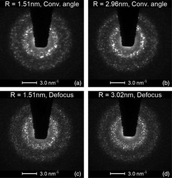
NBDPs are shown in Figure 2, they stem from measurements with constant j tot. Fundamental differences exist between NBDPs from probes created by semi-convergence angle variation, seen in Figures 2a and 2b, and defocussed ones displayed in Figures 2c and 2d. The latter consistently feature more and finer speckles at all scattering vectors k. This can be caused by phase gradients in the defocussed probes and different coherence (Gibson & Treacy, Reference Gibson and Treacy2009). Another observation is that the amount of speckles slightly increases for larger beams. This has already been discussed in the past (Hwang & Voyles, Reference Hwang and Voyles2011) and is only mentioned here for completeness. The reason for more speckles at larger R lies in an increased illuminated sample volume which results in an increased number of scattering events, leading to more speckles. As the NBDPs greatly differ between the two methods, it is reasonable to assume that the normalized variance curves themselves will differ as well. These are discussed below.

Fig. 2. Typical NBDPs of amorphous silicon from four different measurements. The exposure time of each amounts to τ = 3.2 s. The NBDPs of the experiments with standard probes in (a) and (b) exhibit less and coarser speckle compared to the ones from defocussed probes shown in (c) and (d). Furthermore, one can see that the amount of speckle slightly increases with larger probe sizes R.
Next, we analyze the normalized variance curves with respect to how the probes were formed. For this purpose, we evaluate how V(k, R) changes at the scattering vector k = 3.19 nm−1 upon increasing the probe size R. This k value marks the first peak of amorphous silicon and can be linked to reflections from {111} lattice planes. In Figure 3, the V(k = 3.19 nm−1, R) behavior of the experiment with a constant total electron dose j tot is shown. Two opposing trends can be determined from the graph. For probes created by variation of the semi-convergence angle α, the graphs feature a maximized normalized variance between R ≈ 2.00 nm and R ≈ 2.50 nm at both sample positions. This suggests that the MRO in the material is near this length scale. On the contrary, the peak normalized variance is steadily decreasing for the measurements with defocussed beams. The influence of defocus appears to overshadow subtle structural information extracted from VR-FEM and the trend in the data seems to be correlated to the amount of defocus. One further conclusion from this figure is that defocus persistently yields a reduced variance magnitude. We can exclude beam-sample interactions as being responsible for the observed differences between the two methods. There is no reason to assume that these interactions vary between the measurements as the electron energy as well as the total electron dose j tot is the same for both types of experiments. Rather, these differences likely arise due to varying illumination coherence which can be attributed to the phase gradient in the defocussed beams that suppress coherent intensity fluctuations.

Fig. 3. Normalized variance of amorphous silicon at k = 3.19 nm−1 for different probe sizes at two measurement areas. The probes were created either by semi-convergence angle variation (red data) or defocus (black data). This experiment was conducted at a constant total electron dose j tot and corresponds to measurements 1-C to 4-C and 1-D to 4-D in Table 1. The normalized variance at this scattering vector is continuously decreasing for the defocus experiment. However, V(k, R) shows a maximum at the intermediate probe sizes between R = 2.03 nm and R = 2.51 nm for the semi-convergence angle variation probes. Moreover, the latter continuously feature a larger V(k, R).
The above-mentioned results were all obtained from experiments at constant total electron dose j tot. Next, those results are compared to ones obtained from measurements with an identical areal electron density j area. In these measurements, the exposure times were adjusted to feature a comparable j area for every probe size R using the largest beam as a reference point. Consult Table 1 for exact values. Unfortunately, these experiments on amorphous silicon have a poor signal-to-noise ratio (SNR). Nonetheless, some minor conclusions can be drawn from the data which are shown in Figure 4. In this case, V(k = 3.19 nm−1, R) is constantly decreasing for both probe methods. The data points from the semi-convergence angle variation seem to converge toward a plateau at R = 1.51 nm, while the defocus ones do not do this. The plateau can be linked to the previously described behavior of V(k, R). When the experiment was performed at constant j tot, the peak normalized variance increased when changing the beam from R = 1.51 nm to R = 2.03 nm due to the influence of MRO. This contribution is still present in the experiment with identical j area but is being compensated by the decreasing SNR when decreasing the exposure time from R = 1.51 nm to R = 2.03 nm. Thus, both aspects, the increase due to MRO and decrease due to less signal, roughly cancel each other out and lead to little change for the red data points from R = 1.51 nm to R = 2.03 nm in Figure 4. The defocus experiment still yields an overall decreased normalized variance compared to the first method due to the effect of phase gradients. This is in agreement with the prediction given in the literature for a Gaussian beam (Gibson & Treacy, Reference Gibson and Treacy2009). Now, we quantify the probe characteristics of differently formed beams. Images of selected experimental probes and corresponding intensity profiles including the resulting fits can be seen in Figure 5. Generally, the fit is able to reproduce the data, even for the strongly defocussed beam. The fits onto the beams and the deduced parameters indicate that the source size σ is increasing for an increasing probe size R when it is realized by variation of the semi-convergence angle α. The results are listed in Table 2. The parameter σ amounts to approximately  $15\percnt$ of the corresponding probe size R. Since the probe size is controlled by the semi-convergence angle α, it follows that the determined σ is affected by α. A dependence of σ on the semi-convergence angle has been previously reported (Yi & Voyles, Reference Yi and Voyles2011). The source sizes σ for probes created by defocus are listed in Table 3.

Fig. 4. Normalized variance of amorphous silicon at k = 3.19 nm−1 for different probe sizes at two measurement areas. The probes were again created either by semi-convergence angle variation (red data) or defocus (black data). This experiment was conducted at a comparable areal electron density j area (measurements 4-C to 7-C and 4-D to 7-D in Table 1) where the largest beam served as a reference point. This means that the exposure time of NBDPs taken with the smaller probes were adjusted such that they had the same j area as the large probe at its respective exposure time of τ = 3.2 s. However, this results in a bad SNR such that noise dominates the result. Nonetheless, the red data points still have a larger V(k = 3.19 nm−1, R) than the black ones, identical as in Figure 3.

Fig. 5. Selected experimental STEM probes which were used for the FEM measurements. In (a) and (b), the probes were created by convergence angle variation while in (c) and (d), the desired probe size R is realized by defocus. Next to each probe its measured and fitted logarithmic intensity profiles are displayed.
Table 2. Evaluation of the Source Size σ for Probes Realized by Variation of α.

We assume an uncertainty of 10% for σ based on the stability of the fits.
Table 3. Evaluation of the Source Size σ for Probes Realized by Defocus.

Again we assume an uncertainty of  $10\percnt$ for σ based on the stability of the fits. The coherent volume fraction was calculated following Gibson & Treacy (Reference Gibson and Treacy2009).
In this case, the source size remains at a comparable level between the probes. It is close to the source size σ = 0.168 nm of the initial probe with R = 1.00 nm that was used to create the defocussed beams. This agrees with the idea that σ is seemingly reciprocally related to α as the semi-convergence angle was not changed, and thus, one can expect the source size to remain constant between the defocussed probes. We have also calculated the generalized defocus Δ = λΔf/4πρ 2 (Gibson & Treacy, Reference Gibson and Treacy2009), where  $\rho = R/\lsqb 2\sqrt {2{\rm ln}\lpar 2\rpar }\rsqb$ is the standard deviation of the undefocussed beam. By calculating this expression, the beam's coherent volume fraction can be obtained which is given by C(Δ) = 1 − exp( − π/8Δ). As the defocus increases, it creates phase gradients in the probe wave function and by this reduces the coherent fraction to, i.e., $92.09\percnt$ for the largest defocussed beam. This decrease in coherence affects the FEM results and could explain the decreased normalized variance compared to measurements from standard probes as seen in Figure 3. For FEM, we are interested in coherent diffraction such that the beam should be as coherent as possible. This implies an aberration-free beam along with a minimal σ such that the source is an ideal point source. In this case, the Airy ringing will be most pronounced and the intensity should decrease to zero at the minima. Not all microscopes might feature the necessary equipment to be able to create a large range of coherent probe sizes and defocus might be unavoidable. In such cases, we think that the referenced concept of the coherent volume fraction C(Δ) can be used as a guideline to judge whether defocus is acceptable or not. Our current results indicate that $C\lpar \Delta \rpar = 97.31\percnt$ is already unacceptably small based on the observation that at this value, V(k, R) already differs at the first peak between the two probe formation types as displayed in Figure 3. A defocussed probe can be considered acceptable for FEM if the coherent volume fraction is as close to 1 as possible, we suggest $C\lpar \Delta \rpar \gt 99.95\percnt$. The critical parameter which determines the coherent volume fraction is, beside the defocus itself, the initial probe size due to the quadratic dependence in the exponential. Applying a defocus of, e.g., 150 nm to a probe with R = 0.5 nm is much worse than applying the same amount of defocus to a probe with R = 2.0 nm.
Our observations regarding σ as well as previous ones by Yi et al. (Reference Yi, Tiemeijer and Voyles2010) can be explained by the subsequent magnification of an initial source σ 0 as shown in Figure 6. The electrons emitted from this source pass the gun lens as well as three condenser lenses termed C1, C2, and C3. At the C2 lens, there is additionally the probe forming aperture with a radius a. For simplicity, we assume no further apertures in the beam path. Each of the four lenses has a magnification M i = v i/u i where v i and u i are the image and object distance of a respective lens. Moreover, the condition L i = v i + u i+1 holds. Based on this setup, it follows that σ 4 = M 1M 2M 3M 4σ 0 = (v 1/u 1)(v 2/u 2)(v 3/u 3)(v 4/u 4)σ 0. The aperture introduces a convolution of the source function with an extent of σ 2 with Bessel functions in our extended formalism. The beam size at the σ 3 plane is then mainly controlled by the aperture along with the semi-convergence angle and no longer purely by the source. From σ 0 to σ 2, the beam size coincides with the corresponding σ i. This no longer applies for the planes of σ 3 and subsequent ones due to the convolution. Here, σ 3 and following rather denote what source size one would obtain when applying the fit from equation (2) to the beam. Further lenses, that can occur after σ 4, are omitted since they are assumed to act statically, i.e., their focal lengths do not change, implying an additional constant magnification resulting in σ Observed = M cσ 4. In the fit to the experimental electron beams, we only analyze the situation directly at the C2 lens. The fit determines σ 2 based on the observed probe which is not in the σ 3 plane. Thus, the beam undergoes a subsequent magnification such that σ Observed = M 3M 4M cσ 2 = Mσ 2. The importance of the magnification can be easily shown with equation (2). The transformation  $\tilde {x}_3 = M x_3$, $\tilde {y}_3 = M y_3$ yields for the Gaussian source term $\psi \lpar \tilde {x}_3\comma\; \tilde {y}_3\rpar \sim \exp \lpar -0.5\lpar \tilde {x}_3^{2} + \tilde {y}_3^{2}\rpar /\lpar M\sigma _2\rpar ^{2}\rpar$. Since we do not know the magnification M, we cannot determine σ 2 but only the product σ = Mσ 2. A problem lies in the fact that changes of the imaging conditions can affect M as well as σ 2. Changes in M can be estimated with the help of Figure 6 based on simple geometrical optics as described in the following.

Fig. 6. Schematic illustration on how an initial source σ 0 is imaged by four lenses along with an aperture. The blue ray path marks the path of the entire beam, while the red one shows the path of the fraction that passes the aperture. Every lens has a respective magnification M i = v i/u i resulting in different σ i at the corresponding image planes. Adjusting the illumination conditions is realized by changing the focal length of a lens. Distances and angles which are necessary for deriving expressions for the source size are displayed as well. The dashed lines after σ 4 indicate that the beam passes through further lenses but those are fixed as explained in the main text.
First, we analyze variations of the semi-convergence angle α. For this purpose, the focal lengths of the C2 and C3 lenses are adjusted which influences the angle β. We assume this angle to be proportional to the semi-convergence angle α at the sample. Knowing that v 3 = p + q, where p is a fixed distance, while q is dependent on the lens strength, and using the small-angle approximation for β, it follows that v 3 = p + a/β. At the same time, one obtains u 4 = L 3 − v 3 = L 3 − p − a/β. The combination of these equations yields
 $$\eqalign{\sigma_4\lpar \beta\rpar & = M_3 M_4 \sigma_2 \cr & = {\,p + a/\beta\over u_3}{v_4\over L_3-p-a/\beta}\sigma_2 \cr & = {v_4\over u_3}{\,p + a/\beta\over \lpar L-p\rpar -a/\beta}\sigma_2.}$$
The functional remains valid when assuming that α is proportional to β and can be used to describe the physics at the sample plane. Changing the semi-convergence angle, thus, has an seeming effect on the source size since only the magnification changes. We conclude that the actual source is independent of the semi-convergence angle. The effect of varying the radius a of the probe forming aperture on the source size can readily be seen in equation (3) as well. Again, the source σ 2 itself is unaffected, but only the magnification changes at a fixed angle β. Consequently, a smaller aperture radius yields a smaller σ 4 but an identical σ 2.
Varying the so-called spot size (for Thermo Fischer instruments the spot number) is equivalent to adjustments in the C1–C2 condenser system. This leads to changes of the source size σ 2 itself but also affects the magnification. Increasing the spot size from the setting N to N + 1 will result in v 2,N → v 2,N+1 = Wv 2,N where W < 1. We base this assumption on the fact that the spot size can only be changed in discrete steps and that each increase leads to a reduction of the maximum current by approximately  $50\percnt$ as stated in the FEI Titan-Condenser manual. With u 3,N = L 2 − v 2,N, one obtains
 $$\eqalign{\sigma_4 \lpar N\rpar & = M_1 M_2 M_3 M_4 \sigma_0 \cr & = M_1 {v_{2\comma N}\over u_2}{v_3\over u_{3\comma N}} M_4 \sigma_0 \cr & = M_1 {W^{N} v_{2\comma 1}\over u_2}{v_3\over L_2-W^{N} v_{2\comma 1}} M_4 \sigma_0 \cr & = \hat{A}{W^{N}\over \hat{B}-W^{N}} \sigma_0\comma\; }$$
with constants  $\hat {A}\comma\; \ \hat {B}$. For the third equality, the expression for v 2,N in dependence of the spot size N was inserted. The source size of interest, σ 2, changes according to σ 2 ~ W Nσ 0. Since W < 1, a larger spot size N leads to a smaller σ 2. Additionally, the magnification M 3 changes as well such that the pure dependency of σ 2 to the spot size N cannot be determined from the trend of σ 4(N) = M 3(N)M 4·σ 2(N).
Defocus is equivalent to changing the lens strength of the C3 lens. However, this does not affect σ 4 because the object plane of the subsequent lenses, like the mini-condenser lens or objective lens, remains at the same distance. Rather, only phase gradients appear which can be taken into account if the fit formalism is extended to include defocus. Then, a constant source size should be obtained which is proven by our experimental results.
Varying the beam current I by adjusting the gun lens and C1 lens influences the distances v 1 and u 2 = L 1 − v 1. In this case, the focus alterations purely affect the source size σ 2. Expressed as a function in dependence of v 1, one obtains σ 2 = Kv 1/(L 1 − v 1)·σ0 with a constant K. Hence, the smallest source is obtained for a strong excitation of the gun lens which is equivalent to small v 1 and small current. The source area πσ 2 is proportional to the beam current (Yi et al., Reference Yi, Tiemeijer and Voyles2010). In principle, this observation is related to the conservation of brightness B given by B = 4I/(πσ iδ i)2 with the current I at the plane of σ i with corresponding solid angle  $\pi \delta _i^{2}$. Apertures limit the beam current and decrease it by an amount Ω < 1. In the simplest setup, only the C2 aperture limits the current. Consequently, the current I is constant in the presented setup until the beam reaches the aperture. There, the current decreases to $I_{{\rm Ap}} = \Omega I = \Omega \cdot 1/4 \cdot B \pi \delta _i^{2} \pi \sigma _i^{2}$ for i ≥ 3. However, the exact amount of lost current does not need to be considered, but it is sufficient to restrict the analysis to the red ray path in Figure 6. This current, I Red = I Ap, is constant along the entire red ray path, its actual value depends on the gun lens setting, spot size, aperture radius, and semi-convergence angle. Adjusting the beam current by decreasing v 1 reduces the current I Red. Since we observe the red ray path, a change in v 1 has no effect on the path from the C1 lens up to the sample. This means that none of the corresponding angles change either, γi = const. for i ≥ 2. However, the ray path from σ 0 to C1 changes such that it is closer to the optical axis for smaller v 1. As the current is constant along this beam path due to the conservation of brightness, it holds that the current at the screen I Red is the same as the current at the plane of σ 2 leading to $I_{{\rm Red}} = 1/4 \cdot B \pi \gamma _2^{2} \lpar \pi \sigma _2^{2}\rpar$. As noted, γ 2 is constant for the red ray path which results in a linear relationship between the probe's screen current and its source area $\pi \sigma _2^{2}$. Also note that the red ray path is mainly controlled by the aperture's size. Its diameter should be as small as possible in order to select electrons that are closest to the optical axis and consequently are least affected by aberrations.
The dependence of the source size on the semi-convergence angle, aperture radius, and spot size is only valid if the changes are applied at a constant current. Otherwise, changing these parameters will also affect the current, leading to an additional contribution to σ 2. This contribution can be compensated by maintaining an identical probe current by means of gun lens—C1 focus variations.
One important aspect for FEM is to know what the “true” probe size R is. As FEM is a scattering technique, the relevant beam characteristic is the transverse coherence length ξ. It can be defined as the maximum length scale in the sample from which coherent interference can arise. Diffraction at length scales larger than ξ will contribute partially coherently, or even incoherently, to the intensities. Thus, it appears natural that the probe size is related to the beam's coherence, e.g., the source size σ 2. In the past, it has been demonstrated that a smaller source size equals a larger V(k, R) at identical nominal probe FWHM (Li et al., Reference Li, Bogle and Abelson2014). This goes hand in hand with the idea that σ 2 is related to the coherent scattering volume in FEM experiments. There should be a reciprocal relationship between ξ and σ 2 where ξ ~ 1/σ 2. For a perfect point source, ξ would diverge toward infinity creating a fully coherent beam, meaning that the transverse coherence length will span the entire probe. For σ 2 > 0, the transverse coherence length ξ will be finite, possibly smaller than a geometric beam size like the FWHM. Thus, one cannot simply use geometric probe sizes to define the coherent scattering volume within the sample for a finite σ 2 but should in principle use ξ. Determining ξ for a realistic multi-lens and multi-aperture TEM setup is very difficult and requires knowledge of all geometric parameters which are generally not precisely known. From an experimental point of view, researchers are advised to make their FEM probe as coherent as possible by using a TEM equipped with an FEG at a small beam current, a high spot number, and a small aperture. Assuming that one has created a probe with a transverse coherence length ξ that is larger than the probe itself, the question raises what probe size definition is suitable to extract MRO reliably? In principle, several definitions are possible such as using the FWHM, the range where the beam contains  $X\percnt$ of its current or the first zero of the Bessel function. Here, a possible solution would be to use FEM simulations with a known MRO type and size and to try to extract which probe size definitions are capable to extract the MRO size most precisely.
System II: PdNiP Metallic Glass
In Figure 7a, the normalized variance in dependence of the exposure time of the NBDPs is presented. The probe size was measured to be 0.8 nm in FWHM at a semi-convergence angle of 1.2 mrad with a beam current of 15 pA. Generally, the normalized variance curves exhibit the following trend: the longer the exposure time, the more electrons are counted in the individual pixels of the NBDPs leading to an improved SNR and the suppression of Poisson noise. It should be noted that all NBDPs were corrected for X-ray spikes on the camera, but the threshold for short exposure times is in the order of the maximum intensity of the first peak such that residual spikes can not be removed automatically. The resulting problem occurs in Figure 7a at higher k-values as single peaks which is exemplary marked with 1.

Fig. 7. Influences on the normalized variance profiles with respect to (a) the exposure time, (b) accounting for the same total dose of electrons, (c) a changed coherence by a change of beam current, and (d) a VR-FEM data set with same microscope conditions for all different probes.
The second observation is that a maximum reasonable (thickness dependent) exposure time exists such that longer exposure times do not further suppress noise, but rather increase drift effects during the NBDP acquisition. The normalized variance converges to a certain curve and the only deviation in the presented data, i.e., the first peak substructure, is due to the insufficient number of NBDPs which has been discussed elsewhere (Voyles & Muller, Reference Voyles and Muller2002; Bogle et al., Reference Bogle, Nittala, Twesten, Voyles and Abelson2010; Li et al., Reference Li, Bogle and Abelson2014). It is found that—for the current setup—exposure times greater than 4–5 s lead to minimal improvements to the noise level in the normalized variance. This is observed at k-values with insignificant structural information, for instance, at the range of 2–3.5 nm−1 as well as between the two peaks at approximately 6.5 nm−1 for Pd40Ni40P20. At these k-values, V(k, R) is in the order of 0.02 which is less than 12% with respect to the maximum of the first peak. In the literature, the noise level is excepted to range up to 40% (with respect to the first peak) in order to be identified as good SNR (e.g., Li et al., Reference Li, Bogle and Abelson2014). Furthermore, it can be stated that at least 1,000–1,500 electrons in the first ring of an NBDP are necessary (Voyles & Muller, Reference Voyles and Muller2002; Li et al., Reference Li, Bogle and Abelson2014; Radić et al., Reference Radić, Hilke, Peterlechner, Posselt and Bracht2019). Even for large k-values, the SNR is less than 20% for sufficiently long exposure times. Thus, it is reasonable to search for the right balance of a chosen exposure time with respect to thickness and drift. At t/λ ~ 0.6, this is on the order of 4–5 s at the given beam settings for Pd40Ni40P20.
Figure 7b displays VR-FEM data obtained at an identical areal electron density j area. In contrast to the j area measurement on amorphous silicon, here the smallest probe has been used as the reference probe to set up the desired experimental conditions. Using the 15 pA beam current, the dose rate is about 9.36 × 10⁷ e −/s. The dose rate normalized to the probe size of R = 0.8 nm is 9.36 × 10⁷ e −/s · 4/πR 2 ≈ 1.86 × 10⁸ e −/s nm2. This results in ≈ 3.72 × 10⁸ e −/nm2 electrons that pass through a unit area during an exposure time of 2 s. In order to have the same amount of electrons per unit area for other probe sizes, the exposure time needs to be adjusted since a change of beam current (and thus the dose rate) would change the coherence which is discussed later using Figure 7c. Using a reference probe size R ref and exposure time τ ref (here R ref = 0.8 nm and τ ref = 2 s at a semi-convergence angle of α ref = 1.2 mrad), one can calculate the new exposure time τ new at the new probe size R new via
 $$\tau_{{\rm new}} = \left({R_{{\rm new}}\over R_{{\rm ref}}}\right)^{2} \times \tau_{{\rm ref}}.$$
This results in exposure times of 5.28 and 10.12 s for the probe sizes of 1.3 and 1.8 nm as displayed in Figure 7b. It should be noted that the probe size change was obtained by adjusting the semi-convergence angle. Additionally, minor readjustments of the beam current back to the reference value of 15 pA were necessary for this procedure. It is clearly visible that keeping j area equal within the investigated volume only changes the SNR, observable via the unequal V(k, R) at high and low k-values. Thus, it can be concluded that the total dose per area within a certain measurement time has only an effect on the SNR.
The effect of an altered coherence by changing the beam current (comp. Yi et al., Reference Yi, Tiemeijer and Voyles2010) is shown in Figure 7c. As stated in Yi et al. (Reference Yi, Tiemeijer and Voyles2010), “The source area is proportional to the probe current, so only low-current probes can have the best coherence.” A smaller beam current increases the coherence and finally leads to an increase in the normalized variance as indicated by the arrow. Additionally, less current leads to decreased scattering intensity in the NBDPs such that the above stated exposure times of 4–5 s do not lead to a minimized SNR. For low-dose probes, the coherence is better but the exposure time needs to be increased to regain a sufficient SNR (Voyles & Muller, Reference Voyles and Muller2002).
In Figure 7d, the probe current was adjusted for each semi-convergence angle, resulting in reasonable accessible probe sizes with the 10 μm C2 aperture ranging from 0.8 to 8.5 nm using always identical thicknesses and exposure times. As a result, the normalized variance curves basically have the same value for high and low k-values marked with 2 and 3 in Figure 7d. Furthermore, the normalized variance curves lose features the larger the probe size or, in other words, the more the NBDP become similar to a selected area diffraction pattern such that the probe size is not anymore in the range of possible MRO. In conclusion, the changed setup for different probe sizes yields valuable results.
Comprehensive MRO studies on the PdNiP system using the current setup were recently reported in Hilke et al. (Reference Hilke, Rösner and Wilde2020) and Davani et al. (Reference Davani, Hilke, Rösner, Geissler, Gebert and Wilde2020a, Reference Davani, Hilke, Rösner, Geissler, Gebert and Wilde2020b).
Generally, microscopists should try to realize, identify, and avoid possible errors by carefully setting up the experiment and analyzing the region of interest on a sample, by EELS, EDX, HAADF-STEM, etc., beforehand in order to avoid post-acquisition corrections as described in Li et al. (Reference Li, Bogle and Abelson2014).
Summary
In this work, we examined different experimental aspects of FEM on two different disordered materials. The experiments on amorphous silicon show that the peak normalized variance from measurements with defocussed probes is continuously smaller than V(k, R) obtained from experiments with probes created by semi-convergence angle variation. Furthermore, the two experiments show different trends for the peak normalized variance in dependence of the probe size. Both observations are related to the decreasing coherence of the data acquired with defocussed beams. Consequently, defocus has to be avoided for FEM experiments.
The comparison of FEM data acquired with a constant total electron dose j tot to data with a constant areal electron density j area reveals very different trends for the peak normalized variance of a-Si. This difference can mainly be attributed to different exposure times, leading to a low SNR at small exposure times of the j area experiment with the silicon sample. Therefore, it is more important to ensure a high SNR in FEM rather than paying attention to the number of electrons that could interact with the material during acquisition. In principle, one could use the smallest probe as a reference for FEM experiments with identical j area and consequently increase the exposure time of larger beams. This has been done for Pd40Ni40P20 in the present work and normalized variance curves with a high SNR were obtained. They display the same trend as the experiment with identical j jot on this system. Because of the relatively large exposure times in this case, the method faces drift during acquisition as a main drawback. Another negative aspect of large exposure times is potential saturation or damage of the camera.
Fits of the intensity profile of the electron beams are capable to reproduce the experimental probes very well. The addition of defocus allows to fit a wider range of experimental probes and enables analysis of their source size. The results indicate that the source size is seemingly reciprocally related to the semi-convergence angle and independent of defocus. But these observations are partly illusionary, as we can only determine the product of the illumination system's magnification and the source size. The issue lies in the fact that the particular magnification is unknown. By using simple geometrical optics on a multi-lens system, we have analyzed theoretically what effect different TEM illumination settings have on the source size. Some parameters such as changing the semi-convergence angle only affect the magnification. Since we can only determine the product of magnification and source, this has a seeming effect on the source size itself. In fact, we showed that the source size remains identical for a given semi-convergence angle at constant current.
The experiments on the Pd40Ni40P20 metallic glass show that the normalized variance data converges toward nearly identical curves with increasing exposure time. However, some minor differences remain at the peaks, while the curves overlap at non-peak scattering vectors. We draw the conclusion that there exists an optimal exposure time τ 0 that gives a balance of high SNR along with sufficiently small drift during the acquisition time. This time depends on the exact experimental parameters. The existence of an optimal exposure time τ 0 leaves the question whether FEM data should be acquired at identical j tot or j area for different probe sizes obsolete; it is only necessary to find the optimal exposure time for every setup. This is achieved when the normalized variance peaks are maximized and when the normalized variance background converges as shown in Figure 7a.
The V(k, R) curves are greatly affected when varying the beam current at identical probe size: A smaller beam current yields a drastically larger peak normalized variance for the metallic glass. This is due to the linear relationship between current and σ and highlights the importance of having a small source size for coherent FEM experiments.
Our advice to obtain a small source size and by this a highly coherent beam is to use a very small beam current, a high spot number, and the smallest probe forming aperture on a TEM equipped with a FEG. Additionally, the beam current should be identical for all probes in VR-FEM experiments.
Acknowledgments
The authors acknowledge funding of our TEM equipment from the Deutsche Forschungsgemeinschaft (DFG) via the Major Research Instrumentation Programme under INST 211/719-1 FUGG. S. Hilke and M. Peterlechner gratefuly acknowledge financial support by DFG via PE 2290/2-1, D. Radić and H. Bracht by DFG via BR 1520/21-1 and M. Posselt by DFG via PO 436/9-1. Furthermore, the authors acknowledge A. Hassanpour for the sample preparation of the Pd40Ni40P20.


 Open access