


Introduction
The history of science is punctuated by the development of tools, approaches, and protocols to more richly probe the natural world (Daston & Elizabeth, Reference Daston and Elizabeth2011). Watershed discoveries have been directly linked to humanity's sophistication in designing and executing increasingly revealing experiments. The rise of clean energy (Zhang et al., Reference Zhang, Firestein, Fernando, Siriwardena, Treifeldt and Golberg2019), the silicon revolution (Van Benthem & Pennycook, Reference Van Benthem and Pennycook2007), and designer medicine (Frank, Reference Frank2017; Shen, Reference Shen2018) are just a few results of seeing the world through better spatial, chemical, and temporal lenses. Traditionally, manual approaches have kept pace with experimentation, but today all scientific domains produce data at a scale and complexity far exceeding human cognition (Baraniuk, Reference Baraniuk2011; Gupta et al., Reference Gupta, Kar, Baabdullah and Al-Khowaiter2018). This situation has yielded an ironic surplus of data and shortfall of immediately actionable knowledge, motivating the development of automation and artificial intelligence (AI) to transform experimentation (King et al., Reference King, Whelan, Jones, Reiser, Bryant, Muggleton, Kell and Oliver2004; Vasudevan et al., Reference Vasudevan, Choudhary, Mehta, Smith, Kusne, Tavazza, Vlcek, Ziatdinov, Kalinin and Hattrick-Simpers2019; Brown et al., Reference Brown, Brittman, Maccaferri, Jariwala and Celano2020; Noack et al., Reference Noack, Zwart, Ushizima, Fukuto, Yager, Elbert, Murray, Stein, Doerk, Tsai, Li, Freychet, Zhernenkov, Holman, Lee, Chen, Rotenberg, Weber, Goc, Boehm, Steffens, Mutti and Sethian2021; Stach et al., Reference Stach, DeCost, Kusne, Hattrick-Simpers, Brown, Reyes, Schrier, Billinge, Buonassisi, Foster, Gomes, Gregoire, Mehta, Montoya, Olivetti, Park, Rotenberg, Saikin, Smullin, Stanev and Maruyama2021). While some communities, such as chemical synthesis (Takeuchi et al., Reference Takeuchi, Lauterbach and Fasolka2005; Häse et al., Reference Häse, Roch and Aspuru-Guzik2019; Higgins et al., Reference Higgins, Valleti, Ziatdinov, Kalinin and Ahmadi2020; Xu et al., Reference Xu, Liu, Li, Xu and Zhu2020; Shields et al., Reference Shields, Stevens, Li, Parasram, Damani, Alvarado, Janey, Adams and Doyle2021), crystallography (Abola et al., Reference Abola, Kuhn, Earnest and Stevens2000; Arzt et al., Reference Arzt, Beteva, Cipriani, Delageniere, Felisaz, Förstner, Gordon, Launer, Lavault, Leonard, Mairs, McCarthy, McCarthy, McSweeney, Meyer, Mitchell, Monaco, Nurizzo, Ravelli, Rey, Shepard, Spruce, Svensson and Theveneau2005; Noack et al., Reference Noack, Zwart, Ushizima, Fukuto, Yager, Elbert, Murray, Stein, Doerk, Tsai, Li, Freychet, Zhernenkov, Holman, Lee, Chen, Rotenberg, Weber, Goc, Boehm, Steffens, Mutti and Sethian2021), and biology (Carragher et al., Reference Carragher, Kisseberth, Kriegman, Milligan, Potter, Pulokas and Reilein2000; King et al., Reference King, Whelan, Jones, Reiser, Bryant, Muggleton, Kell and Oliver2004; Nogales, Reference Nogales2016; Shen, Reference Shen2018), were early adopters of this paradigm, fields such as electron microscopy of hard matter have just begun this transition because of longstanding practical barriers (Kalinin et al., Reference Kalinin, Sumpter and Archibald2015; Schorb et al., Reference Schorb, Haberbosch, Hagen, Schwab and Mastronarde2019; Ede, Reference Ede2021; Hattar & Jungjohann, Reference Hattar and Jungjohann2021). Some of these barriers, such as closed or proprietary instrumentation platforms, are the result of business drivers, while others stem from a lack of accessible, standard-based experiment frameworks (Kalidindi & De Graef, Reference Kalidindi and De Graef2015; Spurgeon et al., Reference Spurgeon, Ophus, Jones, Petford-Long, Kalinin, Olszta, Dunin-Borkowski, Salmon, Hattar, Yang, Sharma, Du, Chiaramonti, Zheng, Buck, Kovarik, Penn, Li, Zhang, Murayama and Taheri2021). As a result, the adoption of data science in microscopy has been highly fragmented, with some institutions able to develop powerful custom instrumentation and analysis platforms, while others have been unable to integrate these practices into everyday analysis workflows (Maia Chagas, Reference Maia Chagas2018). There is presently a great need to design a practical and generalizable automation platform to address common use cases.
The two essential components of any automation platform are low-level instrument control and decision-making analytics. In the case of the former, researchers are typically forced to choose between accepting the control limitations set by manufacturers (often necessary to guarantee performance specifications) or designing a bespoke instrument. The community has developed multiple innovative approaches to high-throughput screening and automation (Carragher et al., Reference Carragher, Kisseberth, Kriegman, Milligan, Potter, Pulokas and Reilein2000; Mastronarde, Reference Mastronarde2003; Schorb et al., Reference Schorb, Haberbosch, Hagen, Schwab and Mastronarde2019), most prominently in the fields of cell biology (Coudray et al., Reference Coudray, Hermann, Caujolle-Bert, Karathanou, Erne-Brand, Buessler, Daum, Plitzko, Chami, Mueller, Kihl, Urban, Engel and Rémigy2011; Yin et al., Reference Yin, Brittain, Borseth, Scott, Williams, Perkins, Own, Murfitt, Torres, Kapner, Mahalingam, Bleckert, Castelli, Reid, Lee, Graham, Takeno, Bumbarger, Farrell, Reid and da Costa2020), medical diagnostics (Gurcan et al., Reference Gurcan, Boucheron, Can, Madabhushi, Rajpoot and Yener2009; Martin-Isla et al., Reference Martin-Isla, Campello, Izquierdo, Raisi-Estabragh, Baeßler, Petersen and Lekadir2020), single-particle cryo electron microscopy (Liu et al., Reference Liu, Li, Zhang, Rames, Zhang, Yu, Peng, Celis, Xu, Zou, Yang, Chen and Ren2016; Frank, Reference Frank2017), but also in crystallography (Rauch & Véron, Reference Rauch and Véron2014), semiconductor metrology (Strauss & Williamson, Reference Strauss and Williamson2013), and particle analysis (House et al., Reference House, Chen, Jin and Yang2017; Uusimaeki et al., Reference Uusimaeki, Wagner, Lipinski and Kaegi2019). More recently, manufacturers have begun to provide increased access to low-level instrument functions (Meyer et al., Reference Meyer, Dellby, Hachtel, Lovejoy, Mittelberger and Krivanek2019; Kalinin et al., Reference Kalinin, Ziatdinov, Hinkle, Jesse, Ghosh, Kelley, Lupini, Sumpter and Vasudevan2021; PyJEM). These application programming interfaces (APIs) can potentially be integrated into existing machine learning (ML) pipelines (Ziatdinov et al., Reference Ziatdinov, Ghosh, Wong and Kalinin2021) and may enable new control frameworks, such as “measure-by-wire” auto-tuning (Tejada et al., Reference Tejada, den Dekker and Van den Broek2011) and Gaussian-process-driven experimentation (Vasudevan et al., Reference Vasudevan, Choudhary, Mehta, Smith, Kusne, Tavazza, Vlcek, Ziatdinov, Kalinin and Hattrick-Simpers2019; Stach et al., Reference Stach, DeCost, Kusne, Hattrick-Simpers, Brown, Reyes, Schrier, Billinge, Buonassisi, Foster, Gomes, Gregoire, Mehta, Montoya, Olivetti, Park, Rotenberg, Saikin, Smullin, Stanev and Maruyama2021). However, because these APIs are in their incipient development phase and require programming, hardware, and microscopy expertise, few control systems have been designed to take advantage of them. Further complicating the situation, modern instruments often incorporate components from different manufacturers (e.g., cameras, spectrometers, and scan generators), whose lack of feature and access parity complicate any “open controller” design. The ideal “open controller” should (1) serve as a central communications hub for low-level instrument commands, (2) scale to include additional hardware components, (3) connect to external sources of data archival, and (4) integrate on-the-fly feedback from analytics into the control loop. Ultimately, the goal of any such system is to handle low-level commands, allowing the researcher to focus on high-level experiment design and execution. This goal does not mean that the researcher should be ignorant of the underlying operation of the instrument; rather, it acknowledges that most experiments aim to collect physically meaningful materials and chemical descriptors (e.g., morphology, texture, and local density of states) (Curtarolo et al., Reference Curtarolo, Hart, Nardelli, Mingo, Sanvito and Levy2013), rather than raw (meta)data information (e.g., stage coordinates, probe current, and detector counts).
Alongside practical low-level instrument control, decision-making analytics is another necessary part of any automation platform. Traditional instrument operation has been based on human-in-the-loop control, in which a skilled operator manually defines experimental parameters, collects data, and evaluates outputs to decide next steps. However, this approach is poorly suited to the large data volumes and types now routinely generated (Spurgeon et al., Reference Spurgeon, Ophus, Jones, Petford-Long, Kalinin, Olszta, Dunin-Borkowski, Salmon, Hattar, Yang, Sharma, Du, Chiaramonti, Zheng, Buck, Kovarik, Penn, Li, Zhang, Murayama and Taheri2021); humans have trouble analyzing higher dimensional parameter spaces, are prone to bias and omission of steps, and often cannot respond fast enough (Taheri et al., Reference Taheri, Stach, Arslan, Crozier, Kabius, LaGrange, Minor, Takeda, Tanase, Wagner and Sharma2016). Analytics approaches must therefore be developed that can quickly define actionable metrics for closed-loop control. The field of computational imaging has devised approaches (Voyles, Reference Voyles2017) to both improve data quality (e.g., denoising and distortion correction), and extract information using methods such as component analysis and ML. Deep learning approaches, such as convolutional neural networks (CNNs), have grown in popularity in microscopy because of their ability to learn generalizable models for trends in data without specific a priori knowledge of underlying physics (Ede, Reference Ede2021; Roccapriore et al., Reference Roccapriore, Kalinin and Ziatdinov2021). These methods can effectively interrogate large volumes of data across modalities (Belianinov et al., Reference Belianinov, Vasudevan, Strelcov, Steed, Yang, Tselev, Jesse, Biegalski, Shipman, Symons, Borisevich, Archibald and Kalinin2015) and can be accelerated using embedding computing hardware to reduce processing times. Among its many applications, ML has been used to effectively quantify and track atomic-scale structural motifs (Ziatdinov et al., Reference Ziatdinov, Dyck, Maksov, Li, Sang, Xiao, Unocic, Vasudevan, Jesse and Kalinin2017; Madsen et al., Reference Madsen, Liu, Kling, Wagner, Hansen, Winther and Schiøtz2018), and has shown recent successes as part of automated microscope platforms (Kalinin et al., Reference Kalinin, Ziatdinov, Hinkle, Jesse, Ghosh, Kelley, Lupini, Sumpter and Vasudevan2021; Trentino et al., Reference Trentino, Madsen, Mittelberger, Mangler, Susi, Mustonen and Kotakoski2021). Despite these benefits, CNNs are inherently constrained, since they typically require large volumes ( $100$ to >10 k images) of tediously hand-labeled or simulated training data (Aguiar et al., Reference Aguiar, Gong and Tasdizen2020). Due to the wide variety of experiments and systems studied in the microscope, such data is often time-consuming or impossible to acquire. In addition, a training set is typically selected with a predetermined task in mind, which is difficult to change on-the-fly to incorporate new insights obtained during an experiment.
Recently, few-shot ML has been proposed as one alternative approach to learn novel visual concepts based on little to no prior information about data (Altae-Tran et al., Reference Altae-Tran, Ramsundar, Pappu and Pande2017; Finn et al., Reference Finn, Abbeel and Levine2017; Rutter et al., Reference Rutter, Lagergren and Flores2019). Few-shot is part of the broader field of sparse data analytics, which targets the challenge of learning with limited data (Yao, Reference Yao2021). In this approach, offline CNN pre-training is performed once using a typical network, such as Resnet101 (He et al., Reference He, Zhang, Ren and Sun2016), followed by the online application of a meta-learner specialized using a limited number of user-provided examples; this approach has the benefit of computational efficiency (since the offline training is performed only once) and flexibility to adapt to different tasks. Few-shot has seen minimal usage within the materials science community, primarily in the analysis of electron backscatter diffraction (EBSD) patterns (Kaufmann et al., Reference Kaufmann, Lane, Liu and Vecchio2021), but it has great potential to inform triaging and classification tasks in novel scenarios. We have recently demonstrated the efficacy and flexibility of the few-shot approach for segmentation of electron microscope images (Akers et al., Reference Akers, Kautz, Trevino-Gavito, Olszta, Matthews, Wang, Du and Spurgeon2021); using just 2–10 user-provided examples in an intuitive graphical user interface (GUI) (Doty et al., Reference Doty, Gallagher, Cui, Chen, Bhushan, Oostrom, Akers and Spurgeon2021), it is possible to quickly classify microstructural features in both atomic-resolution and lower-magnification images. The output of the few-shot approach is essentially a feature map and statistics on their relative abundance. In addition, it is possible to easily extract pixel coordinates for desired features, which offers a pathway to feedback in a closed-loop automation system.
Here, we describe the design of a scanning transmission electron microscope (STEM) automation platform based on few-shot ML feature classification. We demonstrate the ability to acquire data automatically according to a predefined search pattern through a central instrument controller. This data is passed to an asynchronous communication relay, where it is processed by a separate few-shot application based on user input. The processed data is used to identify desired features, which may eventually guide the subsequent steps of an experiment. Additionally, we demonstrate that, in combination with a stage montaging algorithm, automated data collection can be performed over large regions of interest (ROIs). A particular advantage of the few-shot approach is that it can classify features and guide the system by task, which can be changed on-the-fly as new knowledge is gained. We argue that this approach may lead to more intelligent and statistical experimentation in both open- and closed-loop acquisition scenarios.
Materials and Methods
Sample Preparation
The TEM sample of molybdenum trioxide (MoO $_3$) flakes selected for this study has traditionally been utilized to calibrate diffraction rotation (Nakahara & Cullis, Reference Nakahara and Cullis1992). Small, electron transparent platelets of varying dimension (100 s nm to $\mu$m) are drop cast onto a carbon film TEM grid.
Hardware
The microscope used in this study is a probe-corrected JEOL GrandARM-300F STEM equipped with the PyJEM Python API. The data shown are acquired in STEM mode at 300 kV accelerating voltage. A convergence semi-angle of 27.5 mrad and a collection angle range of 75–515 mrad were used, yielding a close to high-angle annular dark-field (HAADF) imaging condition. Data processing is performed on a separate remote Dell Precision T5820 Workstation equipped with a Intel Xeon W-2102 2.9 GHz processor and 1GB NVIDIA Quadro NVS 310 GPU.
Automation Software
The automation system is composed of hardware and software components, each running in its own environment, and tied together by a central application. HubEM acts as the main end-use application for the system. It serves as a point for entering configuration, storing data, and directing the cooperation of other components through inter-process communication. It is implemented in C#/Python and uses Python.NET 2.5.0, a library that allows Python scripts to be called from within a .NET application.
PyJEM Wrapper is an application that wraps the PyJEM 1.0.2 Python library, allowing communication to the TEMCenter control application from JEOL. It is written in Python and runs on the JEOL PC used to control the instrument. The application receives messages from HubEM directing it to perform various functions such as stage motion and image acquisition. Image data is returned to HubEM for visualization and processing.
Stitching is performed by proprietary image stitching software running under HubEM as a library. As HubEM receives images from PyJEM Wrapper, this software is used to create an image montage for user visualization.
WizEM is the machine learning analysis engine of the system. It receives images from HubEM and processes them, returning both processed images and analysis data. It runs on a linux server and is implemented in Python 3.8., as described in the section “Few-Shot Machine Learning.”
All components (except stitching) are tied together using inter-process messaging. The custom protocol is on ZeroMQ and implemented in PyZMQ 19.0.2. It allows commands, images, and metadata to be passed from process to process. Depending on requirements, the system may use an asynchronous (Pub/Sub) or synchronous model (Request/Reply).
The distributed architecture of the system allows for interfacing new components into the system via future APIs. For instance, GMS Python allows communication to the Gatan Microscopy Suite (GMS) 3.4.3 for potential electron energy-loss spectroscopy (EELS) acquisition. It runs as a Python script in the GMS embedded scripting engine. A proof of concept has been developed in consultation with Gatan, using ZeroMQ to allow communication.
Few-Shot Machine Learning
The application for few-shot ML analysis has been described elsewhere (Doty et al., Reference Doty, Gallagher, Cui, Chen, Bhushan, Oostrom, Akers and Spurgeon2021). In brief, the application integrates Python, D3, JavaScript, HTML/CSS, and Vega-lite with Flask, a Python web framework. The front-end interactive visualization was created with JavaScript and HTML/CSS. The Flask Framework allows the inputs from the front-end user interaction to be passed as input to the Python scripts on the back-end. The Python scripts include the few-shot code (Akers et al., Reference Akers, Kautz, Trevino-Gavito, Olszta, Matthews, Wang, Du and Spurgeon2021) for processing the image and the WizEM code for receiving the image and sending back the processed image. Model execution time to perform inference on the full montage in Figure 4 is <10 s with GPU acceleration and 139 s with a desktop-level CPU only. Performance for the two tasks shown is comparable.
Image Stitching
Stitching is performed using a custom Python 3.7.1 script. It can be run locally as a library or run as a standalone application on a remote machine to gain more processing power. The script works as follows. First, the acquired images were converted to grayscale to remove redundant information, as all the RGB channels are identical. Then, the images were normalized to have mean pixel intensity of 0 and the maximum of the absolute value of intensity was normalized to 1 to adjust for differences in illumination or contrast. The cross-correlation of the two images was then computed for every possible overlap between them. While it is not computed this way for efficiency purposes, intuitively the cross-correlation can be thought of as sliding one image over the other and pointwise multiplying the pixel values of the overlapping points and then summing. Larger values of the cross-correlation correspond to better agreement in the features of the two images because similar values, either positive or negative, will square to positive contributions. If the values are dissimilar (i.e., a mixture of positive and negative values), then they tend to cancel out which leads to smaller values that indicate worse agreement. As such, this computed value is used to search the possible overlaps to find a local maximum. However, there is subtlety in how this maximum is determined, because if the image shows periodic structure, then there could be many local minima in the cross-correlation. In general, the global maximum will typically occur when the images are almost completely overlaid because there are numerous pixels that are summed, even if the overall alignment of features is poor. To compensate for this effect, and to emphasize the fact that we are prioritizing alignment of images, the cross-correlation is normalized by the number of pixels that were summed to compute the value.
Results and Discussion
The design of any external microscope control system is naturally complex, since hardware components from multiple vendors must be networked to a custom controller and analysis applications. For simplicity, we divide our design into three systems: Operation, Control, and Data Processing. The Operation System is a communication network that connects complex, low-level hardware commands to a simple, high-level user interface. The Control System potentially encompasses both open- and closed-loop data acquisition modes, based on few-shot ML feature classification. Where the Operation System abstracts hardware commands, the Control System abstracts raw data into physically meaningful control set points. We explore the operation of such a control scheme in the context of a statistical analysis of MoO $_3$ nanoparticles. Finally, the Data Processing System includes on-the-fly and post hoc registration, alignment, and stitching of imaging data. Together, this architecture may enable flexible, customizable, and automated operation of a wide range of microscopy experiments.
Operation System
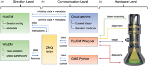
As shown in Figure 1, the backbone of this platform is a distributed Operation System for acquiring image data in an open-loop fashion, analyzing that data via few-shot ML, and then optionally automatically deciding on the next steps of an experiment in a closed-loop fashion. The distributed nature of the system allows for analysis execution on a separate dedicated ML station, which is optimized for parallel processing, acquisition and control of various instruments in a remote lab, as well as remote visualization of the process from the office or home. This remote visualization stands in contrast to remote operating schemes, which can suffer from latency and communication drop outs that impact reliability.
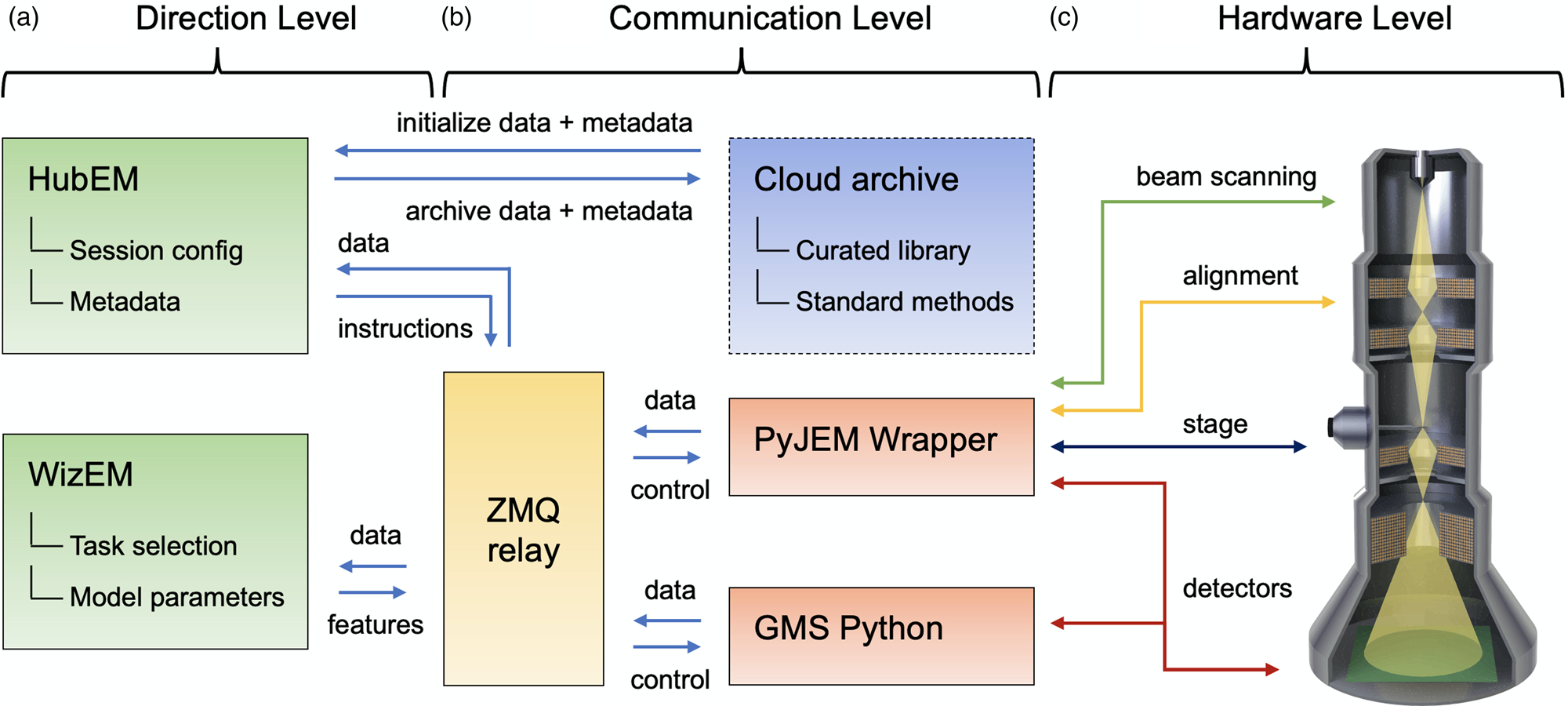
Fig. 1. Illustration of the operation system architecture, consisting of (a–c) Direction, Communication, and Hardware Levels, respectively. Arrows indicate the flow of signals between different hardware and software components at different levels of the architecture.
The operation system consists of three levels: a Direction Level, a Communication Level, and a Hardware Level. The Direction Level (Fig. 1a) includes two applications, HubEM and WizEM, designed for overall operation and few-shot ML analysis, respectively. These applications are the primary means for the end-user to interact with the microscope once a sample has been loaded and initial alignments have been performed. Each of these components is a separate process and may run on separate machines. HubEM is the main data acquisition application. It sends session configuration information to instrument controllers, receives data/metadata from them, and collates this information for a given experiment. HubEM passes instrument data to WizEM for few-shot ML analysis and receives analyzed data back for storage and real-time visualization. WizEM is a few-shot ML application featuring a browser-based Python Flask GUI (Doty et al., Reference Doty, Gallagher, Cui, Chen, Bhushan, Oostrom, Akers and Spurgeon2021). It is used to classify and record the quantity and coordinates of user-defined features in images. The results of the analysis can be displayed to the user at the end of an open-loop acquisition or eventually used as the basis for closed-loop decision making, as described in the section “Control System.”
Next, we consider the Communication Level shown Figure 1b, which connects the end-user applications to low-level hardware commands. This level is intentionally designed to minimize the amount of direct user interaction with multiple hardware sub-systems, a process that can be slow and error-prone in more traditional microscope systems. Communications between various parts of the system are handled by a central messaging relay implemented in ZeroMQ (ZMQ), a socket-based messaging protocol that has been ported to many software languages and hardware platforms (Authors, Reference Authors2021). The ZMQ publisher/subscriber model was chosen because it allows for asynchronous communication; that is, a component can publish a message and then continue with its work. For instance, HubEM can publish an image on a port subscribed to by WizEM. HubEM then continues its work of directing image acquisition, storage, and visualization, while periodically checking the WizEM port to which it subscribes. Concurrently, the WizEM code “listens” for any messages from HubEM via the ZMQ relay; these messages will contain the image to be processed by the few-shot script. WizEM analyzes the inbound data with the necessary parameters for few-shot analysis (as explained in the section “Control System” and Fig. 2). These parameters are selected by the user via the WizEM GUI at the start of, or at decision points during, an experiment. The output from the few-shot analysis is the processed image, the coordinates of each classified feature, and summary statistics for display in HubEM. The WizEM code sends the analysis output back to the ZMQ relay, where it can be received by HubEM when resources are available. The HubEM application can be connected to Pacific Northwest National Laboratory's (PNNL) institutional data repository, known as DataHub (Laboratory, Reference Laboratory2021). Data and methods, such as few-shot support sets, autoencoder selection, and model weights, can be initialized prior to an experiment and then uploaded at its conclusion.
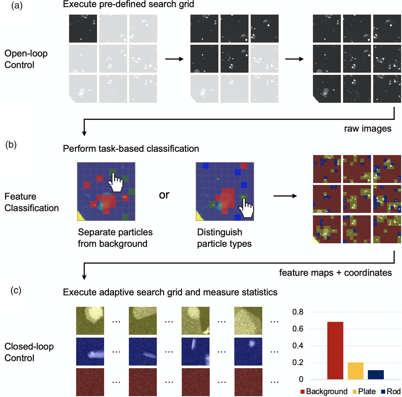
Fig. 2. Illustration of the control system architecture. (a) Open-loop Control generates search grid data that is passed through. (b) Few-shot ML Feature Classification, informing optional. (c) Closed-loop Control for complete automation. Individual image frames are taken at 20 kx magnification.
The final, and lowest-level, component of the operation system is the Hardware Level, shown in Figure 1c. This level has typically been the most challenging to implement, since direct low-level hardware controls are often unavailable or encoded in proprietary manufacturer formats. While many manufacturers have offered their own scripting languages (Mitchell & Schaffer, Reference Mitchell and Schaffer2005), these are usually inaccessible outside of siloed and limited application environments, which are incompatible with open Python or C++/C#-based programming languages. However, the recent release of APIs such as PyJEM (PyJEM) and Gatan Microscopy Suite (GMS) Python (Gatan, 2021) has finally unlocked the ability to directly interface with most critical instrument operations, including beam control, alignment, stage positioning, and detectors. We have developed a wrapper for each of these APIs to define higher level controls that are then passed through the ZMQ relay. The Hardware Level is designed to be modular and can be extended through additional wrappers as new hardware is made accessible or additional components are installed. Together, the three levels of the Operation System provide distributed control of the microscope, linking it to rich automation and analysis applications via an asynchronous communications relay.
Control System
With the operation system in place, we can now implement various instrument control modes for specific experiments. As shown in Figure 2, the instrument can be run under Open-loop Control or Closed-loop Control, separated by a process of Feature Classification. In Open-loop Control, the system executes a predefined search grid based on parameters provided by the user in the HubEM or downloaded from the DataHub institutional archive. The former approach may be used in everyday scenarios, when a user is unsure of the microstructural features contained within a sample, while the latter may be used in established large-scale screening campaigns of the same sample types or desired features. An advantage of this approach is that sampling methods can easily be standardized and shared among different instrument users or even among different laboratories.
As data are acquired via Open-loop Control, it is passed to the WizEM application for feature classification shown in Figure 2b. The support set and model parameters for an analysis can dynamically adjusted in an interactive GUI, as described in Doty et al. (Reference Doty, Gallagher, Cui, Chen, Bhushan, Oostrom, Akers and Spurgeon2021), or be initialized from the cloud. In the typical application of the former process, the user selects one of the first few acquired frames containing microstructural features of interest. An adjustable grid is dynamically super-imposed on the image, and the image is separated at these grid lines into squares, called “chips,” of which a small fraction are subsequently assigned by the user into classes to define few-shot support sets. Using just 2–10 chips for each support set, the few-shot application runs a classification analysis on the current and subsequent images sent by HubEM. Each chip in each image is classified into one of the classes indicated in the support sets. The WizEM code incorporated into the Flask application sends the colorized segmented images, class coordinates, and summary statistics back to HubEM for real-time display to the user. Once the user has defined features of interest for the few-shot analysis, it may be possible to operate the instrument in a Closed-loop Control mode, shown in Figure 2c. In this mode, the initial search grid is executed to completion according to the user's specifications. The user then pre-selects feature types to target in a follow-up analysis (termed an “adaptive search grid”). After the initial few-shot ML analysis is performed on each frame, the type and coordinates of each feature are identified and passed back to HubEM. The system may then adaptively sample desired feature types.
To illustrate a real-world example of instrument control, we consider the common use case of nanoparticle analysis. We have selected a sample of molybdenum trioxide (MoO $_3$) flakes, since it exhibits a range of particle sizes, orientations, and morphologies. MoO $_3$ is an important organic photovoltaic (OPV) precursor (Gong et al., Reference Gong, Dong, Zhao, Yu, Hu and Tan2020), has shown promise in preventing antimicrobial growth on surfaces (Zollfrank et al., Reference Zollfrank, Gutbrod, Wechsler and Guggenbichler2012), and, when reduced to Mo, can provide corrosion resistance to austenitic stainless steels (Lyon, Reference Lyon2010). As shown in Figure 2a, the user first acquires a predefined search grid within the HubEM application. This search grid is collected with specific image overlap parameters and knowledge of the stage movements to facilitate post-acquisition stitching, as will be discussed in the section “Data Processing System.” The observed distribution and orientation of the particles includes individual platelets lying both parallel and perpendicular to the primary beam (termed as “rod” and “plate,” respectively), as well as plate clusters. Particle coordinates and type can then be measured automatically via few-shot ML analysis. To do this, the initial image frames in the open-loop acquisition are passed through the ZMQ relay for asynchronous analysis in the WizEM application. In this separate application, the user selects examples of the features of interest according to a desired task, which is an important advantage of the few-shot approach. As shown in Figure 2b, the few-shot model can, for example, be tuned to distinguish all particles from the background or to separate specific particle types (e.g., plates and rods) by selecting appropriate support sets. Importantly, this task can easily be adjusted on-the-fly or in post hoc analysis as new information is acquired. Using this information, image segmentation, colorization, and statistical analysis of feature distributions is performed on subsequent data as the Open-loop Control proceeds. This information is passed back to the HubEM application, where it is presented dynamically to the user.
In the eventual final mode of Closed-loop Control, the stage may drive to specific coordinates of identified particles, adjusting magnification or acquisition settings such as beam sampling or detector. This step is the most challenging part of the experiment, since it relies on precise recall of stage position and stability of instrument alignment. Here, we propose a method for lower (20–25 kx) magnification Closed-loop Control, which is nonetheless valuable for many statistical analyses. At higher magnification, the stage is far more susceptible to mechanical imprecision and focus drift, which requires considerably more feedback in the control scheme. To better understand these challenges, we next consider the details of the acquisition and the important step of data processing for visualization and quantification.
Data Processing System
Alongside the Operation and Control Systems already described, we have developed a Data Processing System for large-area data collection, registration, and stitching of images. This processing is important to orient the user to the global position of local microstructural features and is needed for both closed-loop control and accurate statistical analysis. Building on the MoO $_3$ example discussed in the section “Control System,” we next consider the practical steps in the data acquisition process, as shown in Figure 3. While this sample is ideal because it contains different particle morphologies and orientations, it is also challenging to analyze because of the sparsity of those particles (i.e., large fraction of empty carbon background). It is therefore necessary to perform lower magnification montaging in such a way that adjacent images are overlapped in both the $x$ and $y$ stage direction. First, the user selects a single ROI within the Cu TEM grid with no tears and a high density of particles, as shown schematically in Figure 3a, with the closed red circles representing a desired feature on a support grid denoted by the blue background. This ROI is typically selected at lower magnification to increase the overall field of view (FOV), but may also be selected at higher magnification. Alternatively, fiducial markers, such as the corners of a finder grid, may be used to define the ROI. In either case, the $x$ and $y$ coordinates at the opposite corners of the ROI are defined as the collection Start and End positions, respectively.

Fig. 3. MoO $_3$ data acquisition and processing. (a) Region of interest covered by montage and calculation of stage positions between a start and end point. (b) Calculation of stage positions and observed image overlap. (c) Incremental, row-by-row stitching of images conducted via cross-correlation to produce a final montage.
Upon selection of the desired ROI, the user is prompted to enter both the magnification and the desired percent overlap between consecutive images in the montage. Combined with the Start and End positions, the montaging algorithm calculates both the number of frames as well as the stage coordinates of each individual image to be collected. Depending on user's preference, the system can collect each image in a serpentine or a sawtooth-raster search pattern, the latter of which is commonly used in commercial acquisition systems. In the serpentine pattern, a search is conducted starting in the upper left corner and moving to the right until reaching the end of the row ( $n$th frame). The search then moves down one row and back toward the left, repeating row-by-row until the $m$th row is reached and the montage is complete. In the sawtooth-raster, the search pattern also starts in the upper left, moving to the right until the end of the row is reached, just as in the serpentine pattern. At the end of the row, the direction of movement is reversed all the way back to the starting position before moving down to the next row, akin to the movement of a typewriter. From a montaging and image processing perspective there is little practical difference between these two methods, so the reduced travel time of the serpentine method is typically preferred. However, imprecision in stage movements (e.g., mechanical lash and flyback error) can lead to deviation in the precision of these approaches, particularly at higher magnification.
As shown in Figure 3b, after selection of the ROI and start of the acquisition, the program collects the first image (Image 1), at which time the feature classification process in Figure 2b can be used to define the classification task. The acquisition is optionally paused while this step is conducted, and then a second image is acquired (Image 2); the software then utilizes the predicted overlap coordinates to perform an initial image alignment check. The montaging algorithm, described next, is then employed for further refinement of the relative displacement between the two images needed for feature alignment. We note that in Figure 3b (Predicted overlap), the same particles (white asterisks) are observed in each image, but are not overlapped with one another. When further refinement of the montaging algorithm is applied (Algorithm overlap), the particles overlap (again noted by the white asterisk). Upon completion of the  $n$ frames in Row 1, the acquisition proceeds until the $m$th row of data is collected and the End position is reached. While shown in Figure 3c as complete rows, during operation each image is stitched incrementally to previous data collected in real-time. Once all stage positions have been imaged, a Final montage is calculated, at which time the user has the ability to manually or automatically select a region of interest (e.g., the particles denoted by the white asterisk) in order for the microscope to drive to the desired position and magnification.
When montaging is based solely on image capture, especially over large areas, there are many potential complications that can affect the final stitched montage. Depending on the STEM imaging conditions selected, beam drift can push the scattered diffraction discs closer to a given detector (e.g., strong diffraction onto a dark-field detector) that can skew imaging conditions from the first to the last image collected. As already mentioned, particle sparsity or clustering within the ROI can also present difficulties. For example, if the magnification is set too high, there may be regions within adjacent areas that have no significant contrast or features for registration. Such a situation might be encountered in large area particle analysis, as well as in grain distributions of uniform contrast. Understanding the stage motion is imperative in these cases, because the predicted image position can be utilized. Lastly, imprecise stage motion and image timing are important considerations. If the stage is moving during image capture, images can become blurred. In addition, if the area of interest is too large, sample height change can affect the image quality due to large defocus.
In light of these complications, we have evaluated image stitching approaches based on knowledge of the stage motion, as well as those solely based on image features. In principle, the simplest method is the former, in which prediction based on stage motion is used to calculated the overlap between two images directly. However, this method leads to artifacts in the stitched image due to a variety of practical factors related to high-throughput stage movement and image acquisition (Yin et al., Reference Yin, Brittain, Borseth, Scott, Williams, Perkins, Own, Murfitt, Torres, Kapner, Mahalingam, Bleckert, Castelli, Reid, Lee, Graham, Takeno, Bumbarger, Farrell, Reid and da Costa2020). For example, in some instances, motor hysteresis or stage lash causes a stage position to deviate from an issued command. An example of where the “predicted overlap” fails to accurately stitch adjacent images is shown in Figure 3b. Image-by-image corrections must therefore be performed post hoc using either manual or automated approaches. Manual stitching works surprisingly well for small numbers of images because the human eye is good at detecting patterns. However, this process is very time intensive, does not scale well to large montages, and cannot be automated within a program for automatic acquisition.
To automate this process, the community has developed several standalone software packages (Schindelin et al., Reference Schindelin, Arganda-Carreras, Frise, Kaynig, Longair, Pietzsch, Preibisch, Rueden, Saalfeld, Schmid, Tinevez, White, Hartenstein, Elicieri, Tomancak and Cardona2012; Schneider et al., Reference Schneider, Rasband and Elicieri2012; Rueden et al., Reference Rueden, Schindelin, Hiner, DeZonia, Walter, Arena and Eliceiri2017), but these do not provide the user with immediate feedback while directly interfacing with the microscope. As part of the processing system, we have developed an image-based registration script to dynamically align and stitch images during an acquisition. At a high level, the algorithm functions by computing the cross-correlation of adjacent images quickly using the Convolution Theorem as implemented in SciPy's signal processing library (Virtanen et al., Reference Virtanen, Gommers, Oliphant, Haberland, Reddy, Cournapeau, Burovski, Peterson, Weckesser, Bright, van der Walt, Brett, Wilson, Millman, Mayorov, Nelson, Jones, Kern, Larson, Carey, Polat, Feng, Moore, VanderPlas, Laxalde, Perktold, Cimrman, Henriksen, Quintero, Harris, Archibald, Ribeiro, Pedregosa and van Mulbregt2020), and then identifies the peak of the cross-correlation to find the correct displacement for maximum alignment. From this normalized cross-correlation, the best alignment is determined from the local maximum closest to predicted overlap, which is shown in the right portion of Figure 3b, labeled “Algorithm Overlap.” This alignment process then repeats for every image as it is acquired to build up the overall montage. After processing the raw images, the same corrections can be applied to the few-shot classified montage, providing the user with a global survey of statistics on feature distributions in their sample. As seen in Figure 3c, there is a clear qualitative improvement to the image stitching using this method. This is particularly important when identifying the number of particles, because in the case of Figure 3b, the starred particle would be erroneously double counted. On a more quantitative level, the quality of the stitch can be measured through the sum of squared errors (SSE) in the difference between the two image pixels. To illustrate the increase in quality, the predicted overlap in Figure 3b shows an SSE value of  $1.66 \times 10^{8}$, while the stitched version using the algorithm has an SSE value of $7.86 \times 10^{7}$. However, because there is a different amount of overlap in each case, a more representative statistic is the total SSE divided by the number of overlapping pixels. With this normalization, the improvement is even more clear as the SSE per pixel in the predicted overlap case is 2900 while the SSE per pixel in the stitched case is only 612.
Provided with a successfully stitched montage, the system can automatically perform task-based classification, as shown in Figure 4. Proper stitching ensures that accurate particle morphologies and counts are passed to the few-shot code for classification. At this stage, the user will pre-select support set examples corresponding to their task. For example, they may choose to separate all particles from the background (as shown in Fig. 4a) or they may wish to distinguish different particle types, such as plates and rods (as shown in Fig. 4b). They manually select a few examples (1–3 in this case) of each feature type of interest and the few-shot code uses these as its class prototypes. The advantage of this approach is three-fold: first, tasks can easily be changed at will without extensive hand labeling; second, classification can be performed in a matter of seconds compared to minutes of hand labeling; and third, classification can be easily scaled to dozens or hundreds of frames for high-speed experimentation. As we have previously shown (Akers et al., Reference Akers, Kautz, Trevino-Gavito, Olszta, Matthews, Wang, Du and Spurgeon2021), these tasks are not limited to labeling of particles and the same pretrained model can be used for other tasks, such as classification of phases and interfaces. Using this approach, it is possible to generate both rich statistical analyses and identify coordinates of desired features for subsequent closed-loop acquisition.

Fig. 4. Automated data collection and task-based classification. (a,b) Few-shot classified stitched montage, with support set examples and statistics on each identified class, for tasks of separating all particles from background and distinguishing particle types, respectively.
Conclusion
We demonstrate the design of an automation system combining low-level instrument communication with task-based classification based on few-shot ML. This system provides a practical abstraction of low-level hardware components from multiple manufacturers, which can be easily programmed through intuitive GUI applications by the end-user. It allows for microscope operation based on task-based, high-throughput statistical analysis, in contrast to more traditional automation approaches that are more labor-intensive and inflexible.
Future developments will continue to improve and extend the functionality of the automation system. In particular, reliable stage motion is a crucial enabler for the proposed closed-loop data acquisition process; better understanding of stages and improvements in hardware will help address current shortcomings, such as atomic-resolution montaging. Automated corrections (Xu et al., Reference Xu, Kumar and LeBeau2021) for focusing and beam alignment will also become important during high-magnification acquisitions. The integration of additional imaging modalities, such as diffraction and spectroscopy, is possible and will greatly extend the utility of the system. These modalities may be either pre-selected by the user or triggered in the presence of particular features identified by the few-shot ML. The use of additional APIs and recall of results from publicly available databases (Jain et al., Reference Jain, Ong, Hautier, Chen, Richards, Dacek, Cholia, Gunter, Skinner, Ceder and Persson2013; Blaiszik et al., Reference Blaiszik, Chard, Pruyne, Ananthakrishnan, Tuecke and Foster2016, Reference Blaiszik, Ward, Schwarting, Gaff, Chard, Pike, Chard and Foster2019), will further inform ML models, improving their interpretability and performance. Future designs may also integrate richer physics-based ML models or additional processing steps to enhance feature detection and improve the system control loop. Improved models may then, in turn, be passed back to public databases for wider dissemination. In this way, both results and analysis protocols can be shared to the broader community. Together, this research presents a model for more statistical and quantifiable electron microscopy. Moving forward, increasingly automated, and eventually autonomous approaches will enable richer and more standardizable experimentation, helping to transform the process of discovery across all scientific domains.
Acknowledgments
We thank Drs. Elizabeth Kautz and Kayla Yano for reviewing the manuscript and assisting with benchmarking. We also acknowledge the help of Ms. Christina Doty in montage colorization. This research was supported by the I3T Commercialization Laboratory Directed Research and Development (LDRD) program at Pacific Northwest National Laboratory (PNNL). PNNL is a multiprogram national laboratory operated for the U.S. Department of Energy (DOE) by Battelle Memorial Institute under Contract No. DE-AC05-76RL0-1830. The few-shot ML code development was also supported by the Chemical Dynamics Initiative (CDi) LDRD program, with some initial code development performed under the Nuclear Process Science Initiative (NPSI) LDRD program. The system was constructed in the Radiological Microscopy Suite (RMS), located in the Radiochemical Processing Laboratory (RPL) at PNNL. Some sample preparation was performed at the Environmental Molecular Sciences Laboratory (EMSL), a national scientific user facility sponsored by the Department of Energy's Office of Biological and Environmental Research and located at PNNL.
Conflict of interest
The authors declare that they have no competing interest.
Data availability statement
The raw and processed MoO $_3$ frames shown are available on FigShare at https://doi.org/10.6084/m9.figshare.14850102.v2. Additional details on the scripting and hardware configuration are available from the authors upon reasonable request.


 Open access