


1 Introduction
People make many decisions between a present alternative and a potential future prospect. Decision involving tradeoffs among outcomes at different points of time is referred to as intertemporal choice (Reference Frederick, Loewenstein and O’donoghueFrederick, Loewenstein & O’donoghue, 2002; Reference Prelec and LoewensteinPrelec & Loewenstein, 1991). For example, the decision to deposit part of one’s income into a bank instead of immediately spending the money can be interpreted as an intertemporal choice. In this case, one option is to purchase some goods with the money to fulfill one’s needs instantly or to save the money and gain more in the future (Reference Dai and BusemeyerDai & Busemeyer, 2014). Substantial research reveals that intertemporal choices between a smaller-sooner (SS) reward and a larger-later one can be characterized by a hyperbolic discounting function in which the greater the delay in receiving the rewards, the more these rewards are discounted (Reference AinslieAinslie, 1975; Reference Frederick, Loewenstein and O’donoghueFrederick et al., 2002). A single hyperbolic discount rate (k value) describes intertemporal choices, such that a lower k value indicates slower discounting of future outcomes and thus more patient choices, whereas a higher k value indicates steeper delay discounting and more impatient choices.
Intertemporal choice theories face challenges of accounting for known systematic inconsistencies in human decisions (Reference Roelofsma and ReadRoelofsma & Read, 2000). An example is the time preference reversal, which involves systematic inconsistencies between preferences and bids. Reference Tversky, Slovic and KahnemanTversky, Slovic and Kahneman (1990) first demonstrated this phenomenon by presenting options of varied sums of money to be received at different times in the future. For instance, one option might offer $1,660 in 18 months (SS option), and the other may offer $3,550 in 10 years (LL option). When faced with this pair of options, respondents often choose the SS option. However, when providing prices for the same exact options, most people assign a higher price to the LL option. These two decisions seem to contradict each other. The SS option cannot be both better and worse than the LL option. This preference reversal phenomenon constitutes a violation of procedure invariance (Reference Stalmeier, Wakker and BezembinderStalmeier, Wakker & Bezembinder, 1997; Reference Tversky, Slovic and KahnemanTversky et al., 1990), because the preferences should not change on the basis of their measurements.
Despite its apparent irrationality, time preference reversal is replicated in several studies. Initially, Tversky et al. (1990) designed four groups of intertemporal options and asked participants to state direct preferences between the SS and LL options or place a value on each option in the form of “the smallest immediate cash payment for which they would be willing to exchange the delayed payment.” Participants exhibited time preference reversals, that is, the SS option was preferred, but the LL option obtained a higher present value. The mean frequency of time preference reversals in the study was 52%. Subsequently, this effect was replicated when participants were incentivized by real payments (Reference BohmBohm, 1994). However, replacing hypothetical funds with real-payment tests reduced the time preference reversal rates to 19%. Further evidence showed that the time preference reversals persisted even when the outcomes of the two intertemporal options were identical, and most participants retained their responses after being informed of their inconsistencies (Reference Stalmeier, Wakker and BezembinderStalmeier et al., 1997).
Several explanations have been suggested to account for the time preference reversals, which may be caused by a disparity between the cognitive processes used in the choice and bid (valuation) tasks (Reference LoomesLoomes, 1990). First, attention allocation may vary in the two tasks. According to the contingent weighting hypothesis (Reference Mellers, Ordoñez and BirnbaumMellers, Ordoñez & Birnbaum, 1992; Reference Tversky, Sattath and SlovicTversky, Sattath & Slovic, 1988), the attribute weights are closer to lexicographic (i.e., closer to all-or-none) in choice than bid tasks, which leads to the most important attribute being weighted even more heavily in choice (Reference SlovicSlovic, 1975; Reference Tversky, Sattath and SlovicTversky et al., 1988). Given the impatience of most people (Reference Loewenstein and PrelecLoewenstein & Prelec, 1993; Reference Weber, Johnson, Milch, Chang, Brodscholl and GoldsteinWeber et al., 2007), the delay attribute is weighted more than the outcome attribute in the choice task. By contrast, the outcome attribute is weighted more during bids due to the compatibility effect (Reference SlovicSlovic, 1975; Reference Tversky, Sattath and SlovicTversky et al., 1988), whereby attributes that are compatible with the output are given extra weight. From an evidence accumulation perspective, an attribute that receives increasing weight during the decision making also gains increasing decision weight (Reference Ashby, Yechiam and Ben-EliezerAshby, Yechiam & Ben-Eliezer, 2018; Reference Busemeyer and TownsendBusemeyer & Townsend, 1993; Reference Usher and McClellandUsher & McClelland, 2001). Thus, we can infer that the delay attribute receives more attention in the choice than bid task.
Second, cognitive effort may vary in the two tasks. According to the strategy compatibility hypothesis (Reference Stalmeier, Wakker and BezembinderStalmeier et al., 1997), choosing is basically a qualitative activity and participants are thus inclined to use a qualitative strategy in decision making. Therefore, participants tend to simply choose the option that appears best for the most important attribute (i.e., delay), thus avoiding the necessity of comparing tradeoffs for different attributes. This intuitive strategy is based on the heuristic system (Reference EvansEvans, 2003; Reference Kahneman, Frederick, Gilovich, Griffin and KahnemanKahneman & Frederick, 2002; Reference SlomanSloman, 1996) and leads to low-level cognitive effort in the choice task. In addition, this intuitive choice is likely affected by impulsivity (Reference Glimcher, Kable and LouieGlimcher, Kable & Louie, 2007; Reference Ripke, Hubner, Mennigen, Muller, Rodehacke, Schmidt, Jacob and SmolkaRipke et al., 2012). By contrast, valuation is a quantitative activity, and participants weigh a favorable tradeoff for one attribute against an unfavorable tradeoff for another. Thus, the value system is balanced. Therefore, participants tend to apply a deliberate strategy on the basis of analysis (Reference EvansEvans, 2003; Reference Kahneman, Frederick, Gilovich, Griffin and KahnemanKahneman & Frederick, 2002; Reference SlomanSloman, 1996) in the bid task, leading to high-level cognitive effort.
These two hypotheses have not been examined in time preference reversals. By using an eye-tracking technology, the present study aims to investigate the cognitive processes in time preference reversals and examine the different explanations outlined above. First, establishing the differences in attention allocation during choice and bid tasks is useful to examine the contingent weighting hypothesis. To illustrate, individual attention allocation is related to subjective valuations when evaluating consumer goods (Reference Ashby, Dickert and GlöcknerAshby, Dickert & Glöckner, 2012; Reference Ashby, Walasek and GlöcknerAshby, Walasek & Glöckner, 2015) or risky options (Reference Ashby, Yechiam and Ben-EliezerAshby et al., 2018). The relationship between attention and choice is also established in risky choice (Reference Brandstätter and KörnerBrandstätter & Körner, 2014; Reference Glöckner and HerboldGlöckner & Herbold, 2011; Reference Stewart, Hermens and MatthewsStewart, Hermens & Matthews, 2015) and intertemporal choice (Reference Franco–Watkins, Mattson and JacksonFranco–Watkins, Mattson & Jackson, 2016; Reference Sui, Liu and RaoLiu et al., 2020). Reference Kim, Seligman and KableKim, Seligman and Kable (2012) replicated the preference reversals in risky choice and found that this effect occurred with a shift in fixations of the two attributes, with people fixating more on the probability attribute during choices and more on outcome attribute during bids. Subsequent research verified this finding (Reference Alós-Ferrer, Jaudas and RitschelAlós-Ferrer, Jaudas & Ritschel, 2021).
Second, establishing the differences in cognitive effort during the two tasks is useful to examine the strategy compatibility hypothesis. The mean fixation duration, which refers to the average duration of single fixations in a decision, can reflect “the degree of digging into the information” (Reference Wang, Yang, Liu, Cao and MaWang, Yang, Liu, Cao & Ma, 2014). Long mean fixation duration may indicate high levels of cognitive effort (Reference Amblee, Ullah and KimAmblee, Ullah & Kim, 2017; Reference Horstmann, Ahlgrimm and GlöcknerHorstmann, Ahlgrimm & Glöckner, 2009; Reference Velichkovsky, Challis and VelichkovskyVelichkovsky, 1999) and can be informative for cognitive processes in decision-making research (Reference Fiedler and GlöcknerFiedler & Glöckner, 2012). The mean fixation duration is examined during risky decision making and shows that deliberate calculation of weighted sums accompanies long fixations, whereas more intuitive or superficial information processing accompanies shorter fixations (Reference Horstmann, Ahlgrimm and GlöcknerHorstmann et al., 2009; Reference Su, Rao, Sun, Du, Li and LiSu et al., 2013). In addition, the mean fixation duration between gambles increases with decreasing expected value difference (Reference Fiedler and GlöcknerFiedler & Glöckner, 2012), which can potentially lead to qualitative changes in information processing and thus use thorough, effortful, and deliberate information processing. Reference Rubaltelli, Dickert and SlovicRubaltelli, Dickert, and Slovic (2012) found that the mean fixation duration and pupil dilations were greater when participants were providing a price for a gamble rather than rating the attractiveness for it, indicating that participants were more likely to engage in a deliberative thinking strategy in the pricing task rather than the rating task.
The purposes of the present study are three-fold. First, given that decision options in previous studies are intensively designed in paper-and-pencil questionnaires (Reference BohmBohm, 1994; Reference Stalmeier, Wakker and BezembinderStalmeier et al., 1997; Reference Tversky, Slovic and KahnemanTversky et al., 1990), we aim to test the time preference reversals in a wider range of intertemporal options. Two tasks are carried out in the present study, a choice task in which participants indicate their preference between a pair of SS and LL options, and a bid task in which participants indicate their valuations of intertemporal options. We assume that individuals exhibit time preference reversals (H1). Specifically, individuals are more likely to choose the SS option in the choice task but assign higher value for the LL option in the bid task.
Second, the cognitive processes in time preference reversals are examined using an eye-tracking technology to examine different hypotheses. According to the contingent weighting hypothesis, the outcome attribute is given more weight and thus receives more attention in the bid task than the choice task. According to the strategy compatibility hypothesis, people exert more effort and deliberation and thus show longer fixations in the bid task than the choice task. We thus assume that the bid task gains more dwell time on the outcome attribute (i.e., the outcome attribute receives more attention) and longer fixations than the choice task (H2). In addition, previous studies showed that the eye-tracking measures can explain the trial-by-trial variabilities and predict subsequent choices (Reference Sui, Liu and RaoLiu et al., 2020; Reference Sui, Liu and RaoSui, Liu & Rao, 2020). Therefore, we assume that the effect of task (choice task vs. bid task) on choices/bids can be mediated by the proportion of dwell time and mean fixation duration (H3). Specifically, compared with the choice task, the bid task gains more dwell time on the outcome attribute and longer fixations, thereby leading to an increase in preference on the LL options.
Third, we also examine whether individual differences on impulsivity and maximizing tendencies are related to the time preference reversals. As mentioned earlier, individuals in the choice task tend to rapidly discount the future, which is associated with self-reported measures of impulsivity (Reference Dom, D’Haene, Hulstijn and SabbeDom, D’Haene, Hulstijn & Sabbe, 2006; Reference Kirby and PetryKirby & Petry, 2004). However, individuals may apply a deliberate strategy in the bid task, and thus the relationship between temporal discounting and impulsivity is weak. Therefore, we assume that the task moderates the link between the individual differences in impulsivity and participants’ discounting rates (H4). In addition, the relationship between individual differences in maximizing tendencies and time preference reversals is tested. People who score high on measures of maximizing tendencies are more likely to adopt the deliberate maximizing strategy (Reference SchwartzSchwartz, 2015; Reference Schwartz, Ward, Monterosso, Lyubomirsky, White and LehmanSchwartz et al., 2002), thus leading to consistencies between choices and bids. Therefore, individual maximizing tendencies can be assumed to negatively predict their time preference reversals (H5).
Here we present two studies to examine the underlying process in time preference reversal. In Study 1, we conducted two tasks (i.e., the choice and bid tasks) and monitored participants’ eye movements to test our hypotheses. We improved the experimental design and conducted a pre-registered Study 2 (see the pre-registration on Open Science Framework at https://osf.io/zh3s7/) after the first round of reviews at this journal. The main findings of Study 1 were replicated in Study 2.
2 Study 1
2.1 Method
2.1.1 Participants
G∗Power (Version 3.1.9.2) (Reference Faul, Erdfelder, Lang and BuchnerFaul, Erdfelder, Lang & Buchner, 2007) is used to calculate the required number of participants to achieve 95% power and detect a medium effect (Cohen’s d = 0.5) with a paired t-test. The required sample size was N = 54. A total of 60 college students (65% female, M age = 21.6 ± 2.1) were recruited as participants in the current study. Participants received 40 yuan (RMB; approximately US$6.1) in cash for participation and an additional amount (1.1–9.9 yuan) determined by their performance in the experiment, with an average payment of 45 yuan (approximately US$6.8). All participants had normal or corrected-to-normal vision and provided written informed consent prior to the experiment.
2.1.2 Apparatus
An EyeLink 1000 plus eye-tracker (SR Research, Ontario, Canada) monitored the eye movements of participants during the experiment. The visual display was presented on a 17-inch LCD monitor (with a refresh rate of 60 Hz) controlled by a Dell PC. The screen resolution was 1024 × 768 pixels, and the screen subtended a visual angle of 36∘ horizontally and 29∘ vertically. Participants were seated at approximately 58 cm from the screen, and a chin rest was used to minimize head movements. Participants viewed the stimuli with both eyes, but eye movement data were only collected from the right eye. Participants responded to the stimuli using a keyboard.
2.1.3 Stimuli
The stimuli consisted of 50 pairs of intertemporal options obtained through random computer generation (the stimuli are included in the supplementary materials). Each pair contained one each of the SS and LL options. All options involved gains only. The outcomes were 2-digit numbers multiplied by 10, with a range of 120–990. The delays ranged between 11–99 days. The (horizontal/vertical) center-to-center distance between any two values was greater than 5∘, which ensured the proper fixation of values and that peripheral identification of an adjacent value was impossible (Rayner, 1998, 2009).
2.1.4 Task
Participants completed two tasks in the experiment, namely, choice and bid. In the choice task, participants indicated their preference between a pair of SS and LL options. A total of 100 choice trials were presented in two blocks of the same 50 pairs of options. Participants had unlimited time to choose between the two options. In the bid task, participants were requested to indicate their exact valuation of the intertemporal option. That is, they should bid an amount that would make them indifferent between obtaining the intertemporal option or gaining the amount they bid. Participants were presented with a total of 100 bid trials in two blocks of 50 trials. Bidding time was unlimited, and participants indicated their bids by pressing corresponding keys on the keyboard.
Each pair of options was presented twice during the choice trials, with the left–right placement of options switching between presentations. The same options used in the choice task were shown once individually in the bid task. In the choice task, two intertemporal options were shown on the screen side-by-side. In the bid task, the stimulus contained one intertemporal option shown on the left side and a bid prompt shown on the right side of the screen (see Figure 1).

Figure 1: Trial procedure and timing in (a) the choice task and (b) the bid task in Study 1.
The orders of tasks and placement of attributes (i.e., delay or outcome) were counterbalanced across participants. For the order of tasks, half the participants completed the choice task first, whereas the other half completed the bid task first. For the placement of attributes, half the participants saw delay as the top number, and the other half saw outcome as the top number. The options were presented in randomized order for each participant in each decision format.
To further incentivize their cooperation, the participants were informed that at the end of the experiment, one of their trials would be randomly selected to receive a real reward in a discount rate. If a choice trial was selected, participants were paid according to their decisions on that trial and received a real delayed reward (the delay of the option was multiplied by a rate of 0.1, and the outcome of the option was multiplied by a rate of 0.01). If a bid trial was selected, participants were paid using the Becker–DeGroot–Marschak method (Reference Becker, DeGroot and MarschakBecker, DeGroot & Marschak, 1964), which is widely used as an effective incentive in bid tasks (Reference Ashby, Yechiam and Ben-EliezerAshby et al., 2018; Reference Kim, Seligman and KableKim et al., 2012; Reference LoomesLoomes, 1990). Specifically, a random number was generated between 0 and the outcome attribute of the selected option, and this number was compared with the participant’s valuation. If the number was greater than his/her valuation, the participants would receive his/her valuation (at a rate of 0.01). If the number was no more than the valuation, the participant would be paid by the selected option (the delay of the option was multiplied by a rate of 0.1, and the outcome of the option was multiplied by a rate of 0.01).
2.1.5 Procedure
Upon entering the laboratory, participants received general instructions regarding the experiment and were asked to sign the informed consent. The chair was adjusted to ensure participant comfort. A 5-point calibration and validation procedure was used. The maximum error of validation was 0.5 degrees in the visual angle. In both tasks, two practice trials were first presented to familiarize the participants with the experiment procedure.
During a choice trial, a fixation disc appeared at the center of the screen. The disc also served as a drift check for the eye tracker. When fixation was registered, the participants pressed the space key to view the options. The screen showed the word “Choice” at the center for 1,000 ms, followed by two side-by-side options. Participants had unlimited time to choose between the two options, pressing “F” to choose the option on the left or “J” to choose the option on the right. After participants submitted their responses, a feedback with a check mark on the side of the chosen option was presented for 1,000 ms. See Figure 1a.
During a bid trial, a fixation disc appeared at the center of the screen. The disc also served as a drift check for the eye tracker. When fixation was registered, the participants pressed the space key to view an intertemporal option. The screen showed the word “Bid” for 1,000 ms, followed by one option on the left. Participants had unlimited time to input their bids using a keyboard and to submit their response by pressing the “Enter” key. Submitted bids were considered final, and a feedback with the amount bid was presented for 1,000 ms. See Figure 1b.
2.1.6 Questionnaires
After completing the two tasks, the participants were asked to complete two questionnaires, namely, the Maximization Scale (MS) (Reference Schwartz, Ward, Monterosso, Lyubomirsky, White and LehmanSchwartz et al., 2002) and the Barratt Impulsive Scale (BIS) (Reference Patton, Stanford and BarrattPatton, Stanford & Barratt, 1995).
The BIS (Version 11; BIS-11; Reference Patton, Stanford and BarrattPatton et al., 1995) is a 30-item self-report measure designed to assess general impulsiveness (Reference Reise, Moore, Sabb, Brown and LondonReise, Moore, Sabb, Brown & London, 2013; Reference Stanford, Mathias, Dougherty, Lake, Anderson and PattonStanford et al., 2009). The items are scored on a 5-point scale (1 = rarely never, 5 = almost always/always). High summed scores for all items indicate high levels of impulsiveness (Reference Patton, Stanford and BarrattPatton et al., 1995). A composite BIS score shows acceptable reliability (Cronbach’s alpha = 0.86).
The MS (Reference Schwartz, Ward, Monterosso, Lyubomirsky, White and LehmanSchwartz et al., 2002) measures the maximizing tendencies with 13 statements (e.g., “No matter what I do, I have the highest standards for myself.”). Participants indicate the degree to which they agree or disagree with each statement on a 7-point scale (1 = strongly disagree, 7 = strongly agree). MS is considered as a unitary scale where high scores refer to maximizing and low scores refer to satisficing (Reference SchwartzSchwartz, 2015; Reference Schwartz, Ward, Monterosso, Lyubomirsky, White and LehmanSchwartz et al., 2002). A composite MS score shows acceptable reliability (Cronbach’s alpha = 0.74).
2.1.7 Data analysis
Preprocessing of eye-tracking data
Eye-movement data were analyzed using the EyeLink Data Viewer (SR Research, Ottawa, Ontario, Canada). Fixations were defined as periods of a relatively stable gaze between two saccades, but fixations shorter than 50 ms were excluded from the analyses. In the choice task, four non-overlapping, identically sized (10.8∘ × 7.7∘ visual angle) rectangular regions of interest (ROIs) around each piece of information (i.e., outcome and delay) were defined. In the bid task, two non-overlapping, identically sized (10.8∘ × 7.7∘ visual angle) rectangular ROIs were defined.
Eye-tracking measures
The following two eye-tracking measures are used to test H2. First, the outcome–gaze–proportion (OGP) provides an index of the proportion of time attention that is allocated to the outcome attribute of an intertemporal option (Reference Amasino, Sullivan, Kranton and HuettelAmasino, Sullivan, Kranton & Huettel, 2019; Reference Ashby, Yechiam and Ben-EliezerAshby et al., 2018; Reference Franco–Watkins, Mattson and JacksonFranco–Watkins et al., 2016).
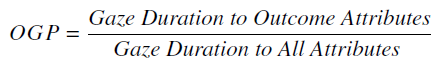
OGP values higher than 0.50 indicate that more attention is given to outcome attributes than delay attributes, and those lower than 0.50 indicate more attention toward delay attributes. OGP = 0.50 indicates equal distribution of attention between outcome and delay attributes.
Second, the mean fixation duration (MFD) is calculated by adding the duration of all fixations during a trial and dividing the total by the number of fixations. As mentioned above, MFD is sensitive to cognitive effort (Reference Amblee, Ullah and KimAmblee et al., 2017).
Estimating discount factor
The hyperbolic model is used to estimate the discount factors in both tasks. According to the hyperbolic model, the subjective value of a delayed reward is discounted according to
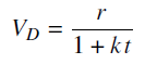
where r is the magnitude of a reward offered at delay t, and the individually determined parameter k is the discount factor (Reference Mazur, Commons, Mazur, Nevin and RachlinMazur, 1987). As the value of k increases, the person discounts the future more steeply (Reference Kirby and PetryKirby & Petry, 2004; Reference Kirby, Petry and BickelKirby, Petry & Bickel, 1999). Therefore, k can be considered as an impulsiveness parameter, with high values corresponding to high levels of impulsiveness (Reference Herrnstein, Bradshaw, Szabadi and LoweHerrnstein, 1981). The hyperbolic model is used for its good fit to behavior with a single parameter (k) summarizing preferences (Reference Rodriguez, Turner and McClureRodriguez, Turner & McClure, 2014).
For choices, we fit a logistic regression that assumes the likelihood of selecting an LL option (P LL) as
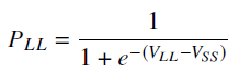
where V LL and V SS are given by Equation 2. We fitted Equation 3 for participants to their observed choices to determine the maximum likelihood estimate of k choice. Data from four participants were not convergent, and thus their k values were excluded from the discount factor analysis.
For bids, we fit a model that assumes the participant bid as equal to the discounted value of the intertemporal option. Least squares are used to estimate each participant’s k value.
Mixed effect model
We used mixed effect models with the random effects of the participant and item to analyze our data using the lme4 and lmerTest packages in the R statistical environment (Reference Bates, Maechler, Bolker and WalkerBates, Maechler, Bolker & Walker, 2015; Reference Kuznetsova, Brockhoff and ChristensenKuznetsova, Brockhoff & Christensen, 2017). Following the suggestions of Reference Barr, Levy, Scheepers and TilyBarr, Levy, Scheepers, and Tily (2013), the random effects structure was kept maximal for the models. As random effects, we included intercepts for both the participant and item and also by-participant random slopes for each fixed effect.
2.2 Results
2.2.1 Behavioral results
Response time
Response times (the total amount of time a participant spent before making a choice or bid) were examined with a mixed-effect linear regression including the fixed effect of the task (1 = bid task; 0 = choice task) and the random effects of participant and item. We found that on average, bidding required significantly longer time than making a choice (M bid = 9.37 s, 95% CI = [9.22, 9.52] vs. M choice = 3.89 s, 95% CI = [3.81, 3.97]), b = 5.48, 95% CI = [4.57, 6.39], t = 11.79, p < 0.001.
Time preference reversals
For each pair of options, responses were categorized in the choice task according to whether the participants chose the SS options both times (“SS”), chose each option once (“=”), or chose the LL options both times (“LL”). Participants were consistent for 86% of the time and chose the same option. In the bid task, responses were categorized according to whether the participants bid higher on the SS option (“SS”), bid equal amounts for both options (“=”), or bid higher on the LL options (“LL”). The proportions of each category were calculated for each participant.
The results revealed a strong time preference reversal effect. In the choice task, the proportions of choosing LL options (M = 14.8%, 95% CI = [9.4%, 20.2%]) were significantly lower than 50%, t 59 = –13.08, p < 0.001, Cohen’s d = –1.69 (See Figure 2a). By contrast, in the bid task, the proportions of bidding higher on the LL options (M = 69.8%, 95% CI = [63.8%, 75.8%]) were significantly higher than 50%, t 59 = 6.59, p < 0.001, Cohen’s d = 0.85 (See Figure 2b). Participants preferred the LL options significantly more often when bidding than when choosing, t 59 = 14.68, p < 0.001, Cohen’s d = 2.49.
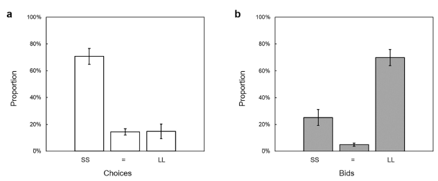
Figure 2: Proportions of (a) choosing the SS options both times (SS), choosing the SS and LL options once each (=) and choosing the LL options both times (LL); (b) bidding higher for the SS options (SS), bidding the same amount for both SS and LL options (=), and bidding higher for the LL options (LL) in Study 1. Error bars represent 95% CI.***p < 0.001.
The time preference reversals also showed changes in discount factors in both tasks. The values of k in the bid task (M = 0.04, 95% CI = [0.00, 0.08]) were significantly lower than those in the choice task (M = 0.56, 95% CI = [0.21, 0.92]), t 55 = –2.96, p = 0.005, Cohen’s d = –0.57. This result indicated that participants were more impulsive when choosing than when bidding. In summary, the above results suggested that the participants exhibited time preference reversals, thereby supporting H1.
2.2.2 Eye-tracking results
Inconsistency across bid and choice tasks
The OGPs were examined with a mixed effect linear regression, including the fixed effect of the task (1 = bid task; 0 = choice task) and the random effects of participant and item. The result showed that the participants’ OGP in the bid task was significantly greater than that in the choice task (M bid = 0.634, 95% CI = [0.629, 0.638] vs. M choice = 0.509; 95% CI = [0.505, 0.512]), b = 0.12, 95% CI = [0.10, 0.15], t = 9.38, p < 0.001. This finding indicated that participants allocated more attention on the outcome attribute in the bid task than that of the choice task (see Figure 3a).
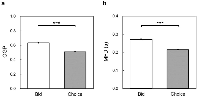
Figure 3: Results of eye-tracking measures in Study 1. (a) The OGP in the bid task is greater than that in the choice task; (b) The MFD in the bid task is greater than that in the choice task. Error bars represent 95% CI.***p < 0.001.
The MFD was also examined with a mixed effect linear regression, including the fixed effect of the task and the random effects of participant and item. The result showed that the MFD in the bid task was significantly greater than that in the choice task (M bid = 0.272 s, 95% CI = [0.269, 0.274] vs. M choice = 0.215 s, 95% CI = [0.214, 0.217]), b = 0.06, 95% CI = [0.04, 0.07], t = 9.34, p < 0.001 (see Figure 3b). The results indicated that participants’ cognitive efforts in the bid task were higher than those in the choice task.
In summary, the results of eye-tracking measures indicated that compared with the choice task, the bid task gained more fixations on the outcome attribute and obtained longer fixations, thereby supporting H2.
Mediation analysis
To further verify the relationship between eye-tracking measures and time preference reversals, the parallel multiple mediator model in MEMORE (Reference Montoya and HayesMontoya & Hayes, 2017) for SPSS was used to test the effect of task on the bids/choices through the OGP and MFD. The parallel mediation model was used to determine the correlations between the mediators and estimate the indirect effect of each mediator while controlling for the effect of others (Reference Montoya and HayesMontoya & Hayes, 2017). The task (independent variable) was entered as a dummy-coded variable (1 = bid task; 0 = choice task). Bids/choices (dependent variable) were entered as a nominal variable (–1 = bid higher for the SS options in the bid task or chose the SS options both times in the choice task; 0 = bid the same amount for both the SS and LL options in the bid task or chose the SS and LL options once each in the choice task; 1 = bid higher for the LL options in the bid task or chose the LL options both times in the choice task). The mediators were the values of OGP and MFD. Confidence intervals of 95% were generated based on 5,000 bootstrap samples.
Figure 4 shows the results of the parallel mediation analysis through the OGP and MFD on the bids/choices. Significant indirect effect of task on bids/choices was revealed through the OGP (a 1b 1 = 0.012, 95% CI = [0.007, 0.019]), whereas the indirect effect of MFD was nonsignificant (a 2b 2 = 0.01, 95% CI = [–0.03, 0.05]). The total effect of task on the bids/choices was significant (c = 1.01, 95% CI = [0.97, 1.04], p < 0.001), and the direct effect of task on bids/choices (controlling for the influence of the mediators) remained significant (c’ = 0.98, 95% CI = [0.93, 1.03], p < 0.001). This finding indicated that task still accounted for variance in the bids/choices over and above the mediation effects (see Figure 4).

Figure 4: Results of the parallel mediation analysis of OGP and MFD on bids/choices in Study 1. The indirect effect is the product of a and b. The coefficients in parentheses are the total effect (i.e., the sum of the indirect and direct effects).***p < 0.001.
As a robustness check, we separately conducted two mediation models with the values of OGP and MFD as the only mediators. The results revealed that the indirect effect of task on bids/choices through the OGP remained significant. See the supplementary materials for details.
The results revealed that the OGP (index of attention allocated to outcome attribute) significantly mediated the relation between task and bids/choices. Compared with the choice task, the bid task showed that more attention was allocated to the outcome attributes, thus leading to an increase in preference on the LL options. By contrast, the MFD (index of cognitive effort) did not significantly mediate the link between task and bids/choices. Therefore, H3 was partially supported.
2.2.3 Behavioral self-report and time preference reversals
We also examined the extent of correlation between the preference reversal in intertemporal choices and individual differences in impulsivity and maximizing tendencies.
BIS score
To examine whether task moderated the link of impulsivity and k value, we conducted linear regression on the k value with task and BIS scores as predictors. The results revealed that the interaction between task and BIS scores was non-significant (b = 0.04, 95% CI = [–0.0005, 0.08], t = 1.96, p = 0.053). Given our strong hypothesis on the interaction (H4), although no significant interaction effect existed between task and BIS scores, we performed simple effects analyses. We found that the BIS scores can predict participants’ k values in the choice task (b = 0.04, 95% CI = [0.01, 0.07], t = 2.86, p = 0.005) but not those in the bid task (b = 0.001, 95% CI = [–0.03, 0.03], t = 0.09, p = 0.926) (see Figure 5a), which is consistent with H4.
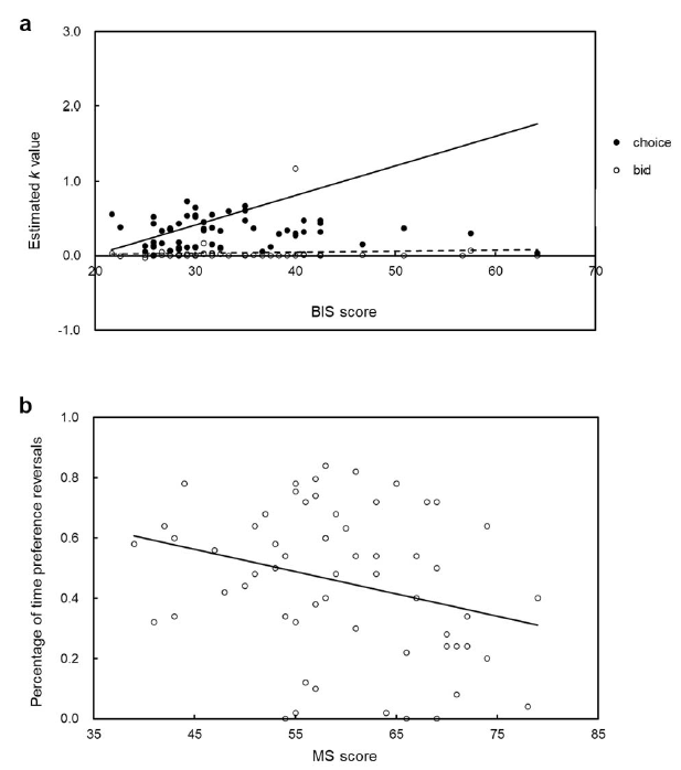
Figure 5: Results of behavioral self-report and time preference reversals in Study 1. (a) Scatter plots of the relationship between participant estimated k values and their BIS scores in both tasks; (b) Scatter plots of the relationship between the percentage of time preference reversals and MS scores. The black lines indicate identity lines.
MS score
We then examined whether the maximizing tendencies correlated with the extent of individual time preference reversals. The percentage of time preference reversals (i.e., each item was denoted as 1 if the participant chose the SS options both times in the choice task and bid higher on the LL options in the bid task; otherwise, 0; then, all items were averaged) was calculated for each participant. A linear regression revealed that the MS score was a significant predictor for the percentage of time preference reversals (b = –0.007, 95% CI = [–0.01, –0.001], t = –2.30, p = 0.025) (see Figure 5b), thereby supporting H5.
3 Study 2
To confirm the findings in Study 1 and satisfy the need for increased reproducibility in psychology research (Open-Science-Collaboration, 2015), we conducted a pre-registered replication of Study 1 via the Open Science Framework (https://osf.io/zh3s7/) with the following changes. First, the amount of information on the screen was controlled as the same in the bid and choice tasks. Second, participants could not enter their bids or choices until they finished searching the information of the options. This experimental design can isolate participants’ information searching and typing and thus eliminate the influence of typing on the eye-tracking measures. Third, the incentives were modified to avoid potential effect of scaling down the delays/outcomes on how the delays were responded. In Study 2, one of the participants would be randomly selected and would be paid the option they selected on a random trial for each task. Fourth, the order of completing the bid/choice tasks and the personality scales was counterbalanced across participants. Finally, each pair of options was presented once during choice trials in Study 2. In Study 1, each pair of options was repeated twice, which may lead to different definitions of preference reversals (Reference Alós-Ferrer, Jaudas and RitschelAlós-Ferrer et al., 2021).
3.1 Method
3.1.1 Participants
Considering that the results concerning correlations with personality factors typically need a relatively large sample size, we conducted the power analysis on the basis of the results of personality factors in Study 1. G∗Power (Reference Faul, Erdfelder, Lang and BuchnerFaul et al., 2007) is used to calculate the required number of participants to achieve 80% power and detect an effect size of Cohen’s f = 0.077 (the smallest effect size based on the results of personality factors in Study 1) at the standard 0.05 alpha error probability using a linear regression. The required sample size was N = 104. A total of 110 college students (59% female, M age = 21.0 ± 2.2) were recruited as participants in the current study. Participants received 35 yuan (RMB; approximately US$5.3) in cash for participation, and two participants received the additional reward. All participants had normal or corrected-to-normal vision and provided written informed consent prior to the experiment. Approval for the study was obtained from the university institutional review board.
3.1.2 Experimental task
Similar to Study 1, participants completed the choice and bid tasks in the experiment. In the choice task, participants indicated their preference between a pair of SS and LL options. A total of 50 pairs of options were presented. In the bid task, the same 50 pairs of options were presented on the screen, and participants were requested to indicate their exact valuation of the intertemporal options.
The 50 pairs of options were the same in Study 1, and each pair of options was presented once in the two tasks. Similar to Study 1, the orders of tasks and placement of attributes (i.e., delay or outcome) were counterbalanced across participants. The options were presented in randomized order for each participant in each decision format.
To further incentivize their cooperation, the participants were informed that at the end of the experiment, one of the participants would be randomly selected for each task and would be paid the option they selected on a random trial. If a choice trial was selected, the participant was paid according to his/her decision on that trial and received a real delayed reward. If a bid trial was selected, the participant was paid using the Becker–DeGroot–Marschak method (Reference Becker, DeGroot and MarschakBecker et al., 1964).
3.1.3 Procedure
Upon entering the laboratory, participants received general instructions regarding the experiment and were asked to sign the informed consent. The chair was adjusted to ensure participant comfort. A 5-point calibration and validation procedure was used. The maximum error of validation was 0.5 degrees in the visual angle. In both tasks, two practice trials were first presented to familiarize the participants with the experiment procedure.
During a choice trial, a fixation disc appeared at the center of the screen. The disc also served as a drift check for the eye tracker. When fixation was registered, the participants pressed the space key to view the options. After viewing the options, the participants pressed the space key and the words, “Choose Now,” were shown at the center of the screen. Participants had unlimited time to choose between the two options, pressing “F” to choose the option on the left or “J” to choose the option on the right. After participants submitted their responses, a feedback with a check mark on the side of the chosen option was presented for 1,000 ms. See Figure 6a.
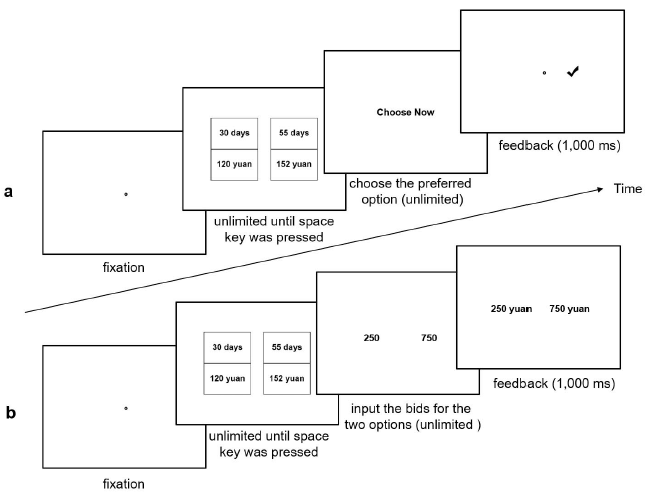
Figure 6: Trial procedure and timing in (a) the choice task and (b) the bid task in Study 2.
During a bid trial, a fixation disc appeared at the center of the screen. The disc also served as a drift check for the eye tracker. When fixation was registered, the participants pressed the space key to view the options. After viewing the options, the participants pressed the space key and the options disappeared. Participants had unlimited time to input their bids for the two intertemporal options using a keyboard and to submit their response by pressing the “Enter” key. Submitted bids were considered final, and a feedback with the amounts of bids was presented for 1,000 ms. See Figure 6b.
Similar to Study 1, the participants were asked to complete two questionnaires, the MS and BIS. The order of completing the bid/choice tasks and the questionnaires was counterbalanced across participants. Half of the participants completed the bid/choice tasks first, whereas the other half completed the questionnaires first.
3.1.4 Data analysis
Preprocessing of eye-tracking data
Eye-movement data were analyzed using the EyeLink Data Viewer. Fixations were defined as periods of a relatively stable gaze between two saccades, but fixations shorter than 50 ms were excluded from the analyses. In the choice and bid tasks, four non-overlapping, identically sized (10.8∘ × 7.7∘ visual angle) rectangular ROIs around each piece of information were defined.
Participants’ k values were estimated using the same method with Study 1. Data from seven participants were not convergent, thereby excluding their k values from the discount factor analysis.
3.2 Results
3.2.1 Behavioral results
Response time
Response times (the total amount of time a participant spent before pressing the space key) were examined with a mixed-effect linear regression including the fixed effect of the task (1 = bid task; 0 = choice task) and the random effects of participant and item. We found that on average, bidding required significantly longer time than making a choice (M bid = 15.10 s, 95% CI = [14.80, 15.40] vs. M choice = 4.73 s, 95% CI = [4.63, 4.82]; b = 10.39, 95% CI = [9.26, 11.52], t = 17.99, p < 0.001), which is consistent with Study 1.
Time preference reversals
For each pair of options, responses were categorized in the choice task according to whether the participants chose the SS option (“SS”) or the LL option (“LL”). In the bid task, responses were categorized according to whether the participants bid higher on the SS option (“SS”), bid equal amounts for both options (“=”), or bid higher on the LL options (“LL”). The proportions of each category were calculated for each participant.
Similar to Study 1, the results revealed a time preference reversal effect. In the choice task, the proportions of choosing LL options (M = 26.5%, 95% CI = [22.4%, 30.7%]) were significantly lower than 50% (t 109 = –11.23, p < 0.001, Cohen’s d = –1.07) (See Figure 7a). By contrast, in the bid task, the proportions of bidding higher on the LL options (M = 58.4%, 95% CI = [53.5%, 63.2%]) were significantly higher than 50% (t 109 = 3.41, p < 0.001, Cohen’s d = 0.33) (See Figure 7b). Participants preferred the LL options significantly more often when bidding than when choosing, t 109 = 11.51, p < 0.001, Cohen’s d = 1.33.

Figure 7: Proportions of (a) choosing the SS options (SS) and choosing the LL options (LL); (b) bidding higher for the SS options (SS), bidding the same amount for both the SS and LL options (=), and bidding higher for the LL options (LL) in Study 2. Error bars represent 95% CI.***p < 0.001.
The time preference reversals also showed changes in discount factors in both tasks. The values of k in the bid task (M = 0.04, 95% CI = [0.02, 0.08]) were significantly lower than those in the choice task (M = 0.85, 95% CI = [0.41, 1.28]; t 102 = –3.58, p < 0.001, Cohen’s d = –0.51). This result indicated that participants were more impulsive when choosing than when bidding.
In summary, the above results suggested that the participants exhibited time preference reversals, replicating the results in Study 1.
3.2.2 Eye-tracking results
Inconsistency across bid and choice tasks
The OGPs were examined with a mixed effect linear regression, including the fixed effect of the task and the random effects of participant and item. The result showed that the participants’ OGP in the bid task was significantly greater than that in the choice task (M bid = 0.628, 95% CI = [0.624, 0.633] vs. M choice = 0.507; 95% CI = [0.503, 0.512]; b = 0.12, 95% CI = [0.10, 0.14], t = 10.00, p < 0.001). This finding indicated that participants allocated more attention on the outcome attribute in the bid task than that of the choice task (see Figure 3a).
The MFD was also examined with a mixed effect linear regression, including the fixed effect of the task and the random effects of participant and item. The result showed that the MFD in the bid task was significantly greater than that in the choice task (M bid = 0.278 s, 95% CI = [0.276, 0.280] vs. M choice = 0.217 s, 95% CI = [0.216, 0.218]; b = 0.06, 95% CI = [0.05, 0.07], t = 15.33, p < 0.001) (see Figure 3b). The results indicated that participants’ cognitive efforts in the bid task were higher than those in the choice task.
In summary, the results of eye-tracking measures indicated that compared with the choice task, the bid task gained more fixations on the outcome attribute and obtained longer fixations, replicating the results in Study 1.

Figure 8: Results of eye-tracking measures in Study 2. (a) The OGP in the bid task is greater than that in the choice task; (b) The MFD in the bid task is greater than that in the choice task. Error bars represent 95% CI.***p < 0.001.
Mediation analysis
Similar to Study 1, we conducted the mediation analysis to test the effect of task on the bids/choices through the OGP and MFD. The task (independent variable) was entered as a dummy-coded variable (1 = bid task; 0 = choice task). Bids/choices (dependent variable) were entered as dummy-coded variables (0 = bid higher for the SS options in the bid task or chose the SS options in the choice task; 1 = bid higher for the LL options in the bid task or chose the LL options in the choice task). The mediators were the values of OGP and MFD. Confidence intervals of 95% were generated based on 5,000 bootstrap samples.
Figure 9 shows the results of the parallel mediation analysis through the OGP and MFD on the bids/choices. Significant indirect effect of task on bids/choices was revealed through the OGP (a 1b 1 = 0.034, 95% CI = [0.024, 0.043]), whereas the indirect effect of MFD was nonsignificant (a 2b 2 = –0.011, 95% CI = [–0.024, 0.003]). The total effect of task on the bids/choices was significant (c = 0.34, 95% CI = [0.33, 0.36], p < 0.001), and the direct effect of task on bids/choices remained significant and essentially unchanged (c’ = 0.32, 95% CI = [0.30, 0.34], p < 0.001). This finding indicated that task still accounted for variance in the bids/choices over and above the mediation effects (see Figure 9).

Figure 9: Results of the parallel mediation analysis of OGP and MFD on bids/choices in Study 2. The indirect effect is the product of a and b. The coefficients in parentheses are the total effect.***p < 0.001
Similar to Study 1, as a robustness check, we separately conducted two mediation models with the values of OGP and MFD as the only mediators. The results revealed that the indirect effect of task on bids/choices through the OGP remained significant. See the supplementary materials for details.
The results of mediation analysis replicated the findings in Study 1. The OGP significantly mediated the relation between task and bids/choices. Compared with the choice task, the bid task showed that extra attention was allocated to the outcome attributes, thus leading to an increase in preference on LL options. By contrast, the MFD did not significantly mediate the link between task and bids/choices.
3.2.3 Behavioral self-report and time preference reversals
Similar to Study 1, we examined the correlation between the time preference reversal and individual differences in impulsivity and maximizing tendencies.
BIS score
To examine whether task moderated the link of impulsivity and k value, we conducted linear regression on the k value with task and BIS scores as predictors. The results revealed that the interaction between task and BIS scores was non-significant (b = 0.002, 95% CI = [–0.035, 0.040], t = 0.14, p = 0.890) (see Figure 10a). Simple effects analyses showed no significant effect, which is inconsistent with Study 1.
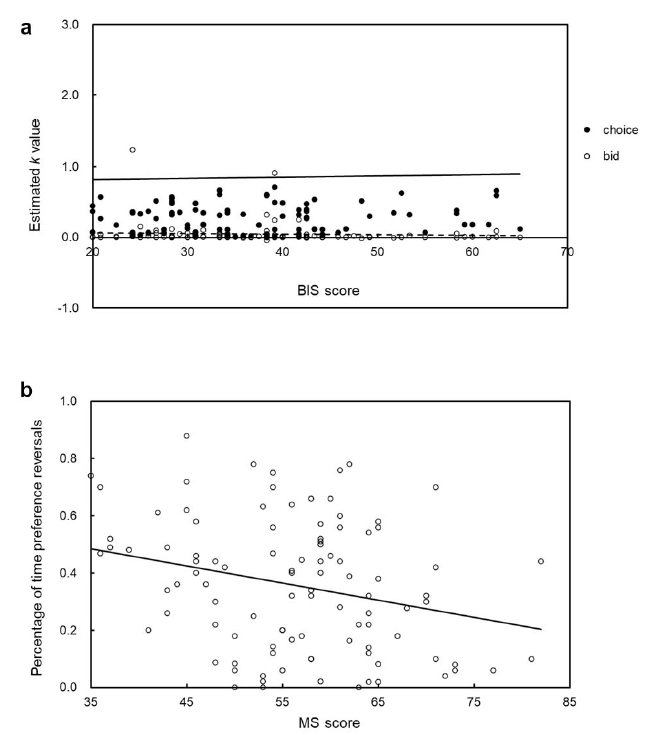
Figure 10: Results of behavioral self-report and time preference reversals in Study 2. (a) Scatter plots of the relationship between participant estimated k values and their BIS scores in both tasks; (b) Scatter plots of the relationship between the percentage of time preference reversals and MS scores. The black lines indicate identity lines.
MS score
We then examined whether the maximizing tendencies correlated with the extent of individual time preference reversals. A linear regression revealed that the MS score was a significant predictor for the percentage of time preference reversals (b = –0.006, 95% CI = [–0.009, –0.002], t = –3.39, p < 0.001) (see Figure 10b), replicating the results in Study 1.
4 Discussion
The present study replicated the time preference reversal in a wide range of intertemporal options. In the two studies, we replicated the time preference reversal in which individuals facing a pair of intertemporal options choose the SS option but assign a higher value to the LL option. From a pair of intertemporal options, the participants chose the SS option most of the time (71% in Study 1 and 74% in Study 2) but assigned higher prices to the LL option most of the time (70% in Study 1 and 58% in Study 2). Consistent with these results, participants were generally impatient when choosing and were relatively patient when bidding. The preference reversals were previously established in risky choice (Reference Grether and PlottGrether & Plott, 1979; Reference Kim, Seligman and KableKim et al., 2012; Reference Lichtenstein and SlovicLichtenstein & Slovic, 1971, 1973), and the present results provided evidence for the robustness of preference reversals in intertemporal choice. These findings suggested a universal preference gap between elicitations of choices and bids in different decision domains.
The eye-tracking results in both studies were consistent with the contingent weighting hypothesis (Reference Mellers, Ordoñez and BirnbaumMellers et al., 1992; Reference Tversky, Sattath and SlovicTversky et al., 1988) that time preference reversals result from an increased weight on delay attribute in value assessments during choices and a corresponding increased weight on outcome attribute during bids. The results revealed that the OGP in the choice task was greater than that in the bid task. Thus, time preference reversals may be caused by the choice and bid tasks eliciting different levels of attention allocation on outcome or delay attributes, which indicated differential weighting of attributes. The mediation analyses also showed that the greater attention was allocated to the outcome attribute, the LL options were more likely to be preferred/bid higher. This finding indicated that an individual’s weight on outcome attribute is related to his/her patience. Previous research manipulated participants to gaze longer on the outcome/delay attribute and found that gazed longer attribute mediated the effect of the manipulation on the choice (Reference Sui, Liu and RaoLiu et al., 2020). Their mediation analyses suggested that when manipulating a participant to gaze longer at the outcome attribute, then, the preference for the LL option would increase. It is thus inferred that this attribute-based gaze time plays a crucial role in the process of time preference. Remarkably, the mediation effect found in our studies is relatively small, which is consistent with previous research (Reference Sui, Liu and RaoLiu et al., 2020). This finding implies that the OGP cannot sufficiently explain the underlying mechanisms of time preference reversal. Future studies may further explore the process of time preference reversal.
The eye-tracking results also presented implications to the strategy compatibility hypothesis (Reference Stalmeier, Wakker and BezembinderStalmeier et al., 1997), in which individuals tended to use the intuitive strategy in the choice task and use the deliberate strategy in the bid task, leading to varied cognitive efforts. The results of the two studies revealed that the MFD in the choice task was shorter than that in the bid task, which is consistent with the strategy compatibility hypothesis. In Study 1, participants were asked to type the answer when searching the information of intertemporal options. The bid task needs more typing than the choice task, and typing usually causes longer fixations than silent reading (Reference RaynerRayner, 1998), which may explain the difference in MFD in Study 1. However, in Study 2, we isolated participants’ information searching and typing. Participants could not enter their bids or choices until they finished searching the information of the options. We found that the MFD in the choice task was still shorter than that in the bid task, which is consistent with Study 1. These results suggest that participants exerted more cognitive effort during the information searching in the bid task than in the choice task.
The mediation analyses revealed that the MFD did not significantly mediate the link between task and bids/choices. The finding indicated that although the choice/bid tasks lead to varied MFDs (Reference Amblee, Ullah and KimAmblee et al., 2017; Reference Holmqvist, Nyström, Andersson, Dewhurst, Jarodzka and Van deWeijerHolmqvist et al., 2011), the variations could not explain the differences in the bids/choices. In other words, the more cognitive effort exerted in the choice/bid tasks does not mean that the LL options were more likely to be preferred/bid higher. Therefore, the nonsignificant mediation effect of MFD actually did not contradict the prediction of the strategy compatibility hypothesis.
The results of the correlation between behavioral self-report and time preference reversals revealed that the scores of maximizing tendencies could negatively predict participants’ extent of time preference reversals. That is, high scores on the measure of maximizing tendencies indicated a strong likelihood of participants adopting the deliberate maximizing strategy (Reference SchwartzSchwartz, 2015; Reference Schwartz, Ward, Monterosso, Lyubomirsky, White and LehmanSchwartz et al., 2002), thereby leading to lower proportions of time preference reversals. From the two studies, we confirmed the robustness of the relationship between maximizing tendencies and time preference reversals. This finding coordinated with the strategy compatibility hypothesis.
We also examined whether the task moderates the link between the individual differences in impulsivity and participants’ discounting rates. Given that participants tended to apply the intuitive strategy in the choice task than in the bid task and the impulsivity could be more likely to affect the intuitive strategy (Reference Glimcher, Kable and LouieGlimcher et al., 2007; Reference Ripke, Hubner, Mennigen, Muller, Rodehacke, Schmidt, Jacob and SmolkaRipke et al., 2012), the scores of impulsivity scale are thus assumed to possibly predict participant discounting factors in the choice task but not in the bid task. In Study 1, although the interaction effect between task and BIS scores was nonsignificant, simple effects analyses revealed that the BIS scores can predict participants’ k values in the choice task but not those in the bid task. However, this result was not replicated in the pre-registered Study 2 with a larger sample. A post hoc observation revealed the prevalence of low k values for high BIS scores in Figure 5a, implying that the fitted linear model is not a particularly good characterization of the relationship between BIS scores and k values.
Although substantial research examined the cognitive processes of preference reversal in risky choice (Reference Alós-Ferrer, Jaudas and RitschelAlós-Ferrer et al., 2021; Reference Ashby, Yechiam and Ben-EliezerAshby et al., 2018; Reference Kim, Seligman and KableKim et al., 2012; Reference Rubaltelli, Dickert and SlovicRubaltelli et al., 2012), to our knowledge, the current work is the first research to investigate the cognitive processes of this phenomenon in intertemporal choice. Previous studies revealed that individuals gaze longer on the probability attribute in the choice task but gaze longer on the outcome attribute in the bid task (Reference Ashby, Yechiam and Ben-EliezerAshby et al., 2018; Reference Kim, Seligman and KableKim et al., 2012). Moreover, individuals exhibited longer fixations in the bid task (Reference Rubaltelli, Dickert and SlovicRubaltelli et al., 2012) than that in the rating task. Our findings are consistent with those of previous studies on risky choice. These convergences suggested that visual attention played an important role in preference reversal and may lead to improved understanding of their mechanisms. From the two eye-tracking experiments, the present research provided supportive evidence for both contingent weighting hypothesis and strategy compatibility hypothesis. Although the two hypotheses may compete with each other, they are not altogether mutually exclusive. If we allow for the possibility that different people have learned to deal with delay rewards in different ways, we will probably find some individuals tending to behave according to one hypothesis, whereas others may be better represented by the other kind of explanation.
Finally, we acknowledge that this study has limitations. First, the intertemporal options used in our experiment only involved gains. Future studies should consider examining the time preference reversals in a loss frame. An asymmetry between gain and loss frames was previously observed in intertemporal choices (Reference Sun, Li, Chen, Zhao, Rao, Liang and LiSun et al., 2015; Reference ThalerThaler, 1981), and the relationships between visual attention and loss sensitivity varied in choice and valuation tasks (Reference Ashby, Yechiam and Ben-EliezerAshby et al., 2018). Therefore, there might be an asymmetry between gain and loss frames in time preference reversals. Second, the method for estimating k values in the bid task can be improved in future studies. Following previous research (Reference Kim, Seligman and KableKim et al., 2012), we used least squares to estimate each participant’s k value in the bid task. This method was applied on the basis of the assumption that participant’s bid equals the discounted value of the intertemporal option, and this assumption may not be warranted in certain situations. Future studies can develop new methods to make a more precise estimate of individual’s discount factor in the bid task. For instance, the instructions can be modified to ask the participants to indicate their discounted values of the intertemporal options instead of the bids or prices. Third, when examining whether individuals exhibit time preference reversals, the mean values were presented and thus consequently missed the variability in individual difference. We can see the individual difference in time preference reversals from Figures 5a and 10a. Future research may further identify the contributing factors and boundary conditions of time preference reversal. For example, the effect of the properties of the intertemporal options, such as the magnitude of the outcomes, can be explored in the future.
In summary, the two experiments enabled us to replicate the time preference reversal phenomenon and found that the reversals were accompanied by different visual degrees of attention to the outcome attribute and fixation duration. In addition, individuals’ maximizing tendencies can negatively predict their time preference reversals. The findings provided an improved theoretical understanding of the potential mechanisms and processes involved in time preference reversals.


 Open access