


I. Introduction
Diverse research relies on the ratings that critics, judges, and consumers assign to wines. Recent examples include Gergaud, Ginsburg, and Moreno-Ternero (Reference Gergaud, Ginsburgh and Moreno-Ternero2021) method of aggregating judges’ ratings; Hölle et al. (Reference Hölle, Aufschnaiter, Bogon, Pfeuffer, Kiesel and Thomaschke2020) finding that customers’ ratings of wines online can vary due to screen position alone; Corsi and Ashenfelter (Reference Corsi and Ashenfelter2019) analysis of the correlation between weather data and ratings; Capehart (Reference Capehart2019) analysis of whether or not training improves the accuracy of ratings; Lam et al. (Reference Lam, Lambrechts, Pitt and Afsharipour2019) analysis of how ratings affect written reviews; and Malfeito-Ferreira, Diako, and Ross (Reference Malfeito-Ferreira, Diako and Ross2019) identification of the sensory and chemical differences between grand-gold and gold rated wines. In addition to such research, numerous critics, competitions, clubs, and vendors use ratings to compare wines, convey information, and sell wine.
This short article focuses on a difficulty with wine ratings for the uses previously noted that is due to the finding that each rating observed is one drawn from a latent distribution that is wine- and judge-specific. What can be deduced about the shape of a latent distribution from one observation? Section II summarizes research showing that the ratings that critics and judges assign are stochastic, heteroscedastic, and may be affected by anchoring, expectations, and serial position biases. Section III shows that those conditions lead to a problem that is inverse, ill-posed with a sample size of one, and partially or wholly categorical rather than cardinal. A maximum entropy solution to that problem is posed in Section IV for sample sizes of zero, one, a few blind replicates, and many observations. An example is presented in Section V, and the results are consistent with the actual distributions observed for ratings assigned to blind replicates. An application to tasting data with blind triplicates published by Cicchetti (Reference Cicchetti2014) in Section VI shows that the approach proposed has less than 25% of the error in analyses of observed ratings alone. Conclusions follow in Section VII.
II. The maelstrom about a rating observed
Judges assign ratings to wines that are within a bounded set of scores or an ordered set of categories, or a set of ranks. Examples of scores include the 50- to 100-point scales used by Wine Advocate and Wine Spectator, UC Davis’ 0 to 20-point scale, Jancis Robinson's 12- to 20-point scale, and the 0- to 100-point scale prescribed by the International Organization of Wine and Vine (OIV). Examples of categories include the Wine & Spirit Education Trust's (WSET) six categories of quality (faulty, poor, acceptable, good, very good, and outstanding) and the California State Fair Commercial Wine Competition's (CSF) six or ten medals.Footnote 1 Further, some systems are forced rankings. If there are six wines in a flight, a judge must rank all six in order of relative preference. Liquid Assets and San Francisco FOG are examples of tasting groups that employ that approach. See reviews and comparisons of rating systems in Cicchetti and Cicchetti (Reference Cicchetti and Cicchetti2014), Kliparchuck (Reference Kliparchuck2013), and Veseth (Reference Veseth2008).
Although tasters focus on the wine in the glass, much research shows that the ratings that tasters assign are affected by other factors. Some of the factors are supported by literature that is cited later. Other factors described are reported as anecdotal and, when no literature is cited, those other factors are intended as hypotheses that remain to be tested.
A. Stochastic ratings
First, although wine ratings are not merely random, evidence that ratings are stochastic is abundant in the wine-related academic literature and trade press. Bodington (Reference Bodington2017, Reference Bodington2020) summarizes and cites four experiments with blind replicates, more than 20 other evaluations that find uncertainty in ratings, and two texts that explain the neurological, physiological, and psychological reasons for variance in the ratings that the same judge assigns to the same wine. The stochastic nature of wine ratings is not unique. Kahneman, Sibony, and Sunstein (Reference Kahneman, Sibony and Sunstein2021, pp. 80–86, 215–258) describe variance in wine ratings and in many other areas of human judgment including physicians’ diagnoses, forensic experts’ fingerprint identifications, and judges’ sentencings of criminals.
The wine-related literature cited supports several findings. A rating observed is one drawn from a latent distribution; it is one instance of, in some cases, many potential instances. Ratings are heteroscedastic, so the distribution of ratings on a wine is wine- and judge-specific, and different judges’ ratings on the same wine are not identically distributed (ID). Some judges assign ratings more consistently than others, and some wines are more difficult to rate consistently than others. Research attempts to predict ratings from physiochemical properties have struggled to obtain statistical significance. Experiments with blind replicates show that, on average, the standard deviation of the rating that the same judge assigns to the same wine within a flight is approximately 1.3 out of 10 potential rating categories. And while some judges independently assign ratings that correlate well with each other, about 10% of CSF judges assign ratings that are indistinguishable from random assignments.
Although most ratings are assigned by judges prior to any discussion of the subject wines, pre-rating discussion sometimes occurs among panelists, and some competitions require an initial rating, then discussion, and then a post-discussion rating. According to Taber (Reference Taber2005, pp. 300–301), discussion of the wines took place during the tasting at the 1976 Judgment of Paris. The CSF is an example of a competition in which judges assign an initial rating, discuss the wines with other judges, and then assign another post-discussion rating. Both sets of ratings are reported to CSF officials, and the author is not aware of any correlation or other comparisons made by the CSF. Judges can influence each other, so post-discussion ratings may not be statistically independent (I). When combined with the heteroscedasticity, post-discussion ratings may therefore not obtain the statistical ideal of independent and identically distributed (IID) observations.
B. Anchoring, expectation, and serial position biases
The score-based rating systems noted previously also assign categories of quality or award to score thresholds and ranges. For example, the OIV system sets score thresholds for Bronze, Silver, and Gold medals at scores of 80, 85, and 90, respectively.Footnote 2 With a sample of 8,400 ratings, Bodington and Malfeito-Ferreira (Reference Bodington and Malfeito-Ferreira2017) showed spikes in the frequencies of scores assigned just below those thresholds. Thus, some judges appear to anchor at OIV's category thresholds.
In addition to anchoring scores to category thresholds, there is anecdotal evidence of sequential anchoring. In a taste-and-score sequential protocol, a judge may assign a rating to the first wine and then rate the remaining wines “around” that anchor. A lag structure may also exist in which a judge rates around some composite of the most recent wines. The upper and lower bounds on ratings, whether numerical or categorical, may then merely bound a judge's assessments of relative preference.
Much research shows that judges’ expectations affect the ratings they assign. Ashton (Reference Ashton2014) found that judges assigned higher ratings to wines from New Jersey when told the wines were from California and lower ratings to wines from California when told the wines were from New Jersey. On that evidence, regardless of actual quality, an expectation of good quality may lead to a central tendency in ratings within whatever range of scores or categories indicates good quality. In addition, information provided about wines may alter expectations and ratings. For example, the pre-printed forms provided to CSF judges list the grape variety, vintage, alcohol by volume, and residual sugar of a wine next to spaces where the judge writes in a comment and then a rating.Footnote 3 Whether or not such judgments should be represented as “blind” is open to debate. Whether or not having that information affects judges’ ratings remains to be tested.
Some critics and competitions employ a sequential, step-by-step, or taste-and-rate protocol. A critic or judge tastes a wine and assigns a rating, then tastes the next wine and assigns a rating to that wine, and so on. The Judgment of Paris, the CSF, and many publishing critics employ a sequential protocol.Footnote 4 The possibility that ratings assigned during taste-and-rate protocols are affected by serial position, rather than the intrinsic qualities of the wines and judges, is difficult to assess and rule out. Serial position bias may occur in wine competitions due to palate fatigue, rest breaks, meal breaks, physiological, and psychological factors.Footnote 5 There are anecdotal reports from judges who say there is temptation to assign a high rating to a dry and high-acid wine because it is refreshing in a sequence just after several off-dry and alcoholic wines. UC Davis’ class for potential wine judges warns of position bias affecting differences in ratings due to the sequence of wines, breaks, and lunch.Footnote 6 Filipello (Reference Filipello1955, Reference Filipello1956, Reference Filipello1957) and Filipello and Berg (Reference Filipello and Berg1958) conducted various tests using sequential protocols and found evidence of primacy bias. Mantonakis et al. (Reference Mantonakis, Rodero, Lesschaeve and Hastie2009, p. 1311) found that “high knowledge” wine tasters are more prone than “low knowledge” wine tasters to primacy and recency bias. The sequence of wines tasted at the 1976 Judgment of Paris has never been disclosed, so what effect position bias may have had on the results remains unknown.Footnote 7
Standing back, within the maelstrom described earlier, what can be deduced about a rating observed? A rating is a discrete score, ordered category, or rank drawn from a bounded set. A rating is stochastic, and a rating observed is one drawn from a wine- and judge-specific distribution. And that rating observed may have been affected by anchoring, expectation, and/or serial position biases.
III. The problem with one observation
Except for rare experiments with blind replicates in a flight, critics and judges examine one wine (or each wine in a flight) and then assign one rating to that wine (or one rating to each wine in a flight). That is an acute problem. Literature cited previously shows that ratings are heteroscedastic, ratings are not ID, and they may not be IID, so neither the collection of all judges’ ratings on a wine nor the collection of one judge's ratings on other wines can be employed to estimate the distribution of potential ratings by one judge on one wine. Each distribution is unique, and only one sample drawn from that distribution is observed.
Score increments are usually whole numbers; some competitions allow half-points, so even score assignments are discrete. The scores, category choices, and ranks used by critics and allowed by competitions are bounded sets. Although a rating is observed after it is assigned by a judge, aside from being discrete and bounded, no other information about the distribution of that rating is observed. Estimating the shape of the discrete and bounded distribution is thus an inverse problem. The shape and any parameters describing that shape must be inferred from the observation. And, unless the shape of the distribution can be defined by one parameter, the problem is ill-posed. If ill-posed, there are more unknown parameters than observations, so a unique distribution cannot be defined.
There is another difficulty. Although scores appear to be cardinal, the anchoring behaviors described earlier indicate that some judges mix the notions of cardinal scoring and ordered categories. On that basis, treating scored ratings as cardinal appears perilous. And trying to construct a model of a judge's scoring behavior, at minimum, exacerbates the inverse and ill-posed aspects of the problem.
The problem of what can be deduced about the shape of a latent distribution from one observation is not new. Several authors have examined what can be inferred about continuous and symmetric distributions; see Casella and Strawderman (Reference Casella and Strawderman1981), Rodriguez (Reference Rodriguez, Skilling and Sibisi1996), Golan, Judge, and Miller (Reference Golan, Judge and Miller1996), Leaf, Hui, and Lui (Reference Leaf, Hui and Lui2009), and Cook and Harslett (Reference Cook and Harslett2015). Their methods are summarized in Appendix A, and the discussion that follows focuses on what can be inferred from one observation about a bounded, discrete, ordinal scale, and probably asymmetric distribution.
IV. A maximum entropy solution to an inverse and ill-posed problem
Hartley (Reference Hartley1928) and Shannon (Reference Shannon1948) posed the notion that uncertainty about something—in this case, a judge's rating on a wine—can be expressed as information entropy. The higher the entropy, the higher the uncertainty. Jaynes (Reference Jaynes1957a, Reference Jaynes1957b) then proposed the idea that a distribution that maximizes entropy assumes the least precision in what is known about the latent distribution of the data. When there are not enough data to estimate a unique parameter, set that parameter to maximize entropy so that you do not pretend to know more than you actually do. This maximum entropy approach is often employed to solve inverse and ill-posed problems. See, for example, Golan, Judge, and Miller (Reference Golan, Judge and Miller1996, pp. 7–10 in particular).
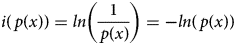
Shannon (Reference Shannon1948) defined the amount of information (i) in a random variable (x), in Equation (1), as the logarithm of the inverse of its probability (p). Building on that, he expressed information entropy (H) in Equation (2) as the expectation of information about a random variable. While the precise meaning of information entropy is controversial, H is highest for a uniform random distribution and lowest for a single-point, degenerate distribution. The informational difference (I) between two distributions, p and q, known as cross-entropy, appears in Equation (3).Footnote 8 See Rioul (Reference Rioul2008) and Lombardi, Holik, and Vanni (Reference Lombardi, Holik and Vanni2016) for histories and discussions of these famous results.

Applying Jaynes’ notion of maximum entropy to none, one or more observations (x o) drawn from a discrete and bounded but unknown distribution ($\hat{p}$ ) yields the solution proposed in Equation (4). A derivation of Equation (4) appears in Appendix B. The first term $I( {u, \;\hat{p}} )$
 is the cross-entropy between $\hat{p}$
 and a uniform random distribution (u). The second term $I( {q\vert x^o, \;\hat{p}} )$
 is cross-entropy between $\hat{p}$
 and the distribution that is observed, (q|x o). If n = 0 then the minimization in Equation (4) is a dual of the maximum entropy solution u(all x) = 1/(max − min + 1).Footnote 9 If n = 1 then q is a one-hot vector where q(x o) = 1. For n = 3, q could be the distribution observed for blind triplicates. As n → ∞ then $\hat{p}$
 tends to the distribution implied by a large sample and the influence of the random distribution, u, tends to zero.Footnote 10 That minimization is the dual of the maximum likelihood solution for a large sample. See Golan, Judge, and Miller (Reference Golan, Judge and Miller1996, pp. 25, 41) and Shashua (Reference Shashua2008, p. 3–3) regarding the duality of maximum likelihood and minimum entropy.

Among many potential probability mass functions (PMFs) for $\hat{p}$ , a simple one is a categorical distribution that is discrete, bounded (min, max), and has a probability for every potential rating. That PMF has max – min + 1 = R unknown probabilities to estimate. For just one observation x o, the maximum entropy solution to Equation (4) for R = 10 is p(x = x o) = 0.55 and p(all x ≠ x o) = 0.05. That spikey solution is not very credible. It ignores the notion of central tendency. It ignores the evidence cited in Section II that while most judges may not assign the exact same ratings to replicates in a flight, the ratings they do assign tend to cluster around nearby scores, categories, or ranks.
Central tendency and clustering are notions about frequency and distance. Distance is easily expressed on a cardinal scale of scores, but the evidence cited in Section II shows that score assignments may be influenced by ordinal considerations, and many rating systems are ordered categories alone. The difficulty with mapping ordinal categories to a cardinal scale is that, although categories may be adjacent, there is no information about the widths of categories or the transitions between categories. And if scores are interpreted as expressions of economic utility, the economics literature summarized in Barnett (Reference Barnett2003, p. 41) is rich in what he calls the modern view that utility is ordinal, cannot be employed to calculate indifference points between goods, and cannot be employed to compare one person to another. Marks (Reference Marks2019) draws similar conclusions in his analysis of wine ratings as on hedonic scales. While using ratings to make inferences about interpersonal utility and indifference points may violate the logic of utility theory, statistical analysis of ordinal ratings for other purposes is common. According to Chen and Wang (Reference Chen and Wang2014), ordinal data are the most frequently encountered type of data in social science.Footnote 11 Chen and Wang review methods of mapping categorical responses to numerical values, and those methods include merely ranking the categories. In their texts concerning analysis of categorical data, Agresti (Reference Agresti2007, pp. 43–44, 119, 195, 230, 299) and Lynch (Reference Lynch2007, p. 219) discuss methods of mapping that again include ranking, and they also present PMFs with dispersion parameters to describe central tendency and clustering in the distributions of categorical data.
Although the research cited previously explains several methods of mapping categorical data to numerical values and several PMFs, this article does not pursue finding a “best” method of mapping and/or the best PMF. The best of those probably depends on the form of the rating data and the intended analysis or hypothesis test. Before moving forward to an example and a test, Equation (4) is not an assertion that the distribution of a judge's potential ratings on a wine is nearly random for small sample sizes. It is an assertion that evident knowledge about that distribution, for a small sample, can only support a distribution that is a little better than random.
V. An example
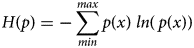
Suppose in this example that a judge assigns a rating of “Gold–” to a wine entered in a competition with ten ordered categories of rating: No Award, Bronze–, Bronze, Bronze+, Silver-, Silver, Silver+, Gold–, Gold, and Gold+. In that case, and mapping from categories to ranks, x 0 = 8 ∈ (1, 10). Suppose further that the latent distribution of that rating can be described by a discrete and bounded Gaussian function of mean (μ) and variance (σ 2). With emphasis, the intent is to describe the distribution of potential ordinal ratings assigned by one judge to one wine and there is no intent to make any inference about economic utility or to make a comparison with any other wine or judge. Knowing only that x 0 = 8 ∈ (1, 10) and using Equation (4), the maximum-entropy estimate of the latent distribution of that rating observed appears as the dashed line in Figure 1. The stair-step shape of the distribution reflects the discrete categories. Next, the evidence cited in Section II shows that the standard deviation (SD) in ratings assigned by trained and tested CSF wine judges to blind triplicates averages approximately 1.3 out of 10 ratings; σ = 1.3. Using that estimate of SD and Equation (4), the maximum-entropy estimate of μ yields the distribution that appears as the solid line in Figure 1. MATLAB code for Figure 1 is available on request.
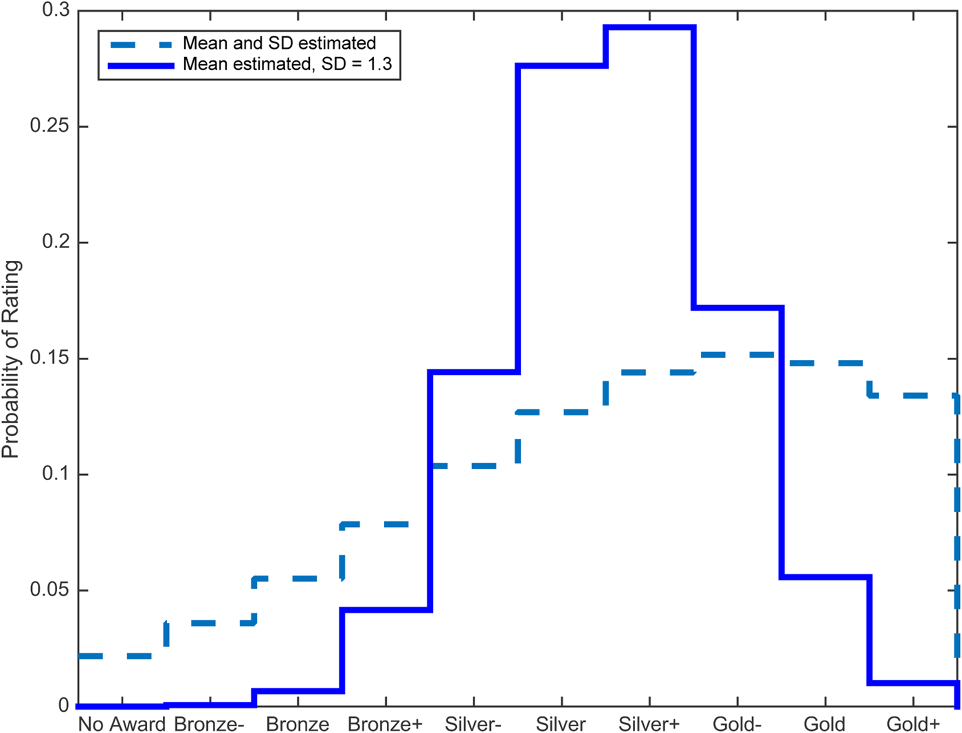
Figure 1. Estimated probability distributions of one observed rating of “Gold-”.
The results in Figure 1 are consistent with the maximum entropy findings for continuous and unbounded distributions summarized in Appendix A. With only one observation, results tend toward a random distribution because that reflects knowing the least information about the data. Although σ = 1.3 was set exogenously for the solid line in Figure 1, it may be estimated using cross-section data from competition results where panels of judges evaluate the same wines.Footnote 12 Like for choosing the “best” PMF, this article does not propose a best method of using cross-section data in conjunction with Equation (4) to estimate the parameters in a PMF. The best method is likely to depend on the form of the data and the analysis intended.
VI. Application to Stellenbosch blind triplicates
The Journal of Wine Economics, during the five years 2017 through 2021, published 21 articles in which a wine rating was employed in a function as a right-hand-side explanatory variable.Footnote 13 Nowhere in those articles were ratings expressed as uncertain or as a distribution. The substantial literature summarized earlier shows that ratings are uncertain, and Equation (4) is intended as a tool to ease the recognition of that uncertainty in future research. For any sample size, Equation (4) is a tool to estimate a PMF for functions of ratings.
Chicchetti (2014) published the scores assigned to two flights of eight wines each at a tasting in Stellenbosch, South Africa. Each flight was assessed by 15 judges, and each flight contained a set of blind triplicates. In total, the data contain 2*15 = 30 sets of three scores assigned to blind triplicates and 2*15*3 = 90 observations. Although it probably understates true variance, assume here that the sample mean and the sample variance of the triplicate results for each judge describe the “true” distribution of that judge's ratings on a triplicate wine. Using an observed rating as an explanatory variable, as in the 21 articles noted in the footnote, is equivalent to using a one-hot vector as its probability distribution.Footnote 14 And the solution to Equation (4) for that observed rating also yields a probability distribution. An example using one of the Stellenbosch triplicates appears in Figure 2. Stellenbosch judge #20 assigned scores of 70, 80, and 85 to a blind triplicate. Figure 2 shows the “true” distribution based on those three scores. But suppose that wine did not appear in triplicate and only one of the scores was observed, say 85. Figure 2 also shows the one-hot distribution as if only 85 had been observed, and it shows the solution to Equation (4), again, as if only one score of 85 had been observed.Footnote 15 Which of the one-hot or cross-entropy distributions is the least inaccurate estimate of the now latent “true” distribution?
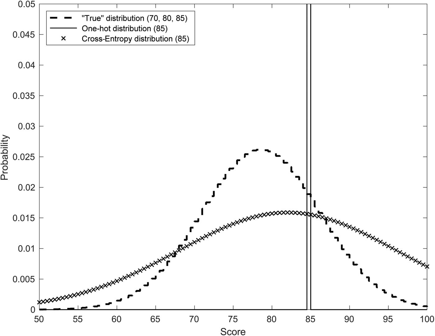
Figure 2. Three distributions for Stellenbosch judge #20 on a blind triplicate.
The difference between the “true” distribution and the one-hot distribution is error that can be quantified as cross-entropy. Likewise, the difference between the cross-entropy Equation (4) distribution and the “true” distribution is error that can again be quantified as cross-entropy. The cross-entropy errors for the example in Figure 2 are 20.0 and 4.3, respectively. Although not close to a perfect fit to the true distribution, the solution to Equation (4) is more accurate than using only an observed rating. The cross-entropy errors for all of the Stellenbosch triplicate observations appear in Figure 3. As a check, the sum of squared differences between the same pairs of distributions is also shown in Figure 3.
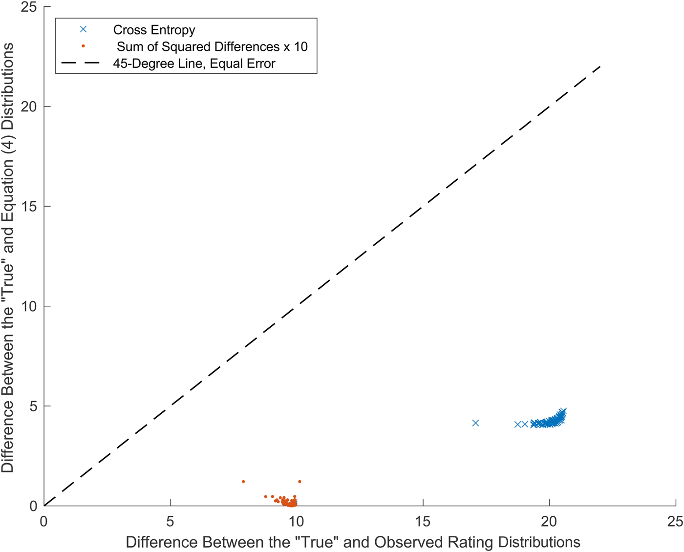
Figure 3. Errors in estimates of the “True” distributions for Stellenbosch blind triplicates (30 judges, 90 observations).
The striking result in Figure 3 is that error in estimating the “true” distribution is materially and consistently lower using the solution to Equation (4) than when using only an observed rating. Results cluster below the 45-degree line in Figure 3, along which errors for the two methods are equal. The average cross-entropy using Equation (4) is 4.2, the average using a rating observed is 20.0, and 4.2 / 20.0 = 21%. Similar results are obtained when error is measured using sums of squared differences and when using KL Divergence. The blindness to all uncertainty caused by using only an observed rating yields larger errors than the broadness of a maximum entropy solution. The Stellenbosch data and MATLAB code for Figures 2 and 3 are available upon request.
VII. Conclusion
Wine judges assess wines and assign ratings that are discrete and within bounded sets of scores, ordered categories, or ranks. But much evidence shows that, although they are not merely random, those assignments are both stochastic and heteroscedastic. Those assignments may also be affected by anchoring, expectations, and serial position biases. The distribution of a rating observed is then wine- and judge-specific. Estimating the distribution of a rating to support ratings-related research or to calculate consensus among judges is thus acutely difficult because the sample size drawn from a latent wine- and judge-specific distribution is usually one.
The parameters in a PMF expressing the latent distribution of a rating observed can be estimated using the simple maximum entropy estimator in Equation (4). That estimator incorporates the information from zero, one, a few blind replicates, or many observations, and it relies on a minimum of additional assumptions. An example yields results in Figure 1 that are consistent with the results of experiments in which blind replicates are embedded within flights of wines that are evaluated by trained and tested judges. An application to the published tasting data in Figures 2 and 3 shows that the maximum entropy estimator has, for the Stellenbosch triplicates, less than 25% of the error found using observed ratings alone.
An essential aspect of the maximum entropy solution to Equation (4) is that the solution is not an assertion that a judge's ratings have a nearly random distribution. But it is an assertion that evident knowledge about the distribution, based on a small sample, may support a distribution that is only a little better than random. That makes sense for an anonymous judge about whom nothing is known. If a researcher has information that a judge has perfect consistency, then the PMF for that judge is a one-hot vector. If a researcher has information that Jancis Robinson, James Suckling, or some other critic has very good consistency, then the PMF in Equation (4) for that critic can have a small dispersion. Whatever the capability of a judge, Equation (4) is both flexible and explicit.
Equation (4) is intended as a tool to support ratings-related research and assessments of consensus among judges. Research may lead to improvements in or application-specific variations of Equation (4). Adding terms to Equation (4) may enable analysis of anchoring, expectation, and other biases. Further tests of the estimator could include estimating parameters in PMFs from cross-section ratings data. On that foundation, the assumption that ratings are deterministic or IID, which is implicit in much current research and most calculations of multi-judge consensus, could be relaxed. Aggregates that depend on sums and research that uses ratings in transformations or regressions can be reframed using Equation (4), as maximum likelihood functions that are explicit about the uncertainty surrounding a rating observed.
Acknowledgments
The author thanks the Editor and reviewers for their perceptive and constructive comments on a draft.
Appendix A: Literature review regarding what can be deduced about the shape of a latent distribution from one observation
Rodriguez (Reference Rodriguez, Skilling and Sibisi1996) reports that, in 1964, Robert Machol derived a confidence interval (CI) for an estimate of the mean of an unbounded distribution that is symmetric about zero. Rodriguez re-stated Machol's result, presented an unpublished non-parametric CI for $\hat{\mu }$ that he attributed to Herbert Robbins, and derived a CI for the standard deviation ($\hat{\sigma }$
 ) of an unbounded symmetric distribution.
Golan, Judge, and Miller (Reference Golan, Judge and Miller1996, pp. 115–123) examined least squares, maximum likelihood, Bayesian and maximum entropy methods of estimating, for one observation, the mean of a bounded distribution that is symmetric about zero. Based on what those authors describe as “standard sampling theory,” the least squares and maximum likelihood methods yield $\hat{\mu } = x^o$ . Their results using Bayes Rule cite and match Casella and Strawderman (Reference Casella and Strawderman1981). Their maximum entropy estimate of $\hat{\mu }$
 is a Lagrange function of information entropy and an exogenous constraint on the difference between x o and the unobserved μ. Both the Bayesian and the maximum entropy solutions show that as the range of x increases, $\hat{\mu }$
 tends away from x o toward the center of the range. Golan, Judge, and Miller compare the accuracy of the four methods assuming several types of error distribution, and they conclude that the maximum entropy method both relies on the least restrictive assumptions and is the most accurate.
Leaf, Hui, and Lui (Reference Leaf, Hui and Lui2009) examined Bayesian estimates of distribution parameters using a single observation. The authors found that reasonable Bayesian results depend very much on starting with a reasonable prior, and they recommend further development of axiomatic or so-called fiducial inference. Primavera (Reference Primavera2011) addressed estimating the mean of a bounded distribution from one observation using a sample mean, maximum likelihood estimator, Bayesian inference, and game theory. The sample mean for one observation implies merely $\hat{\mu } = x^o$ . A maximum likelihood estimate yields the same result but interposes a distribution function, and Bayes’ Rule yields results, like those found by Leaf, Hui, and Lui, that depend on the prior and the form of the distribution function.
Cook and Harslett (Reference Cook and Harslett2015, pp. 11–22) used one observation and cross-entropy to estimate the intercept and slope of a linear equation. Following Bayes, they assumed prior probability distributions for the two parameters and then selected values for those parameters that minimized an exogenously-weighted cross-entropy subject to the Lagrange constraints that the probabilities sum to unity and that the linear function of the parameters yields x o.
Appendix B: Derivation of equation (4)
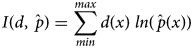
See definitions of algebra in Section IV and assume an arbitrary distribution (d).
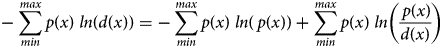
Some authors equate cross-entropy and Kullback-Leibler Divergence. See, for example, Shore and Johnson (Reference Shore and Johnson1981, p. 472) and Golan, Judge, and Miller (Reference Golan, Judge and Miller1996, p. 29) compared to Shannon (Reference Shannon1948, p. 14), Rioul (Reference Rioul2008, p. 61), and numerous machine learning references, including Mitchell (Reference Mitchell1997, p. 57). This article employs the definitions in Equation (B1) that are consistent with Shannon, Rioul, and machine learning references: Cross-Entropy = Entropy + KL Divergence.
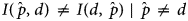
Equation (B2) expresses that H(d) is less than the maximal H(u). Entropy and cross-entropy are non-linear functions, and Equation (B3) expresses that cross-entropy is not a metric or symmetric unless $\hat{p} = d$ .
.

The distributions u and q|x 0 are known and fixed. For a known and fixed d, solving for parameters in a PMF $\hat{p}$ to obtain d implies minimizing the form $I( {d, \;\hat{p}} )$
 in Equations (B4) and (B5). See Shore and Johnson (Reference Shore and Johnson1981, pp. 472–473) and Golan, Judge, and Miller (Reference Golan, Judge and Miller1996, p. 41) on minimizing cross-entropy. As a check, examples in MATLAB code are available on request from the author.
The two conditions in Equations (B6) and (B7) must hold. The symbol for approximately equal (≈) indicates that the solution will be a minimum difference, but due to the form of a PMF, it may not be a precise equality (=).
Find $\hat{p}$ at the minimum difference between u and q|x 0 in Equation (B8). A transformation function using (1/(1 + n)) enforces the conditions in Equations (B6) and (B7). See an example of adding cross entropies in a transformation function using weights w and (1 – w) at Golan, Judge, and Miller (Reference Golan, Judge and Miller1996, p. 111). Other transformations that could be considered include multiplier, exponential, inverse variance, and entropy-related functions.Footnote 16 Again, examples in MATLAB code are available on request from the author.


 Open access