


Introduction
One of the central questions in ecology is what controls the distribution of species. This question has become more urgent because climate change is forcing species to track suitable climatic conditions and shift their distribution ranges either poleward or upward (Chen et al. Reference Chen, Hill, Ohlemüller, Roy and Thomas2011, IPCC Reference Field, Barros, Dokken, Mach, Mastrandrea, Bilir, Chatterjee, Ebi, Estrada, Genova, Girma, Kissel, Levy, MacCracken, Mastrandrea and White2014). Particularly in montane landscapes in (sub-)tropical biomes, the presence of steep mountain ranges and shallow latitudinal gradient in climatic conditions is likely to leave plant species with only one option – shifting their ranges upward. In these landscapes, such shift in species distribution ranges will be particularly problematic for plant species with narrow elevational ranges as they are likely to be forced to move upward rapidly to maintain viable population sizes, and for those living near mountain tops as smaller land surface area is available at higher elevations (Körner Reference Körner2007). To better understand the fate of montane plant species in the face of climate change, it is urgently needed to understand which environmental factors best predict their distribution and how they are spatially distributed in montane landscapes.
The elevational gradient (sometimes referred to as an ‘altitudinal gradient’) is an ideal system to study the multiple factors that control species distribution, as it presents a complex, multiple-factor gradient that affects plant species distribution in multiple ways. Temperature, solar radiation, precipitation and soil properties are important determinants of plant species distribution, since they set the local site conditions and thus the abiotic niches (Hemp Reference Hemp2006). Temperature decreases linearly with increasing elevation, and it regulates plant metabolic rates that are vital for plant survival, growth and reproduction. Lower temperature at higher elevations may not only impair plant performance but also lead to slower soil microbial activity and other soil processes, hence lower nutrient availability (Müller et al. Reference Müller, Schickhoff, Scholten, Drollinger, Böhner and Chaudhary2016a, Vincent et al. Reference Vincent, Sundqvist, Wardle and Giesler2014). Under clear sky, solar radiation increases with increasing elevation because of reduced atmospheric turbidity. But the amount of solar radiation received by organisms depends on clouds and fog, and both often increase with increasing elevation (Adhikary Reference Adhikary2012, Körner Reference Körner2007). Consequently, in the areas often covered with clouds, productivity of montane species may be strongly limited by irradiance (Fyllas et al. Reference Fyllas, Bentley, Shenkin, Asner, Atkin, Díaz, Enquist, Farfan-Rios, Gloor, Guerrieri, Huasco, Ishida, Martin, Meir, Phillips, Salinas, Silman, Weerasinghe, Zaragoza-Castells and Malhi2017). With increasing elevation, in the subtropics, precipitation usually increases up to cloud condensation elevation and decreases beyond (Körner Reference Körner2007). Montane soils are, in general, poorly developed, stony, shallow, relatively infertile and often acidic. With increasing elevation, soils become thinner, less developed and less fertile (FAO 2015). Precipitation, evapotranspiration, topography and soil water-holding capacity determine water availability, hence plant survival. Particularly in steep montane landscapes, thin, stony and infertile soils have a low water-holding capacity, which impedes seedling and sapling establishment (Müller et al. Reference Müller, Schickhoff, Scholten, Drollinger, Böhner and Chaudhary2016a, Reference Müller, Schwab, Schickhoff, Böhner and Scholten2016b). Additionally, diurnal and seasonal variability of environmental factors increase with increasing elevation (Rasmann et al. Reference Rasmann, Alvarez and Pellissier2014) exposing high elevation plants to comparatively harsher, more stressful and variable environmental conditions. All the aforementioned environmental factors play crucial roles in shaping plant species distribution along elevational gradients; however, their relative importance is still contested (Bhattarai et al. Reference Bhattarai, Vetaas and Grytnes2004, Dubuis et al. Reference Dubuis, Giovanettina, Pellissier, Pottier, Vittoz and Guisan2013, Müller et al. Reference Müller, Schickhoff, Scholten, Drollinger, Böhner and Chaudhary2016a).
Rapoport’s elevational rule
The elevational ranges of various groups of organisms (trees, mammals, birds, reptiles, insects and amphibians) increase with increasing elevation, a phenomenon which has been coined ‘Rapoport’s elevational rule’ (Stevens Reference Stevens1992). Stevens (Reference Stevens1992) suggested that these wider ranges are the result of higher climatic variability that species experience at higher elevations. The climatic variability hypothesis (more generally the environmental variability hypothesis) posits that species occurring in climatically variable habitats, such as those at high elevations, would develop wider environmental tolerances and, hence, occupy wider elevational ranges than species occurring in climatically stable habitats, such as those at low elevations (Pintor et al. Reference Pintor, Schwarzkopf and Krockenberger2015, Stevens Reference Stevens1992). The generality of Rapoport’s elevational rule is still contested – some studies found strong support for it (Pintor et al. Reference Pintor, Schwarzkopf and Krockenberger2015, Rasmann et al. Reference Rasmann, Alvarez and Pellissier2014, Schellenberger Costa et al. Reference Schellenberger Costa, Gerschlauer, Kiese, Fischer, Kleyer and Hemp2018, Subedi et al. Reference Subedi, Bhattarai, Perez and Sah2020), while others have found little (Feng et al. Reference Feng, Hu, Wang and Wang2016) or no support (Bhattarai & Vetaas Reference Bhattarai and Vetaas2006, Lee et al. Reference Lee, Chun, Song and Cho2013, Vetaas & Grytnes Reference Vetaas and Grytnes2002).
In this study, we focused on the Himalayan elevation gradient in Nepal because 1) it is one of the longest and steepest elevational gradients in the world, 2) it is a global hotspot of biodiversity (Mittermeier et al. Reference Mittermeier, Robles Gil, Hoffmann, Pilgrim, Brooks, Mittermeier, Lamoreux and Da Fonsec2004), 3) global warming is forcing numerous treeline species along this gradient to move upward at a rate as high as 26 m per decade (Chhetri et al. Reference Chhetri, Gaddis and Cairns2018, Gaire et al. Reference Gaire, Koirala, Bhuju and Borgaonkar2014, Suwal et al. Reference Suwal, Shrestha, Guragain, Shakya, Shrestha, Bhuju and Vetaas2016), and 4) the distribution of species along an elevational gradient according to Rapoport’s elevational rule can be tested along this gradient. Some studies have reported unimodal patterns in tree species elevational ranges along this elevational gradient (Bhattarai & Vetaas Reference Bhattarai and Vetaas2006, Vetaas & Grytnes Reference Vetaas and Grytnes2002), while others have reported a monotonic increase in elevational ranges among other groups of plant species (Feng et al. Reference Feng, Hu, Wang and Wang2016, Subedi et al. Reference Subedi, Bhattarai, Perez and Sah2020) supporting Rapoport’s elevational rule. These studies used an elevation band (100 m bands) approach. Firstly, based on the data on species elevational ranges in the published floral databases, they estimated species elevational ranges as the differences between the maximum and minimum elevations of species rounded to the nearest 100 m and elevational midpoints as the averages of the elevational limits of species. Then, they used average elevational ranges of all species that occur in each elevation band or species whose elevational midpoints occur in each elevation band to evaluate the relationship between species elevational ranges and elevation. However, species elevational midpoints and average elevational ranges based on presence records may not be representative of the species’ elevational optima – points where species occurrence or abundance peak (Pintor et al. Reference Pintor, Schwarzkopf and Krockenberger2015), and elevational tolerance – the elevational range where species could actually occur. For example, the elevational midpoint of a species with its elevational ranges between 100 and 1500 m a.s.l. is 800 m a.s.l. However, its elevational optimum may be higher or lower than 800 m a.s.l. depending on whether species abundance is left- or right-skewed. The species’ elevational optima should be in the middle of species’ niches rather than the middle of their elevational ranges, and the modelled ecological niches and their projected spatial distributions may provide a better measure of species’ elevational tolerance than the elevation of presence records alone. Therefore, in this study, we used MaxEnt (Phillips et al. Reference Phillips, Dudík and Schapire2004, Reference Phillips, Anderson and Schapire2006) to model ecological niches and project spatial distributions of 277 plant species that are most common among the 1169 inventoried plant species and that belong to 9 different life forms and subsequently used these niches and distribution maps to calculate species’ elevational optima and ranges (see Methods for details).
Here we addressed two research questions. First, which environmental factors best predict the distribution of plant species along an elevational gradient? We hypothesized that temperature would be the key environmental factor that best predicts the distribution of plant species along an elevational gradient because it 1) decreases predictably with elevation, 2) directly influences plant physiology and soil processes vital for plant survival, growth and reproduction, and 3) constrains growth of plant species by controlling growing season length. Second, how do species’ elevational ranges change with elevation along an elevational gradient? We hypothesized that plant species living at high elevations, where environmental conditions are harsher, more stressful and variable, would have wider physiological tolerances to environmental conditions and occupy broader elevational ranges compared to plant species living at low elevations, where environmental conditions are more benign and stable, according to Rapoport’s elevational rule (Pintor et al. Reference Pintor, Schwarzkopf and Krockenberger2015, Stevens Reference Stevens1992).
Methods
Study site
For our study, we selected the Himalayan elevational gradient in Nepal, one of the longest and steepest elevational gradients in the world. Within a horizontal span of mere 200 km, elevation varies from 60 m a.s.l. in the south to the highest peak of the world in the north (HMGN/MFSC 2002) resulting in a roughly south-facing elevational gradient. Along the gradient, trees can grow at up to 4000 m a.s.l. (treeline) while alpine meadows can be found at up to 5000 m a.s.l. (TISC 2002). Temperature decreases linearly along this gradient (Lillesø et al. Reference Lillesø, Shrestha, Dhakal, Nayaju and Shrestha2005), and precipitation shows a mid-elevation maximum (Acharya et al. Reference Acharya, Vetaas and Birks2011, Kansakar et al. Reference Kansakar, Hannah, Gerrard and Rees2004). This gives rise to an extensive bioclimatic gradient ranging from wet, warm and stable tropical climate in the lowlands in south to cold, more stressful and variable alpine climate in the Himalayas in the north (HMGN/MFSC 2002, Lillesø et al. Reference Lillesø, Shrestha, Dhakal, Nayaju and Shrestha2005). As a result of this elevation-driven variation in environmental conditions and habitats, Nepal is a home to disproportionately higher percentage of the world’s flora and fauna (5.1% of gymnosperms, 2.7% of angiosperms, 9.3% of birds and 4.5% of mammals in 0.1% of global land area, HMGN/MFSC 2002) – a global hotspot of biodiversity (Mittermeier et al. Reference Mittermeier, Robles Gil, Hoffmann, Pilgrim, Brooks, Mittermeier, Lamoreux and Da Fonsec2004).
MaxEnt
As modelled ecological niches and their projected spatial distributions may provide a better measure of species’ elevational tolerance than the elevation of presence records alone, we used a modelling approach. MaxEnt version 3.3.3k (Phillips et al. Reference Phillips, Dudík and Schapire2004, Reference Phillips, Anderson and Schapire2006) was selected over other species distribution modelling (SDM) algorithms because 1) it is a powerful presence-only SDM algorithm that can efficiently handle complex interactions between species presence records and environmental predictors (Elith et al. Reference Elith, Graham, Anderson, Dudík, Ferrier, Guisan, Hijmans, Huettmann, Leathwick, Lehmann, Li, Lohmann, Loiselle, Manion, Moritz, Nakamura, Nakazawa, Overton, Peterson, Phillips, Richardson, Scachetti-Pereira, Schapire, Soberón, Williams, Wisz and Zimmermann2006, Reference Elith, Phillips, Hastie, Dudík, Chee and Yates2011), 2) it makes relatively accurate predictions with small number of presence records (Pearson et al. Reference Pearson, Raxworthy, Nakamura and Peterson2007, van Proosdij et al. Reference Van Proosdij, Sosef, Wieringa and Raes2016, Wisz et al. Reference Wisz, Hijmans, Li, Peterson, Graham and Guisan2008), 3) it has been reported to outperform other SDM algorithms (Aguirre-Gutiérrez et al. Reference Aguirre-Gutiérrez, Carvalheiro, Polce, Van Loon, Raes, Reemer and Biesmeijer2013, Elith et al. Reference Elith, Graham, Anderson, Dudík, Ferrier, Guisan, Hijmans, Huettmann, Leathwick, Lehmann, Li, Lohmann, Loiselle, Manion, Moritz, Nakamura, Nakazawa, Overton, Peterson, Phillips, Richardson, Scachetti-Pereira, Schapire, Soberón, Williams, Wisz and Zimmermann2006, Giovanelli et al. Reference Giovanelli, De Siqueira, Haddad and Alexandrino2010, Hao et al. Reference Hao, Elith, Lahoz-Monfort and Guillera-Arroita2020, Merckx et al. Reference Merckx, Steyaert, Vanreusel, Vincx and Vanaverbeke2011, Wisz et al. Reference Wisz, Hijmans, Li, Peterson, Graham and Guisan2008), 4) it does not require species absence records which are difficult to confirm (MacKenzie Reference MacKenzie2005, Raes & Aguirre-Gutiérrez Reference Raes, Aguirre-Gutiérrez, Hoorn, Perrigo and Antonelli2018), and 5) it allows using all species presence records available in floral databases and natural history collections. For their improved predictive performances, ensemble models are increasingly being used for SDM (Aguirre-Gutiérrez et al. Reference Aguirre-Gutiérrez, Carvalheiro, Polce, Van Loon, Raes, Reemer and Biesmeijer2013, Araújo & New Reference Araújo and New2007, Hao et al. Reference Hao, Elith, Lahoz-Monfort and Guillera-Arroita2020). However, it is very difficult to estimate contributions of individual environmental variables to the final species distribution model from an ensemble model. As one of our main aims is to identify key environmental factors that best predict plant species distribution along the elevational gradient (factors contributing the most to species distribution models), MaxEnt alone was used instead of ensemble of different SDM algorithms. MaxEnt uses species presence records, environmental predictors and randomly drawn background samples to model species’ ecological niches and project their spatial distributions.
Study species and their presence records
The national forest inventory (2010–2014) undertaken by Forest Research and Training Centre (then Department of Forest Research and Survey) Nepal served as the main source of species presence records. Two-phase stratified systematic cluster sampling was used for the inventory. In the first phase, Nepal was divided into 4 × 4 km grids. At each grid node, a sample cluster of 4–6 concentric circular plots (four (2 × 2) plots 300 m apart in north-south and east-west directions in lowlands with relatively homogenous forests, and six (3 × 2) plots 150 m apart in north-south and 300 m apart in east-west directions in hills and mountains with heterogeneous forests) was positioned starting at the grid node and moving first towards north and then towards east. Each plot had four concentric circular subplots of radii 4, 8, 15 and 20 m that were used to identify the trees to species and measure individual stem diameter at breast height (DBH), and tree height of trees of DBH ranges 5–9.9, 10–19.9, 20–29.9 and 30 cm and more, respectively. In addition to that each plot had four 1 m2 subplots each located 5 m away from the centre of the plot in four cardinal directions that were used to assess species-wise stem count of non-woody vascular plants. Next, each plot had four circular subplots of 2 m radii each located 10 m away from the centre of the plot in four cardinal directions that were used to assess species-wise stem count and mean height of seedlings, saplings and shrubs with DBH <5 cm. In the second phase, 450 sample clusters representing 2544 sample plots located in the forests below 4000 m a.s.l. and with a slope <45° were selected for field measurements (for details see DFRS 2015). Of these 2544 sample plots, we used species presence data from 2039 sample plots for which plant species were reliably identified to species level. Plant species names were standardized using multiple sources (Tropicos, Taxonomic Name Resolution Service, The Plant List and The International Plant Names Index) and, in case of discrepancies, verified by a taxonomist from Tribhuvan University, Nepal, to synonymize all taxonomic names to their currently accepted taxonomic names. In case of conflict, the currently accepted taxonomic names in The Plant List were used. Finally, of the 1169 inventoried plant species, 333 species (167 tree, 85 shrub, 31 herb, 14 fern, 14 grass, 14 liana, 5 orchid, 2 palm and 1 sedge species) were recorded in at least 10 unique sample plots and were selected for the study. The detailed list of the selected plant species is presented in Supplementary Table 1. Orchid was used as a separate life form to be consistent with the national forest inventory, Nepal database – that was used as the main source of species presence records for this study.
To supplement the aforementioned surveyed presence records, additional presence records were compiled from the online floral databases (Global Biodiversity Information Facility: http://www.gbif.org, Integrated Digitized Biocollections: http://www.idigbio.org and iNaturalist: http://www.inaturalist.org) and supplementary fieldwork (undertaken in Oct–Dec 2017). Both currently accepted taxonomic names and their unambiguous synonyms retrieved from The Plant List – that was used as the starting point for the taxonomic backbone of the World Flora Online – were used to download presence records from the online floral databases. Citations for the records thus downloaded are presented in Supplementary Table 4.
Cleaning species presence records
The species presence records were cleaned in two steps. In the first step, all duplicate records (using currently accepted taxonomic names and their synonyms to download records from the online floral databases returned duplicate records); records based on fossil specimens, and plants not from wild; records with missing coordinates, zero coordinates, coordinates with latitude = longitude (impossible in case of Nepal), invalid coordinates, and coordinates likely to be based on country centroids or country capitals (records within threshold of 0.0083 degrees ≈ 1 km of country centroids or country capitals); records with coordinates country mismatch; and records with coordinates uncertainty ≥1 km were removed using process described in the R package speciesgeocodeR (Zizka & Antonelli Reference Zizka and Antonelli2015). To avoid pseudo-replication, all duplicates at 0.0083 degrees ≈ 1 km spatial resolution (also the raster resolution of environmental predictors, see below) were also removed.
In the second step, species’ elevational ranges reported in published literature (Fraser-Jenkins et al. Reference Fraser-Jenkins, Kandel and Pariyar2015, Fraser-Jenkins & Kandel Reference Fraser-Jenkins and Kandel2019, http://www.efloras.org/ 2019, Jackson Reference Jackson1994, Paudyal & Haq Reference Paudyal and Haq2008, Rajbhandari & Rai Reference Rajbhandari and Rai2019, Shrestha et al. Reference Shrestha, Bhattarai and Bhandari2018) were used to identify and discard doubtful presence records, that is presence records beyond the reported species’ elevational ranges. Furthermore, to make sure the cleaned presence records are representative of the reported species’ elevational ranges, species with presence records covering <50% of the reported elevational ranges were also discarded. This reduced the number of spatially unique presence records to 10 775 and the number of selected plant species to 281 with per species spatially unique presence records ranging from 3-324. Since cleaning of species presence records reduced the number of spatially unique presence records of four out of 281 species to less than five, that is the absolute minimum number of presence records required for MaxEnt modelling (Pearson et al. Reference Pearson, Raxworthy, Nakamura and Peterson2007, van Proosdij et al. Reference Van Proosdij, Sosef, Wieringa and Raes2016), only 277 species (143 tree, 76 shrub, 23 herb, 13 grass, 9 liana, 7 fern, 4 orchid, 1 palm and 1 sedge species) were considered for further analysis.
Environmental predictors
To avoid edge effects as result of modelling truncated niches (Raes Reference Raes2012), we defined Nepal plus 200 km buffer surrounding the Nepalese border as our area of interest. We included this buffer to include a wide range of environmental conditions, so that it is easier to model the drivers of species distribution. To relate species presence records to environmental predictors, 53 climatic, topographic and edaphic variables were compiled. Freely available global datasets were downloaded, cropped to the area of interest, and aggregated to 30 arc-seconds (∼1 km) spatial resolution, as and when necessary. Climatic variables (monthly temperature, precipitation, solar radiation, wind speed and water vapour pressure, and 19 bioclimatic variables) were downloaded from WorldClim (http://worldclim.org/version2, Fick & Hijmans Reference Fick and Hijmans2017). WorldClim 2 was selected because it has improved estimates for areas with low station density and areas with sharp gradients such as rain-shadows (Fick & Hijmans Reference Fick and Hijmans2017). Mean annual solar radiation, wind speed and water vapour pressure were computed using WorldClim 2 monthly data. Aridity (Thornthwaite’s aridity index), climatic moisture index, growing degree days (base temperature = 10 ˚C) and potential evapotranspiration (annual PET, PET extremes and PET seasonality) were computed using WorldClim 2 monthly data using ENVIREM R package (Title & Bemmels Reference Title and Bemmels2018). Cloud cover variables (mean annual cloud frequency and cloud cover seasonality) were downloaded from EarthEnv (http://www.earthenv.org/cloud, Wilson & Jetz Reference Wilson and Jetz2016). Maximum climatic water deficit (MCWD) was computed using WorldClim 2 monthly data based on Malhi et al. Reference Malhi, Aragao, Galbraith, Huntingford, Fisher, Zelazowski, Sitch, McSweeney and Meir2009.
Soil variables were downloaded from ISRIC-SoilGrids (ftp://ftp.soilgrids.org/data/aggregated/1km/, Hengl et al. Reference Hengl, De Jesus, Heuvelink, Gonzalez, Kilibarda, Blagotić, Shangguan, Wright, Geng, Bauer-Marschallinger, Guevara, Vargas, MacMillan, Batjes, Leenaars, Ribeiro, Wheeler, Mantel and Kempen2017). SoilGrids provides predictions at seven standard depths (0, 5, 15, 30, 60, 100 and 200 cm) for standard soil variables like organic carbon, bulk density, cation exchange capacity (CEC), pH, soil texture fractions, coarse fragments, available water capacity and water content. As topsoil conditions determine whether a seedling can establish or not, the first four SoilGrids layers were used to compute the weighted average over a depth interval of 0–30 cm, that is topsoil, using trapezoidal rule for numerical integration (Hengl et al. Reference Hengl, De Jesus, Heuvelink, Gonzalez, Kilibarda, Blagotić, Shangguan, Wright, Geng, Bauer-Marschallinger, Guevara, Vargas, MacMillan, Batjes, Leenaars, Ribeiro, Wheeler, Mantel and Kempen2017).
Topographic variables like elevation, aspect and slope were computed using digital elevation model downloaded from CGIAR-CSI (https://cgiarcsi.community/data/srtm-90m-digital-elevation-database-v4-1/). Finally, distance to water sources was computed using river network data downloaded from HydroSHEDS (http://www.hydrosheds.org/) and global lakes and wetlands data downloaded from WWF (https://www.worldwildlife.org/pages/global-lakes-and-wetlands-database). The detailed list of thus compiled 53 environmental variables is presented in Supplementary Table 2.
Selection of environmental predictors for MaxEnt modelling
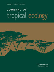
As multicollinearity among environmental variables can distort model estimation and prediction, we used a Spearman’s rank correlation coefficient of 0.7 as threshold to identify highly correlated environmental variables (Dormann et al. Reference Dormann, Elith, Bacher, Buchmann, Carl, Carr, Garc, Gruber, Lafourcade, Leit, Tamara, Mcclean, Osborne, Der, Skidmore, Zurell and Lautenbach2013). Correlations among environmental variables are presented as a cluster dendrogram and as a bivariate correlation matrix in Figure 1 and Supplementary Table 3, respectively. Then, to identify the variables that best describe the ecological variations along the studied elevational gradient, we used a principal component analysis (PCA). Loadings of environmental variables along the first two principal components are presented in Supplementary Figure 1. As we were interested in modelling elevational distributions of species based on their observed presence records, we used 52 environmental variables (elevation excluded) of 1437 spatially unique presence locations (of 281 species left after cleaning) for correlation analysis and PCA. Also, the results were similar when doing correlation analysis and PCA on the whole area of interest (data not shown). Highly correlated environmental variables are not necessarily ecologically redundant, but they often have the same spatial patterns and cannot always be distinguished. Therefore, from each cluster of highly correlated variables, we selected one variable that was thought to be the ecologically most relevant factor that determines the elevational distribution of species and/or that had highest loading along one of the first three principal components. This resulted in a selection of 19 least correlated environmental variables (10 climatic, 6 edaphic and 3 topographic, Table 1). To represent the cluster of correlated temperature (e.g. temperature extremes) and non-temperature variables (such as irradiance and PET), we selected mean annual temperature (MAT). Although temperature extremes (e.g. maximum temperature of warmest month, minimum temperature of coldest month) may co-shape species distribution boundaries, we believe that MAT is more important in shaping species performance and distribution. Across the 1437 spatially unique presence locations, MAT is closely correlated with maximum temperature of warmest month (Spearman’s rank r = 0.99, p < 0.001) and with minimum temperature of coldest month (Spearman’s rank r = 0.98, p < 0.001). Hence, to avoid multicollinearity problems we used only MAT, as it captures both the variation in summer and winter temperature, and the average growing conditions during the year.
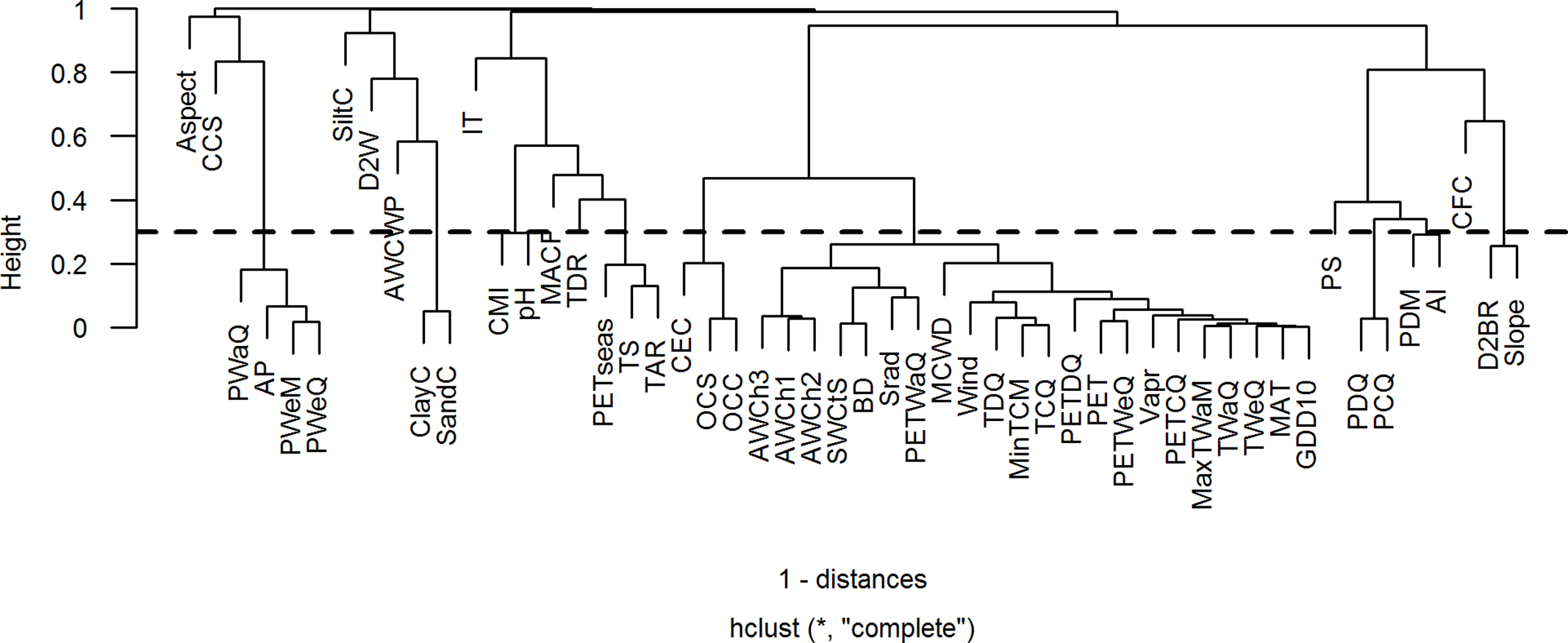
Figure 1. Cluster dendrogram showing correlation among environmental variables. Fifty-two environmental variables (elevation excluded) of 1437 spatially unique presence locations were used for the correlation analysis. In this case, a height of 0.3, indicated by dotted line, is taken as a threshold. Height is defined as 1 – Spearman’s rank correlation coefficient. All the variables with height ≤ 0.3 (or Spearman’s rank correlation coefficient ≥ 0.7) are considered highly correlated. Details of environmental variable abbreviations used in the plot are presented in Supplementary Table 2.
Table 1. List of 19 least correlated environmental variables selected for this study. Variable categories, sub-categories, names and their corresponding units and abbreviations are shown.

MaxEnt modelling
Samples with data (SWD) format of MaxEnt version 3.3.3k (Phillips Reference Phillips2010) in R package dismo (Hijmans et al. Reference Hijmans, Phillips, Leathwick and Elith2017) were used to construct species distribution models for 277 plant species. As we were interested in modelling elevational distributions of species based on their observed presence records, we used 1437 spatially unique presence locations as background sample. To comply with the ecological theory that species responses to environmental gradients are often unimodal (Austin Reference Austin2007), MaxEnt was restricted to use only linear and quadratic features (Boucher-Lalonde et al. Reference Boucher-Lalonde, Morin and Currie2012, Merow et al. Reference Merow, Smith and Silander2013), where linear features represent one side of a unimodal response due to partial representation of the entire gradient.
To test the significance of the models, we compared the AUC (area under the receiver operating characteristic curve) values of the models to the AUC values of the bias-corrected null models, that is models based on the random presence records (Raes & Ter Steege Reference Raes and Ter Steege2007). For this, for each species, 100 bias-corrected null models were constructed with the presence records randomly drawn from 1437 spatially unique presence records. The number of randomly drawn presence records was kept equal to the number of true presence records of the target species. The models with AUC values >95th percentile AUC value of the null models were considered to perform significantly better than expected by chance. Only the significant models were retained for further analysis.
Data analysis
To evaluate which environmental factors best predict the distribution of plant species along an elevational gradient, we analysed the frequency with which environmental variables were found to be the most important (cf. Bradie & Leung Reference Bradie and Leung2016). For this, for each species with a significant species distribution model, we identified the environmental variable that contributed the most to the model (i.e. the most important environmental variable) based on the relative percentage contributions of the variables to the model.
To test whether species elevational ranges increase with increasing elevation along an elevational gradient, a simple linear regression was carried out with species’ elevational ranges and elevational optima. For this, firstly, all significant species distribution models were projected onto the geographical space using MaxEnt’s ‘density.Project’ function to derive probability of occurrence maps for the entire study area. Secondly, these maps were reclassified using ‘10 percentile training presence logistic threshold’ (one of the most conservative and absence independent thresholds in MaxEnt) to produce discrete presence-absence maps, that is species distribution maps (Liu et al. Reference Liu, White and Newell2011). Finally, these species distribution maps were used to compute species’ elevational distribution parameters, that is the elevational minimum, maximum, optimum and range. To have a conservative estimate of a species’ elevational distribution parameters, the 5th and 95th percentile elevation values were used as estimates of the elevational ‘minimum’ and ‘maximum’, respectively. The difference between elevational maximum and minimum was used as an estimate of the elevational ‘range’. The mid-value of the elevation class with the highest proportion of pixels predicted to be occupied was used as an estimate of the elevational ‘optimum’. For this, the distribution map of each species was classed into 100 m elevational bins, and for each elevational bin, the proportion of pixels predicted to be occupied was calculated. This procedure effectively corrects for the smaller available surface area at higher elevational bins. All calculations and analyses were done with R-3.4.3 (R Core Team 2017).
Limitations of methods
A few methodological limitations might have influenced our results. First, we used global environmental datasets with a spatial resolution of 1 × 1 km as sources of our environmental predictors. It is likely that these datasets did not fully capture all the local details in the Himalayas because i) the environmental conditions may vary over short distances in the Himalayas, and ii) the observed data that are bases of these global interpolations are sparse in the Himalayas (Deblauwe et al. Reference Deblauwe, Droissart, Bose, Sonké, Blach-Overgaard, Svenning, Wieringa, Ramesh, Stévart and Couvreur2016). However, in absence of reliable national/regional datasets these were the best datasets available for the study area.
Second, although it is established that species distributions are jointly regulated by abiotic environments and biotic interactions (e.g. Godsoe et al. Reference Godsoe, Franklin and Blanchet2017, MacArthur Reference MacArthur1972, Peterson et al. Reference Peterson, Soberón, Pearson, Anderson, Martínez-Meyer, Nakamura and Araújo2011, Soberón & Peterson Reference Soberón and Peterson2005, Wisz et al. Reference Wisz, Pottier, Kissling, Pellissier, Lenoir, Damgaard, Dormann, Forchhammer, Grytnes, Guisan, Heikkinen, Høye, Kühn, Luoto, Maiorano, Nilsson, Normand, Öckinger, Schmidt, Termansen, Timmermann, Wardle, Aastrup and Svenning2013), we did not account for biotic interactions as predictor variables in our study because biotic interactions are inherently complex, and especially so when we consider several species at a time. Moreover, although changes in land use may affect species distributions, we only focused here on natural forest vegetation and did not include land use change in the analysis. For example, in Nepal, nearly two-thirds of the total forest area is affected by grazing by free roaming cattle (DFRS 2015). Because standardized country-wide data on the occurrence and intensity of grazing are not available, we only focused on how climatic, edaphic and topographic environmental variables affect species distribution ranges.
Results
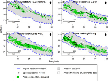
Out of 277 species, 255 species (92%) had distribution models performing significantly better than expected by chance. Only the significant models were retained for further analysis. Examples of the predicted species distribution maps are shown in Figure 2.
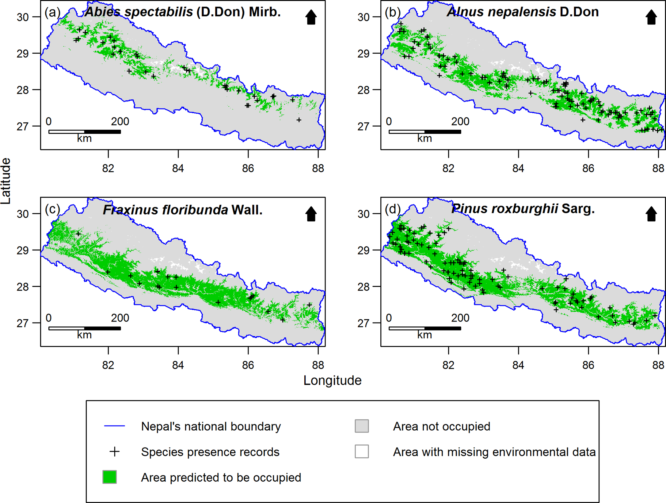
Figure 2. Examples of species distribution maps for four plant species as predicted by MaxEnt: a) Abies spectabilis, b) Alnus nepalensis, c) Fraxinus floribunda and d) Pinus roxburghii. Maps are clipped to Nepal. The blue line indicates national boundary of Nepal. The Government of Nepal published on 20th May 2020 a new political map including Kalapani, Lipulekh and Limpiyadhura inside the Nepal borders. As our research started in 2016, in our research, we used the previous version of map without these territories. Species presence records outside the green distribution areas represent the 10% of the presence records with the lowest MaxEnt probability of occurrence values used to threshold the distribution maps. Areas with missing environmental data were excluded from MaxEnt modelling.
Environmental factors predicting the distribution of plant species along the elevational gradient
All 255 species had a relationship with one or more of the environmental predictors. Mean annual temperature followed by soil clay content (ClayC) and slope were the most important environmental variables predicting the distribution of plant species along the elevational gradient. MAT contributed the most to the distributions of 139 out of 255 species (54.5%), followed by ClayC (10.2%) and slope (9.4%) (Figure 3). Examples of species’ response to MAT, ClayC and slope are shown in Figure 4. Spatial GIS maps of these three environmental variables are presented in Supplementary Figure 2.
Figure 3. Relative frequencies of environmental variables that had the highest contribution to the significant distribution models of 255 Himalayan plant species. The three most important variables were mean annual temperature (MAT), soil clay content (ClayC) and slope. For abbreviations of the other environmental variables, see Table 1.

Figure 4. Examples of probabilities of species occurrence as predicted by MaxEnt in relation to a) mean annual temperature (MAT, top panels), b) soil clay content (ClayC, middle panels) and c) slope (bottom panels). Each point represents one of the 906 794 1 × 1 km grids of the study area.
Relationship between elevational ranges and elevation along the elevational gradient
The species elevational ranges initially increased with the elevational optima of the species, but this increase peaked between 2000 and 3000 m a.s.l. and then decreased beyond 3000 m a.s.l. (Figure 5, adj.r 2 = 0.47, p < 0.001). Also, the results were similar when regression analysis was carried out with species elevational ranges and elevational midpoints (the averages of the lowest and highest elevations of species; data not shown). The majority of species had their elevational optima at or towards the lower end of the elevational gradient. There were comparatively more tree species at low elevations and more shrub species at high elevations. Liana species occurred mainly in the lowlands. As some of the life forms, for example fern, orchid and sedge had too few species for the comparison, we pooled them into a non-woody class together with herbs and grasses for this analysis. Some species showed wide distribution ranges irrespective of their elevational optima, for example Stephania japonica var. discolor (Blume) Forman and Cotoneaster ellipticus (Lindl.) Loudon (Figure 5).
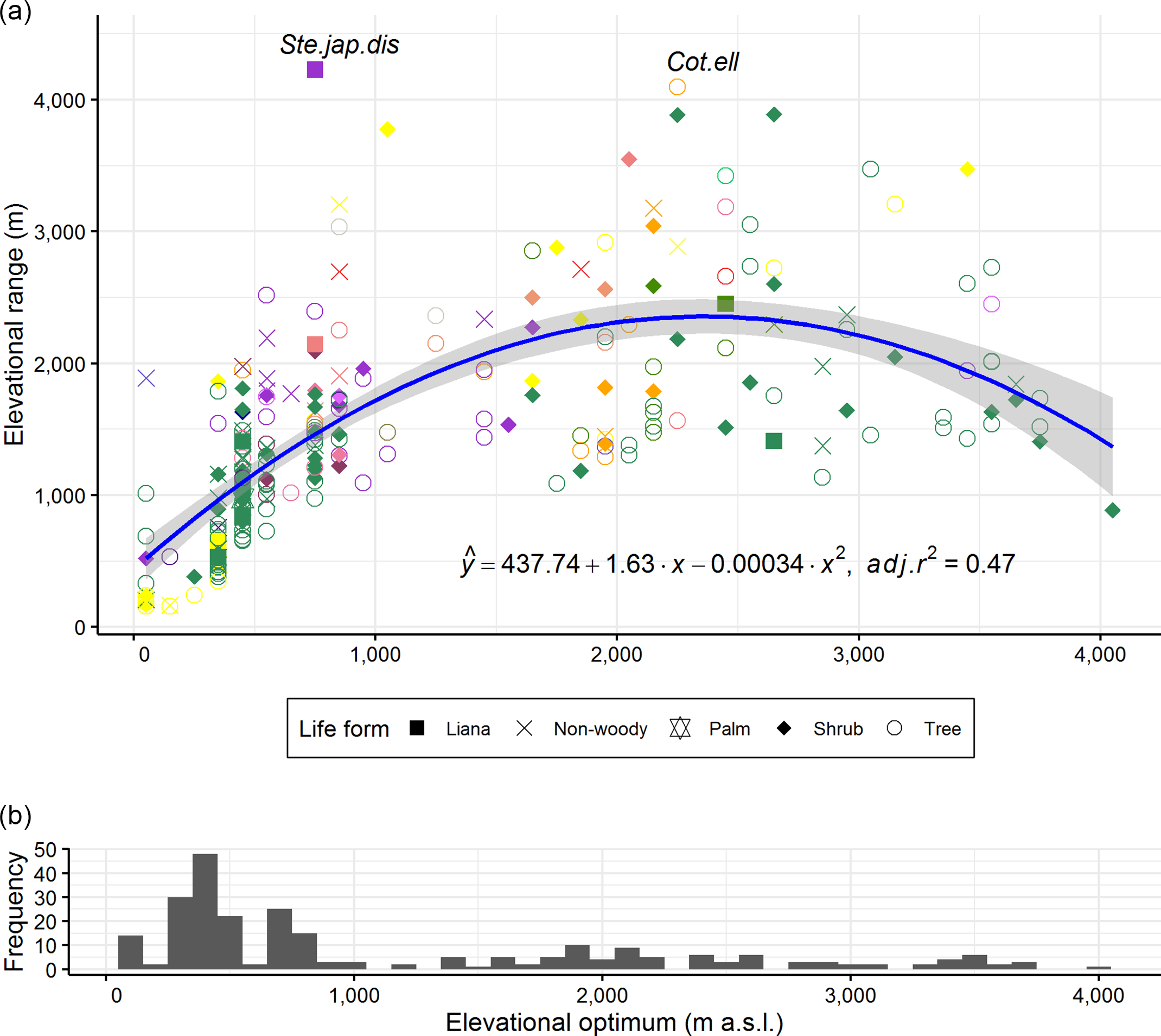
Figure 5. Relationship between elevational range and elevational optimum for 255 Himalayan plant species (represented by coloured shapes). Shapes correspond to life forms of the studied species. Ferns, grasses, herbs, orchids and sedges were grouped into a single non-woody class. Colours of shapes correspond to colours of environmental variables contributing the most to the models in Figure 3. Regression line and coefficient of determination (adj.r 2 ) are shown. Shade around regression line indicates 95% confidence interval. Both intercept and slopes are significant at p < 0.001. Adj.r 2 went up to 0.49 without outliers, that is without species labelled with their name abbreviations. Species name abbreviations used in the plot refer to first three letters of their genus, species and variety. The species list is shown in Supplementary Table 1. Histogram bars in the bottom panel are frequencies of species elevational optima along the gradient.
Discussion
We evaluated which environmental factors predict the distribution of plant species along an elevational gradient, and whether species’ elevational ranges increase with increasing elevation. We found that MAT followed by ClayC and slope are the key environmental factors predicting the distribution of plant species along an elevational gradient. Species elevational ranges showed a unimodal relationship with elevation.
It should be acknowledged that the importance of environmental factors may change with varying spatial scales of analysis (Blundo et al. Reference Blundo, Malizia, Blake and Brown2012). For example, we used environmental datasets with a spatial resolution of 1 × 1 km, which may conceal more subtle responses to local topography and elevational gradients. However, since our studied elevational gradient is very large (60 m a.s.l. in the south to 8848 m a.s.l. in the north), we think this is less of a problem. It should also be acknowledged that we describe statistical relationships between species distribution and environmental variables and that correlation does not necessarily mean mechanistic causation, although there are clear physiological and ecological reasons why these environmental variables may be important. Below we discuss the mechanisms likely to underlie the aforementioned elevational patterns that we found and the likely effects of future global warming on plant species distributions along an elevational gradient.
Environmental factors predicting the distribution of plant species along the elevational gradient
Climatic factors
Temperature
We hypothesized that temperature would be the key environmental factor predicting the distribution of plant species along the elevational gradient because it directly influences plant metabolic rates and physiological processes, and controls growing season length. MAT indeed contributed the most to the distributions of the majority (54.5%) of the Himalayan plant species (Figure 3), suggesting that MAT is the core factor shaping the distribution of species in the Himalayas (Angelo & Daehler Reference Angelo and Daehler2015, Chhetri et al. Reference Chhetri, Gaddis and Cairns2018, Guisan et al. Reference Guisan, Theurillat and Kienast1998). However, MAT correlated closely with a suite of other temperature and non-temperature environmental variables (Figure 1). The majority of these variables are, quite similar to MAT, like mean temperatures of different quarters (e.g. coldest, warmest, driest and wettest quarters), and temperature extremes (e.g. minimum temperature of coldest month and maximum temperature of warmest month) while others are derived or directly related to temperature like growing degree days and PET. However, other variables that correlated with MAT, like solar radiation, water vapour pressure, wind speed, maximum climatological water deficit and edaphic variables like available soil water content and bulk density are not directly linked to temperature. These variables could affect species distributions through very different ecological mechanisms than MAT. In this sense, our current approach of selecting one variable from each cluster of highly correlated variables for SDM did not allow to tease apart a single ecological mechanism regulating plant niches along the elevational gradient. Nevertheless, it has been useful in highlighting the relative importance of temperature and its associated temperature and non-temperature covariates in shaping plant niches along the gradient (cf. Whittaker Reference Whittaker1967).
Precipitation
Precipitation affects species distributions along African mountains and lowlands (Amissah et al. Reference Amissah, Mohren, Bongers, Hawthorne and Poorter2014, Maharjan et al. Reference Maharjan, Poorter, Holmgren, Bongers, Wieringa and Hawthorne2011, Schmitt et al. Reference Schmitt, Senbeta, Woldemariam, Rudner and Denich2013) and in Neotropical lowlands (Toledo et al. Reference Toledo, Peña-Claros, Bongers, Alarcón, Balcázar, Chuviña, Leaño, Licona and Poorter2012), but in Nepal aridity and annual precipitation were only fifth and seventh in importance for determining species distributions (Figure 3). Precipitation in Nepal is driven by summer monsoon and winter westerlies. Summer monsoon enters Nepal from the east and migrates west, as east-west ranging Himalayas deflect the monsoon winds westwards and prevent northward penetration. Additionally, in winter, westerlies supply precipitation to the northwest mountains. Because of the topographic barrier posed by east-west ranging Himalayas, precipitation in Nepal is more region-specific rather than showing a strong trend with elevation (Kansakar et al. Reference Kansakar, Hannah, Gerrard and Rees2004, Lillesø et al. Reference Lillesø, Shrestha, Dhakal, Nayaju and Shrestha2005). This region-specific nature of precipitation in Nepal may have weakened the roles of precipitation and aridity in defining plant species distributions along the elevational gradient.
Irradiance
Many tropical forests are light-limited. In Peru, irradiance was, surprisingly, one of the key environmental factors regulating forest productivity along an Andean elevational gradient (Fyllas et al. Reference Fyllas, Bentley, Shenkin, Asner, Atkin, Díaz, Enquist, Farfan-Rios, Gloor, Guerrieri, Huasco, Ishida, Martin, Meir, Phillips, Salinas, Silman, Weerasinghe, Zaragoza-Castells and Malhi2017). This suggests that irradiance could also affect plant species distributions along the elevational gradient in Nepal. A strong positive correlation between solar radiation and MAT (r = 0.84, p < 0.001, Supplementary Table 3) suggests that Himalayan plant species distribution could also be predicted by growth potential and carbon gain (cf. Maharjan et al. Reference Maharjan, Poorter, Holmgren, Bongers, Wieringa and Hawthorne2011, Sterck et al. Reference Sterck, Markesteijn, Toledo, Schieving and Poorter2014). Yet, this is not very likely, as cloud cover (i.e. mean annual cloud frequency and cloud cover seasonality), which is another good proxy for irradiance, hardly affected the distribution of plant species (Figure 3).
Edaphic factors
Soil clay content
Soil clay content was the second most important environmental factor predicting the distribution of 10.2% of the species (Figure 3). A high soil clay content improves water availability for plants as soils with many small clay particles have a larger surface area that increases the soil water-holding capacity (r with available soil water capacity until wilting point = 0.42, p < 0.001, Supplementary Table 3), which positively affects water uptake, plant water status, evaporative cooling and carbon gain. Counterintuitively, soil clay content was negatively correlated with soil nutrient availability (r with soil CEC = −0.44, p < 0.001; r with soil organic carbon content = −0.69, p < 0.001, Supplementary Table 3). Perhaps, in case of relatively young mountains such as the Himalayas, higher temperature and precipitation in the lowlands are accompanied by increased weathering and leaching, resulting in nutrient-poor clayey soils, whereas in the highlands exposed bedrock and recent weathering may result in nutrient-rich soils. This suggests that plants growing at low elevations may therefore be limited by low nutrient availability whereas plants growing at high elevations may be limited by water scarcity. In general, our results support previous findings that inclusion of edaphic variables considerably improves the prediction of species distribution along elevational gradients (Cianfrani et al. Reference Cianfrani, Buri, Vittoz, Grand, Zingg, Verrecchia and Guisan2019, Dubuis et al. Reference Dubuis, Giovanettina, Pellissier, Pottier, Vittoz and Guisan2013, Walthert & Meier Reference Walthert and Meier2017).
Topographic factors
Slope
Slope was the third most important environmental factor predicting the distribution of 9.4% of the species (Figure 3). Areas with steep slopes are typical for relatively young mountains such as the Himalayas. They provide extreme conditions for plants, as they are less stable, suffer more from water run-off (Mu et al. Reference Mu, Yu, Li, Xie, Tian, Liu and Zhao2015) and erosion (Cha & Kim Reference Cha and Kim2011). Steep slopes are also more shallow (r between slope and depth to bedrock = −0.74, p < 0.001, Supplementary Table 3), which reduces the opportunity for rooting and water and nutrient uptake. Topographic variation in slopes may range from crests to slopes and valleys, which results in a marked edaphic and hydrological gradient that might be partitioned by different plant species (Huggett Reference Huggett2004, Schietti et al. Reference Schietti, Emilio, Rennó, Drucker, Costa, Nogueira, Baccaro, Figueiredo, Castilho, Kinupp, Guillaumet, Garcia, Lima and Magnusson2014).
Elevational distribution ranges are widest for plant species from intermediate elevation
In line with Rapoport’s elevational rule, we hypothesized that plant species from high elevations (where environmental conditions are harsher, more stressful and variable) would have wider physiological tolerances to environmental conditions and therefore occupy broader elevational ranges than plant species from low elevations, that experience more benign and stable environmental conditions (Pintor et al. Reference Pintor, Schwarzkopf and Krockenberger2015, Stevens Reference Stevens1992). In contrast, we found that species distribution ranges were widest for species that had their optimum between 2000 and 3000 m a.s.l. elevation (Figure 5). Earlier Himalayan studies (Bhattarai & Vetaas Reference Bhattarai and Vetaas2006, Vetaas & Grytnes Reference Vetaas and Grytnes2002) suggested that in the lowlands and highlands, a high species richness (overall species richness in the lowlands and endemic species richness in the highlands) may lead to stronger interspecific competition and narrower species ranges. Schellenberger Costa et al. (Reference Schellenberger Costa, Gerschlauer, Kiese, Fischer, Kleyer and Hemp2018) have confirmed this stronger interspecific competition hypothesis for the lower slopes of Mt. Kilimanjaro. Compliant with the suggestion, the majority of the studied species had their elevational optimum at or towards the lowlands (Figure 5). Alternatively, broad elevational ranges at the middle of the gradient could be the result of a mid-domain effect (Colwell & Hurtt Reference Colwell and Hurtt1994) in which species with broad elevational ranges are bound to have their elevational optima closer to the centre of the domain (cf. Bhattarai & Vetaas Reference Bhattarai and Vetaas2006, Colwell & Lees Reference Colwell and Lees2000).
Potential effects of climate change on future distribution of plant species
Our results suggest that temperature and its temperature (e.g. temperature extremes) and non-temperature covariates (such as irradiance and PET) followed by soil clay content and slope are the key environmental factors predicting the distribution of plant species along the Himalayan elevational gradient and that species at both ends of the Himalayan elevational gradient have narrower elevational ranges than species in the middle. With further global warming, these species will be forced to 1) acclimate or adapt to the changed conditions, 2) track suitable climatic ranges through dispersal and move upward, or 3) go extinct. Thus, as long as competition of plants from the lowlands does not affect the distribution of mid-elevation species, their distribution might be less affected by climate warming as they occupy broad elevational ranges. In contrast, given the identified species ranges are due to abiotic conditions and the lowland species are likely already living at their thermal maximums, the distribution of warm-adapted and cold-adapted species at both ends of the gradient might be affected more by climate warming because they occupy narrower elevational ranges. All plant species have, to a certain extent, the ability to acclimate physiologically to increased warming (Slot & Winter Reference Slot and Winter2017), but the question is whether these species will not be outcompeted by warm-adapted species that move upwards. Furthermore, it is likely that lowland species are already living at their thermal maximums. Thus, tracking suitable climatic ranges could probably be the best long-term survival strategy. Given a maximum predicted warming of 0.35 °C per decade in South Asia (IPCC Reference Stocker, Qin, Plattner, Tignor, Allen, Boschung, Nauels, Xia, Bex and Midgley2013), and a thermal lapse rate of 0.5 °C per 100 m (Barry Reference Barry1992), the species should move 70 m per decade. This is only feasible when elevational corridors are available or through assisted regeneration. However, assisted regeneration at such a scale would be challenging. Consequently, the Himalayan plant species may face an uncertain future in the face of climate change.
Supplementary material
To view supplementary material for this article, please visit https://doi.org/10.1017/S026646742100050X
Acknowledgements
We would like to thank Forest Research and Training Centre (FR&TC), Nepal for plot level species presence data. We would also like to thank Mr. Yam Prasad Pokharel, Joint-Secretary, FR&TC, Dr. Buddi Sagar Poudel, Joint-Secretary, FR&TC, and Mr. Shiva Khanal, Under-Secretary, FR&TC for their support during data processing; and the Department of Forests, Nepal, and the Department of National Parks and Wildlife Conservation, Nepal and their respective district forest and protected area authorities for their support during the fieldwork.
Financial support
S.K.M. was supported by Wageningen University and Research sandwich PhD grant. Fieldwork was funded by Stichting het Kronendak, The Rufford Foundation and KNAW Fonds Ecologie.
Conflict of interest
None
Ethical statement
NA


 Open access