


Introduction
Benthic epifaunal communities are under growing pressure from anthropogenic activities in coastal seas, the strength and range of which have increased significantly over the last century with the growth in global industrialization and urbanization (Daan et al., Reference Daan, Richardson and Pope1996; Halpern et al., Reference Halpern, Walbridge, Selkoe, Kappel, Micheli, D'Agrosa, Bruno, Casey, Ebert, Fox, Fujita, Heinemann, Lenihan, Madin, Perry, Selig, Spalding, Steneck and Watson2008). As a result, impacts such as pollution, eutrophication and the effects of climate change are of major concern to conservationists and resource managers alike (Capasso et al., Reference Capasso, Jenkins, Frost and Hinz2010). In order to assess long-term changes in epibenthic communities as a result of these impacts, it is critical that we gain an improved understanding of the short-term temporal variability in the responses of community abundance, biomass and composition to environmental parameters (Reiss & Kröncke, Reference Reiss and Kröncke2004; Chikina et al., Reference Chikina, Spiridonov and Mardashova2014; Włodarska-Kowalczuk et al., Reference Włodarska-Kowalczuk, Górska, Deja and Morata2016).
While descriptions of the large-scale spatial distribution and structure of temperate, shelf-sea epibenthic communities in connection with environmental factors are relatively common, only a few studies have investigated the temporal variability of these communities. Many of those focused on the North Sea, and concluded that sea surface temperature (SST) is a dominant factor influencing the temporal variability of epibenthic communities, particularly in the shallow, well-mixed areas of the south-eastern North Sea (Reiss & Kröncke, Reference Reiss and Kröncke2004; Neumann et al., Reference Neumann, Ehrich and Kröncke2008, Reference Neumann, Reiss, Rakers, Ehrich and Kröncke2009b), which are characterized by strong seasonal fluctuations in temperature (Neumann et al., Reference Neumann, Ehrich and Kröncke2008). The influence of SST appears to be less dominant in the deeper, stratified areas of the northern North Sea however. Neumann et al. (Reference Neumann, Ehrich and Kröncke2009a) found no correlation between overall epibenthic community structure and changing SST, although relationships were found between SST and the abundance and biomass of some individual species, in some cases with a one year lag.
Shallow-water communities are generally thought to have access to high quality, if temporally variable, food (Pearson & Rosenberg, Reference Pearson, Rosenberg, Gee and Gill1986), and as a result, the influence of organic input on structuring the benthos may be secondary to other physical and biological factors (Quijón et al., Reference Quijón, Kelly and Snelgrove2008). Again, there are comparatively few studies which focus on the responses of benthic epifauna to bloom sedimentation, but a number have investigated macro-infaunal community structures and responses to phytodetrital inputs. The trophic structure of North Sea macrofauna communities was found to reflect differences in the relative quality of organic matter received (Dauwe et al., Reference Dauwe, Herman and Heip1998; Wieking & Kröncke, Reference Wieking and Kröncke2005), and between 55% and 84% of year to year variability in benthic infaunal abundance off the coast of Northumberland was explained by changes in primary production (Buchanan, Reference Buchanan1993). A marked increase in macrofaunal abundance in the same area in the 1980s was attributed to increases in phytodetrital input (Frid et al., Reference Frid, Buchanan and Garwood1996), as were decadal-scale variations in taxonomic composition (Frid et al., Reference Frid, Garwood and Robinson2009a, Reference Frid, Garwood and Robinson2009b; Clare et al., Reference Clare, Spencer, Robinson and Frid2017). Josefson et al. (Reference Josefson, Jensen and Ærtebjerg1993) showed that the abundance, biomass and growth of macro-infaunal species were closely related to bloom sedimentation in the Skagerrak–Kattegat region, while macrofaunal deposit feeders were found to increase in abundance immediately following bloom sedimentation in the Western English Channel, while other trophic groups responded more slowly, primarily with an increase in biomass (Zhang et al., Reference Zhang, Warwick, McNeill, Widdicombe, Sheehan and Widdicombe2015). However, not all studies found a clear response to organic input. Quijón et al. (Reference Quijón, Kelly and Snelgrove2008) found that the effects of phytodetrital input were short-term, and were minor in comparison to the seasonal differences observed in the macrofaunal community, and studies of the infauna of the western Baltic (Graf et al., Reference Graf, Bengtsson, Diesner, Schulz and Theede1982) and of the epifauna in the German Bight area of the North Sea (Reiss & Kröncke, Reference Reiss and Kröncke2004) failed to find any response to bloom sedimentation at all.
In this study, the seasonal and inter-annual variability of the epibenthic community at Station L4 in the Western English Channel was investigated from July 2008 until May 2014. Since little is known about the ecology and biology of the epibenthos in the Western English Channel, these data provide valuable information on the short-term variation of several epibenthic groups. The purpose of this study was to (1) describe the seasonal and inter-annual variability in diversity, abundance and biomass of the epibenthos at Station L4 and (2) to identify and discuss environmental drivers in accordance with faunal patterns.
Materials and methods
The L4 sampling station
Station L4 is part of the Western Channel Observatory (WCO, http://www.westernchannel observatory.org.uk), and represents a long-term oceanographic and marine biodiversity time series, having been routinely sampled since 1988. In 2008, a benthic series was added – an element often missing from other observatories (Smyth et al., Reference Smyth, Atkinson, Widdicombe, Frost, Allen, Fishwick, Queirós, Sims and Barange2015). Situated in the Western English Channel, 7.25 nautical miles south of Plymouth, UK (50°15.00′N 4°13.02′W), it can be considered representative of a temperate coastal environment (Tait et al., Reference Tait, Airs, Widdicombe, Tarran, Jones and Widdicombe2015). Water column depth is ~53 m, and the station is well mixed during the winter and stratified over the summer (Figure 1A). Bottom water temperature varies from ~8–16°C (Figure 1A). Chlorophyll-a concentration is at its lowest during winter, and higher during the characteristic spring and autumn phytoplankton blooms (Figure 1B, note that these are fluorescence measurements, a proxy for chlorophyll-a). Phytoplankton cells can sink very quickly at L4, with high chlorophyll-a and phytoplankton carbon values measured at the seabed within two weeks of the start of a bloom (Tait et al., Reference Tait, Airs, Widdicombe, Tarran, Jones and Widdicombe2015; Zhang et al., Reference Zhang, Warwick, McNeill, Widdicombe, Sheehan and Widdicombe2015).
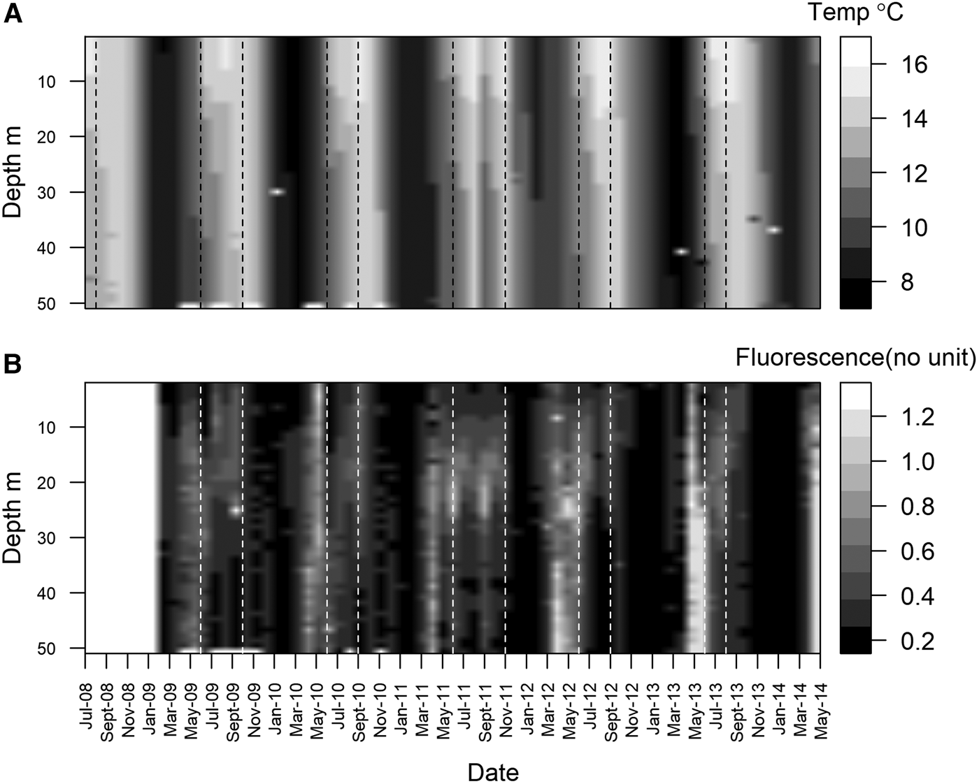
Fig. 1. Monthly mean water temperature (A), between July 2008 and May 2014 and fluorescence (B) between Jan 2009 and May 2014 at station L4. Data were collected weekly (weather permitting) using a SeaBird SBE 19 + CTD deployed from the RV ‘Plymouth Quest’. Dotted vertical lines denote periods of thermal stratification.
Animal collection and processing
Using a 60 cm wide Naturalist dredge with a 22 mm mesh, three replicate samples were taken every other month during the period July 2008–May 2014 from Station L4. For each replicate the dredge was lowered to the seabed and then towed for ~2 min at a speed of ~0.3 knots. Total towed distance was calculated for each replicate using the formula:
 $$\eqalign{&\cos ^{-1}\,(\cos {\rm la}{\rm t}_{\rm S}\; \; \times \cos \; {\rm la}{\rm t}_{\rm E}\; \; + \sin {\rm la}{\rm t}_{\rm S}\; \times \sin {\rm la}{\rm t}_{\rm E}\; \; \times \cos \,({\rm lon}_{\rm S}\,\;\cr & \hfill -\,\; {\rm lon}_{\rm E}))\, \times 6371}$$
Where: latS is start latitude (in radians), latE is end latitude (in radians), lonS is start longitude (in radians), lonE is end longitude (in radians) and 6371 is the approximate radius of the Earth (in km).
All organisms collected in the dredge were fixed in 10% formalin solution. Prior to analysis, samples were rinsed at 4 mm and epifaunal individuals carefully picked out. All individuals were identified to species level, wherever possible, using a stereo microscope (Leica M32 Kombistereo). Individuals within each of the identified taxonomic groups were counted, carefully blotted dry and weighed on a Sartorius R220D microbalance (± 0.01 mg, European Instruments). Standardized values for abundance and biomass for each time point were calculated by dividing the total abundance (or biomass) in three replicate samples by the total area covered by the dredge. Those species which were only ever represented by a single individual across the course of the time series (N = 23) were excluded from further analysis.
Ancillary data
During the study period (July 2008–May 2014), a suite of environmental and biological data were collected from L4 every week (weather permitting) from the RV ‘Plymouth Quest’. Vertical profiles of temperature and fluorescence were measured using a SeaBird SBE 19+ CTD. Water samples for phytoplankton analysis were collected from a depth of 10 m using 10 L Niskin bottles attached to the CTD rosette, and zooplankton were collected in two vertical WP2 net hauls (mesh size = 200 µm, mouth aperture = 57 cm diameter) taken from the seabed to the surface (UNESCO, 1968).
Phytoplankton analysis
Paired water-bottle samples were preserved with 2% Lugol's iodine solution (Throndsen, Reference Throndsen1978) and 4% buffered formaldehyde. Between 10 and 100 ml of sample (depending on cell density) were settled for at least 48 h (Widdicombe et al., Reference Widdicombe, Eloire, Harbour, Harris and Somerfield2010). Cell volumes were calculated according to the equations of Kovala & Larrance (Reference Kovala and Larrance1966) and converted to carbon (pgC cell−1) (Menden-Deuer & Lessard, Reference Menden-Deuer and Lessard2000) and then expressed per unit volume of seawater (mgC m−3).
Meroplankton analysis
Haul samples were preserved and stored in 5% formalin. Two subsamples were extracted using a Folsom splitter and a Stempel pipette, to identify large and small organisms separately, then counted and identified under a microscope. Abundances in the two hauls were averaged to reduce the variability related to the sampling, and counts were converted to individuals per m3 (John et al., Reference John, Batten, Harris and Hays2001). Due to the difficulties in larval identification and because different analysts have worked on the data set over the years, meroplankton are only identified to major taxonomic groups. These groups are: Decapoda, Brachyura, Cirripedia, Bivalvia, Gastropoda, Echinodermata and Polychaeta. These groups provide an overall picture of the seasonal changes in the meroplankton assemblage at L4. For this study, all groups except Cirripedia were considered, because although Cirripede larvae can dominate the meroplankton at L4 (Highfield et al., Reference Highfield, Eloire, Conway, Lindeque, Attrill and Somerfield2010), mature animals are rarely present in the epibenthic faunal samples.
Statistical analysis
All statistical analyses were conducted in R statistical software. Time series of epibenthic abundance and wet biomass per square metre between July 2008 and May 2014 were compiled. Missing data were interpolated using the ‘zoo' package in R (Zeileis et al., Reference Zeileis, Grothendieck, Ryan, Ulrich and Andrews2018). Data for each sampling month (January, March, May, July, September and November) were pooled across the whole time series and overall means of community, major phyla and dominant species abundance and wet biomass were calculated to establish the structure of the community. Average individual body mass of the whole community and each phylum was calculated by dividing the overall mean wet biomass by the overall mean abundance for each sampling month. To establish whether responses to environmental drivers were more easily identifiable when considering functional groups rather than taxa, species were grouped into one of five feeding guilds (predator/scavenger, omnivore, surface-deposit feeder, subsurface-deposit feeder, suspension feeder). Information on polychaete feeding mode was retrieved from Jumars et al. (Reference Jumars, Dorgan and Lindsay2015). Information on feeding mode for all other phyla was retrieved from the Marine Life Information Network's biological traits catalogue (MarLIN, 2006). Where a species exhibited more than one feeding method, it was classified by the preferred or most frequently documented method. While we appreciate that the ‘fuzzy coding’ method (Chevene et al., Reference Chevene, Doléadec and Chessel1994; Neumann & Kröncke, Reference Neumann and Kröncke2011), which uses positive scores to describe the affinity of species to trait categories, would reflect a wider range of ecological function than the method adopted here, the aim of the present study was to provide a broad overview of the structure of the community and its responses to environmental variables, rather than an in-depth analysis of biological traits. Data on meroplanktonic larval abundance, water temperature and phytoplankton carbon for the duration of the time series were also collected and monthly means calculated.
The ‘vegan’ package in R (Oksanen et al., Reference Oksanen, Blanchet, Friendly, Kindt, Legendre, McGlinn, Minchin, O’Hara, Simpson, Solynes, Stevens, Szoecs and Wagner2017) was used to construct a species accumulation curve to determine whether the full diversity of Station L4 had been captured, and to calculate rarefied species richness as an indicator of changes in diversity over the course of the time series. Rarefied species richness was chosen as the measure of diversity as the total area covered by the dredge varied between sampling dates. As a consequence, it is likely that the number of species (and individuals) collected in each sample was a function of the area sampled. Rarefaction techniques can correct for this difference in sampling effort by generating the expected number of species in a small collection of n individuals drawn at random from a larger pool of N individuals (Gotelli & Colwell, Reference Gotelli and Colwell2001).
In order to identify any correlation between the biological (community, feeding guild and phyla abundance and biomass) and the environmental (water temperature, phytoplankton carbon) data series, cross correlation analysis was performed (Olden & Neff, Reference Olden and Neff2001; Probst et al., Reference Probst, Stelzenmüller and Fock2012) in R using the ‘astsa’ package (Stoffer, Reference Stoffer2016). Where relationships between data series were found, linear regressions were used to quantify the relationship for a particular time lag. Cross correlation analysis was also performed on the phyla abundance and larval abundance data series. Prior to this analysis, all data series were checked for homoscedasticity by fitting a simple ordinary least squares regression model and checking the residuals against the fitted values. The community abundance and biomass series, and the larval abundance data series were found to be heteroscedastic and were log-n transformed to achieve homoscedasticity. All data series were differenced to remove any trends or seasonal effects (Probst et al., Reference Probst, Stelzenmüller and Fock2012), and then checked for stationarity using an Augmented Dickey–Fuller test in the ‘tseries’ package for R (Trapletti et al., Reference Trapletti, Hornik and LeBaron2017). Finally, to ensure that estimates of cross correlations were not inflated by any temporal autocorrelation, series were checked for any autocorrelation by generating ACF and PACF plots (Olden & Neff, Reference Olden and Neff2001).
Results
Variations in the epibenthic community 2008–2014
The total area covered by the dredge across the three replicate samples varied from 326.1 m2 in March 2009 to 1170.3 m2 in September 2012. A total of 169 species were recorded over the course of the series, 143 of which were used for analysis. The number of species represented by only a single individual in each sample ranged from 4 (17% of total species recorded in the sample) in January 2012 to 23 (38% of total species recorded in the sample) in July 2009. The species accumulation curve for Station L4 started to level off after ~20 samples (corresponding to a sampling period of 2.5 years) had been collected (Figure 2A). Rarefied species richness varied across the course of the series (Figure 2B) with values ranging from 7–24 species. Spring/summer values were generally higher than values in the preceding winter. Rarefied richness reached a maximum in spring/summer 2011, and declined steadily to the end of the series.
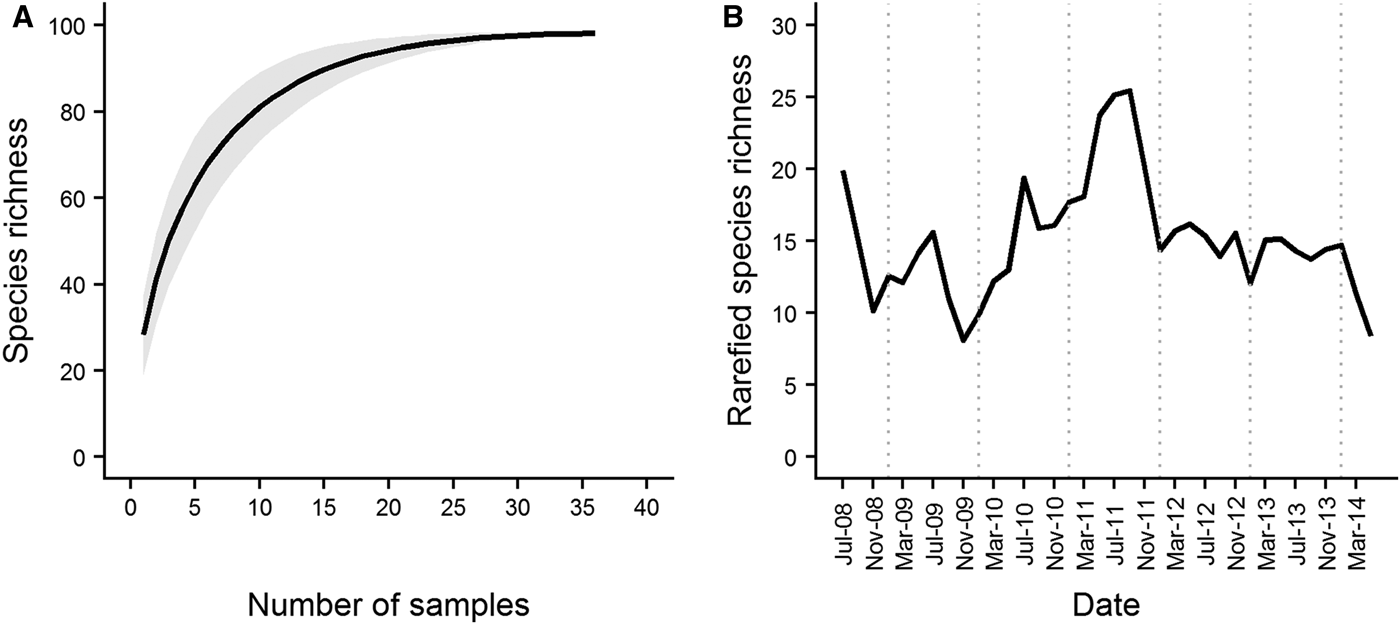
Fig. 2. Species accumulation curve (A) and rarefied species richness (B) over the course of the L4 epibenthic time series, July 2008–May 2014. The species accumulation curve started to level off after ~20 samples (representing a sampling period of 2.5 years) were collected. Grey shading denotes standard deviation from the mean curve, generated from 1000 random permutations of the data. In terms of diversity, the series is characterized by a period of high species richness in late 2010/2011, with periods of lower richness at the beginning and end of the series. Dotted vertical lines denote January of each year.
Community abundance over the course of the series varied from 0.13 individuals m−2 in May 2010, to 3.93 individuals m−2 in May 2014 (Figure 3A). Community wet biomass ranged from 0.21 g m−2 in September 2008 to 5.99 g m−2 in May 2014 (Figure 3B). The peak in community abundance seen in summer 2009 was largely attributable to a peak in crustacean abundance (Figure 3E). The increase in abundance in autumn 2013 was driven by increases in crustaceans (Figure 3E), molluscs (Figure 3E) and to a lesser extent, echinoderms (Figure 3C). The abundance maximum in spring 2014 was due predominantly to an increase in mollusc numbers (Figure 3E). All but one of the observed peaks in wet biomass were driven by increases in echinoderm biomass (Figure 3F). The very high wet biomass maximum in spring 2014 can be attributed to increases in biomass of molluscs and crustaceans (Figure 3F). The increase in polychaete biomass in spring 2014 (Figure 3D) was due to the presence of a single large Aphrodita aculeata (Linnaeus 1758) in the sample. The species which contribute to these peaks in community abundance and biomass are listed in Table 1.

Fig. 3. Abundance of the whole L4 epibenthic community (A), polychaetes and echinoderms (C) and molluscs and crustaceans (E) over the study period July 2008–May 2014. Biomass of the whole community (B), polychaetes (D) and echinoderms, molluscs and crustaceans (F) over the same period. Dotted vertical lines denote January of each year.
Table 1. Species contributing to the observed community and/or wet biomass peaks

Benthic larvae were always present in the water column over the course of the time series. Abundances ranged from 12 (± 8) individuals m−3 in December 2009 to 2080 (± 3656) individuals m−3 in July 2010. In 2009, 2010 and 2011, summer abundances of benthic larvae were very high, reaching more than 1000 individuals m−3 (Figure 4A). In 2009, the majority of the benthic larvae recorded were gastropod molluscs (Figure 4C), while in 2010 and 2011, echinoderm larvae were the primary contributors to the observed peaks in abundance (Figure 4D).

Fig. 4. Abundance of benthic larvae in the water column for (A) the four major benthic phyla, (B) polychaetes, (C) molluscs, (D) echinoderms and (E) decapod crustaceans during the study period July 2008–May 2014. The grey dotted line in panel (C) is the abundance of gastropod larvae present, while the grey dashed line is the abundance of bivalve larvae. The grey dotted line in panel (E) is the abundance of brachyuran larvae present. Grey shading represents standard deviation from the mean calculated for the phyla.
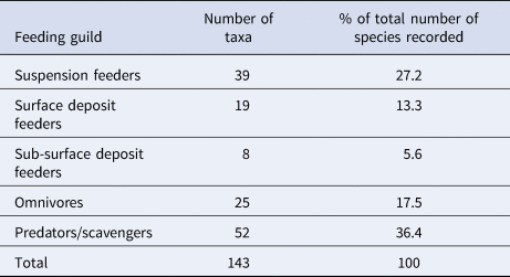
Both the abundance and wet biomass of suspension and deposit feeders was relatively stable over the course of the time series, although suspension feeder abundance increased sharply in summer 2013 and spring 2014 (Figure 5A). Likewise, the wet biomass of suspension and deposit feeders reached a peak in spring 2014 (Figure 5B). In terms of abundance, omnivores were the most dominant feeding guild at L4 (Figure 5C), while the predator/scavenger guild dominated in terms of wet biomass (Figure 5F). The predators/scavengers (Figure 5E) exhibited an increase in abundance in spring 2014, although it was not as dramatic as that recorded for the suspension feeders. The number of taxa mapped into each feeding guild is shown in Table 2. The majority of taxa recorded were predators/scavengers, while sub-surface deposit feeders were represented by only a small number of taxa.
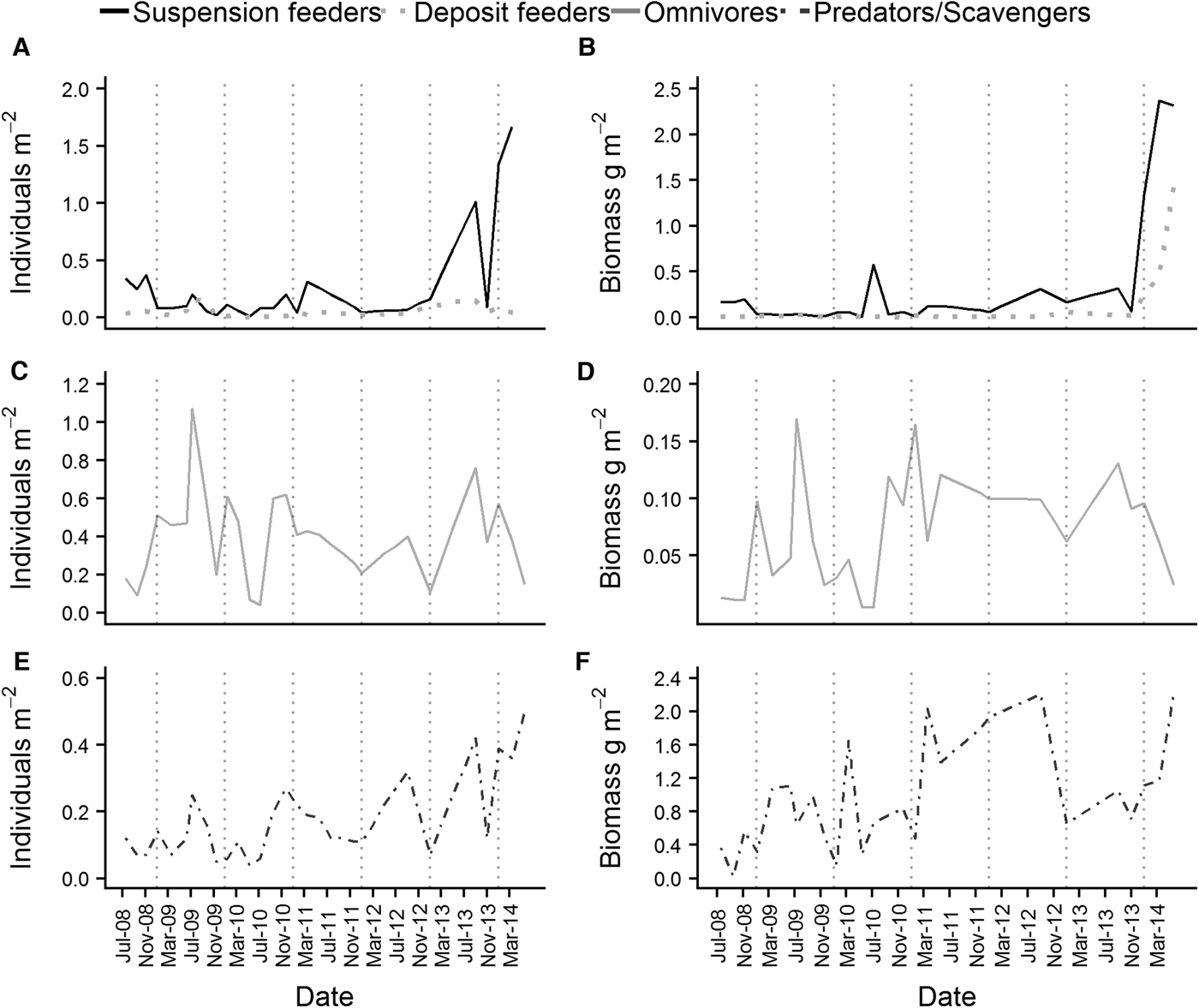
Fig. 5. Abundance (left hand side of the panel) and wet biomass (right hand side of the panel) of the main feeding guilds found at L4. (A) and (B) are suspension and deposit feeders, (C) and (D) are omnivores and (E) and (F) are predators/scavengers. Deposit feeders were split into surface and sub-surface feeders for the purposes of analysis, but were combined for plotting.
Table 2. The number of taxa mapped into each feeding guild and their % contribution to overall species richness
Sub-surface deposit feeders are likely to be under-represented in samples due to the sampling method.
Overall structure of the epibenthic community
There was some structure apparent in the overall means of the community abundance and wet biomass series. Abundance increased from January to reach a peak in May, before declining again over the summer. There was a second, smaller increase apparent in September, and abundance then decreased steadily through the winter (Figure 6A). Wet biomass peaked in March, and remained fairly high over the spring before declining from May onward. There was a second, smaller increase in community wet biomass in September (Figure 6B). The first peak in abundance can be attributed to an increase in abundance of molluscs (Figure 6E) which, when added to an already high abundance of crustaceans (Figure 6I), raised community abundance to ~1.2 individuals m−2. While mollusc abundance dropped sharply after the May maximum (Figure 6E), the decline in community abundance was more gradual, due to an increase in the abundance of crustaceans (Figure 6I), and numbers of polychaetes and echinoderms remaining relatively high (Figure 6C and G). This increase in crustacean abundance, which reached its maximum in September, was the primary contributor to the second community abundance peak (Figure 6A). The biomass maximum in March was predominantly caused by a sharp increase in biomass of echinoderms (Figure 6H), and polychaetes (Figure 6D). Both molluscs and crustaceans (Figure 6F and J) reached a biomass peak in May, ensuring that community biomass remained high throughout the spring (Figure 6B).
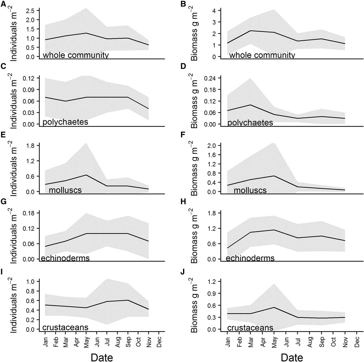
Fig. 6. Overall means for community and major phyla abundance (left hand side of panel) and wet biomass (right hand side of panel), calculated from data for each sampling month (Jan, Mar, May, Jul, Sept, Nov) pooled across the whole time series. Shaded grey area represents standard deviation of the mean.
Average individual body mass of the whole community reached a maximum in March, and then decreased steadily over the summer, before increasing again from September (Figure 7A). Polychaete (Figure 7A) individual body mass exhibited a similar pattern, although the decline after March was much steeper. Peaks in body mass for crustaceans and molluscs (Figure 7A) were reached in May, again with a decrease over the summer, and an increase beginning in September. Echinoderms (Figure 7B) reached a maximum in March, and body mass remained high into May before declining. There was a subsequent increase in echinoderm body mass although it started earlier than in other taxa, in July.
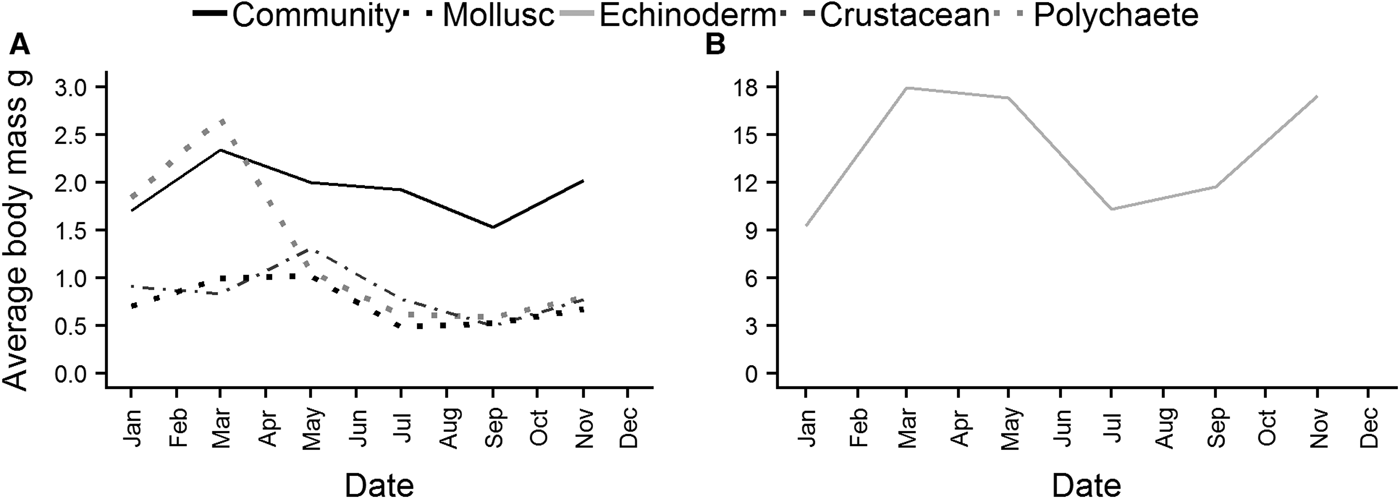
Fig. 7. Average individual body mass of the whole epibenthic community, molluscs, polychaetes and crustaceans (A), and echinoderms (B).
Overall monthly means of larval abundance show that the highest numbers of benthic larvae are recorded in the water column in July/August (Figure 8A). While all four major phyla contribute to this peak in abundance, it is largely attributable to high abundances of molluscs (Figure 8C) and echinoderms (Figure 8D). Different classes of mollusc appear to have different spawning times at L4, with gastropod larvae abundances (grey dotted line, Figure 8C) in the water column peaking slightly earlier than bivalve larvae (grey dashed line, Figure 8C). Polychaete larvae exhibited two peaks, in March and June (Figure 8B), while decapod larvae abundances peaked in March/April (Figure 8E), and remained relatively high throughout the summer, before declining steadily from July. Much of the initial peak in decapod larval abundance can be attributed to brachyuran larvae (grey dotted line, Figure 8E), although this declines after April.
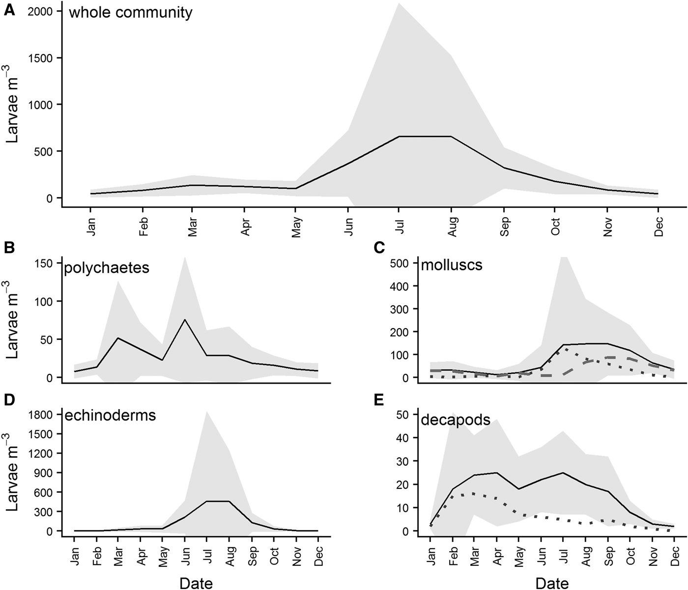
Fig. 8. Overall monthly mean abundances of benthic larvae in the water column for (A) the four major benthic phyla combined, (B) polychaetes, (C) molluscs, (D) echinoderms and (E) decapod crustaceans. Means were calculated for each month from data pooled across the whole time series. The grey dotted line in panel (C) is the abundance of gastropod larvae present, while the grey dashed line is the abundance of bivalve larvae. The grey dotted line in panel (E) is the abundance of brachyuran larvae present. Grey shading represents standard deviation from the mean calculated for the phyla.
Drivers of variation in epibenthic community structure
NMDS ordination revealed no clear seasonal pattern over the course of the time series in either the abundance or wet biomass data, but there were some inter-annual differences in the abundance data. Analysis of community abundance identified three clusters (Figure 9A). Cluster 1 consists of the years 2008, 2013 and 2014. Cluster 2 contains the years 2011 and 2012, and cluster 3 contains the years 2009 and 2010. The differences between these three clusters were driven by differences in the relative abundances of the two dominant species. In cluster 1, the gastropod T. communis was dominant, whereas in cluster 3 the anomuran crab Anapagurus laevis was dominant. Cluster 2 was characterized by a more even community structure, with no single species dominant. There were no clear inter-annual patterns identified in the biomass data, with most data points falling into a single cluster (Figure 9B). The only months to fall outside this cluster were January 2010 and January 2011. This appears to be due to the fact that during these months, the asteroid M. glacialis, which dominated the biomass over the course of the time series, was not recorded.
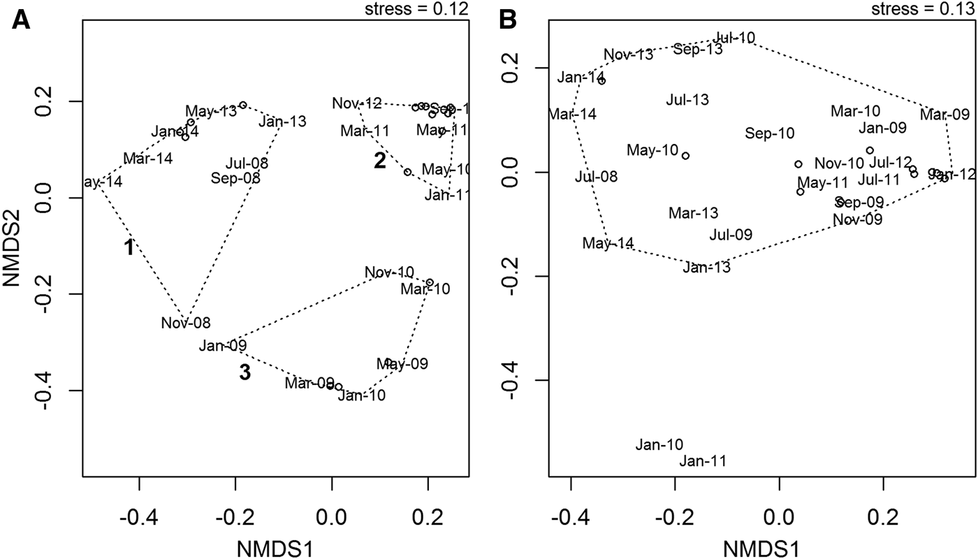
Fig. 9. NMDS ordination of community abundance (A) and wet biomass (B) data over the course of the time series July 2008–May 2014. Although there is no seasonal pattern evident in either the abundance or wet biomass data, there is some inter-annual variation in the abundance data, predominantly due to the relative variations in abundance of the dominant species.
All significant results of the cross correlation analysis are shown in Table 3. There was no significant relationship between total community abundance and any of the explanatory environmental variables. Community wet biomass correlated with both phytoplankton carbon and temperature, with a 6 month lag in both cases. If both carbon and temperature are left in the linear model as explanatory variables, the model fit improves and both terms remain significant. There was no significant interaction effect detected between carbon and temperature. Of the four major phyla, only echinoderm biomass exhibited significant relationships with any of the explanatory environmental variables, correlating with temperature with a 6 month lag. Both mollusc and echinoderm abundance were correlated with larval abundance. Mollusc abundance was correlated with total mollusc larval abundance and gastropod larval abundance with a 4.5 year lag in each case. Echinoderm abundance is correlated with echinoderm larval abundance with a lag of 3 years.
Table 3. Significant models identifying relationships between the epibenthic community and environmental variables. In those models where two predictors were included, the significance value for the whole model has been given in the column for R 2, and the significance value for individual predictors has been given in the coefficients column
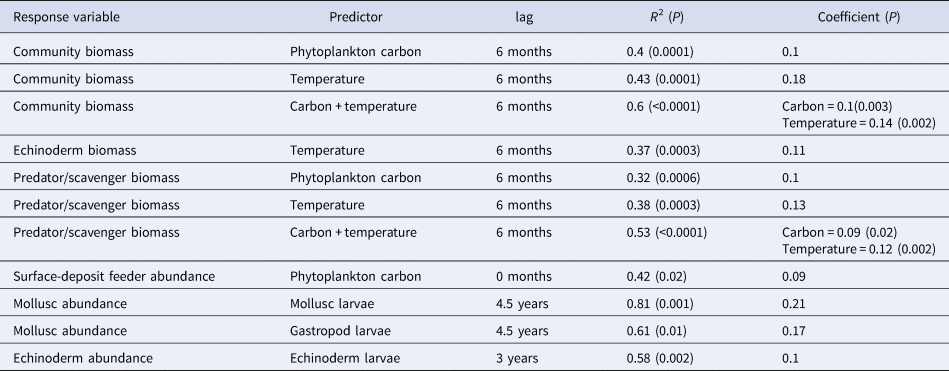
Analysis of the community when grouped into feeding guilds (suspension feeders, surface and sub-surface deposit feeders, omnivores and predators/scavengers) showed a relationship between predator/scavenger biomass and phytoplankton carbon with a 6 month lag (Table 3). As with community wet biomass, this group also exhibited a relationship with temperature, again with a 6 month lag. If both of these terms are left in the model, they remain significant and the overall fit improves (Table 3). There was no significant interaction effect detected however. This analysis also showed a relationship between phytoplankton carbon and surface-deposit feeder abundance, with an immediate response from the surface-deposit feeders to phytodetrital input (Table 3).
Discussion
Time series data (collected every other month during the period July 2008–May 2014) for benthic epifauna at Station L4 were analysed to establish patterns in community abundance, wet biomass and composition, and to link any observed patterns to environmental variables. A clear response to the input of organic material from phytoplankton blooms was detected, with sediment surface living deposit feeders showing an immediate increase in abundance, while predators and scavengers responded later, with an increase in biomass. An inter-annual change in community composition was also detected, as the community shifted from one dominated by the anomuran Anapagurus laevis to one dominated by the gastropod Turitella communis.
There is some evidence for benthic-pelagic coupling at Station L4, demonstrated by the correlation between surface-deposit feeder abundance and phytoplankton carbon. This pattern has been previously observed in the macro-infauna at L4, with deposit feeders rapidly responding to phytodetrital input with an increase in abundance, while predators and scavengers responded more slowly with an increase in biomass (Zhang et al., Reference Zhang, Warwick, McNeill, Widdicombe, Sheehan and Widdicombe2015). While many studies have concluded that benthic communities can be structured by phytodetrital input over both short-term and decadal scales (Buchanan, Reference Buchanan1993; Josefson et al., Reference Josefson, Jensen and Ærtebjerg1993; Dauwe et al., Reference Dauwe, Herman and Heip1998; Wieking & Kröncke, Reference Wieking and Kröncke2005; Frid et al., Reference Frid, Garwood and Robinson2009a, Reference Frid, Garwood and Robinson2009b; Clare et al., Reference Clare, Spencer, Robinson and Frid2017) clear responses to organic input from benthic fauna can be difficult to detect (Graf et al., Reference Graf, Bengtsson, Diesner, Schulz and Theede1982; Reiss & Kröncke, Reference Reiss and Kröncke2004). The ‘food bank’ hypothesis suggests that large reserves of labile organic matter in sediments can sustain benthic communities at constant levels of abundance on a year round basis, and clear responses to phytodetrital input are difficult to detect as a consequence (Mincks et al., Reference Mincks, Smith and DeMaster2005; Kędra et al., Reference Kędra, Kuliński, Walkusz and Legeżyńska2012; Włodarska-Kowalczuk et al., Reference Włodarska-Kowalczuk, Górska, Deja and Morata2016). This appears not to be the case at Station L4, which is fairly impoverished in terms of organic matter content, with organic carbon contributing only 0.4% to total sediment mass (Zhang et al., Reference Zhang, Warwick, McNeill, Widdicombe, Sheehan and Widdicombe2015). It is possible that this comparatively low sediment carbon content results in the epibenthic community at L4 being food limited, and so the seasonal pulses of phytodetrital input elicit measurable responses. Furthermore, spring bloom sedimentation in temperate areas can often occur when bottom water temperatures are low, and benthic faunal responses are limited as a result. Weeks can pass before water temperature increases enough to allow for macrofaunal feeding (Lopez & Levinton, Reference Lopez, Levinton, Wolanski and McLusky2011). It is possible that the particular hydrographic conditions in the Western English Channel, where bottom water temperatures fluctuate less than in other temperate systems, result in early spring temperatures high enough for the surface-deposit feeders in the L4 community to respond immediately.
Interestingly, there was no apparent decrease in diversity associated with the sedimentation of the spring bloom. In macrofaunal communities, enriched sediments are typically rapidly colonized by a few opportunist, fast-reproducing species (Widbom & Frithsen, Reference Widbom and Frithsen1995) which can take advantage of the fresh organic matter, generally resulting in a reduction in diversity (Chamberlain et al., Reference Chamberlain, Fernandes, Read, Nickell and Davies2001; Widdicombe & Austen, Reference Widdicombe and Austen2001). As noted above, epibenthic surface-deposit feeders did show an immediate increase in abundance with the arrival of phytodetritus, but rarefied richness values for May (post sedimentation) are generally equal to or higher than values for March (pre-bloom). It is possible that these values are indirect evidence of predation. Predation is thought to play a key role in marine sedimentary systems, due in part to the lack of clear evidence for competitive exclusion (Peterson, Reference Peterson and Livingston1979; Woodin, Reference Woodin1999). While detection of predation is challenging, and numerous studies have found no consistent regulatory role (Thrush, Reference Thrush1999), it has been suggested that epibenthic predators can equalize numbers and increase evenness by preying preferentially on numerically dominant species (Quijón & Snelgrove, Reference Quijón and Snelgrove2005). Given the fact that L4 community wet biomass is predominantly represented by predators and scavengers, there is a possibility that opportunistic deposit feeders are prevented from becoming dominant after sedimentation of the spring bloom by the feeding of the predator/scavenger group. This pattern in the regulation of benthic community structure has been noted before (Posey et al., Reference Posey, Powell, Cahoon and Lindquist1995), with those authors concluding that the presence or absence of predation may alter the visible response of the benthos to organic enrichment. While there was no direct evidence of predator–prey interactions (e.g. a clear relationship between deposit-feeder and predator/scavenger abundance or biomass, as defined by Lotka–Volterra type models) detected in this study, the patterns in species richness observed would seem to support the proposal that epibenthic predators can be of major influence in benthic communities (Quijón & Snelgrove, Reference Quijón and Snelgrove2005), and may diminish or counterbalance the changes in prey species that result from phytodetrital input.
A relationship between community wet biomass and both bottom-water temperature and phytoplankton carbon was detected at Station L4, although there was no significant interaction between the two predictors and their effects on biomass. This leads us to propose that temperature and phytoplankton carbon primarily influence biomass at different times of the year. Community wet biomass peaks in March/May, driven predominantly by an increase in biomass of echinoderms and molluscs. Individual body mass curves for these two phyla show an identical pattern, with a maximum also being reached in March/May. It is possible that this is representative of the development of the gonads in preparation for spawning. Several studies have found that ripe gonads in these two phyla can make a significant contribution to body mass (Barker & Nichols, Reference Barker and Nichols1983; Nichols & Barker, Reference Nichols and Barker1984a, Reference Nichols and Barker1984b; Berthelin et al., Reference Berthelin, Kellner and Mathieu2000; Freeman et al., Reference Freeman, Richardson and Seed2001; Alunno-Bruscia et al., Reference Alunno-Bruscia, Bourlès, Maurer, Robert, Mazurié, Gangnery, Goulletquer and Pouvreau2011). This view would appear to be supported by the increase in benthic larvae (of which mollusc and echinoderm larvae are recorded in the highest numbers) in the water column from May onwards, while community, mollusc and echinoderm biomass decreases after May, perhaps indicating spent individuals. We suggest that this pre-spawning biomass is influenced by temperature. Several studies have noted the role of temperature in triggering gonad development in marine invertebrate species (Sastry, Reference Sastry1966; Sastry & Blake, Reference Sastry and Blake1971; Aktaş et al., Reference Aktaş, Kumlu and Eroldogan2003; Herrmann et al., Reference Herrmann, Alfaya, Lepore, Penchaszadeh and Laudien2009; Balogh et al., Reference Balogh, Wolfe and Byrne2018), and it is possible that gonad development at L4 is initiated by the high water temperatures recorded in September, with full maturation and spawning occurring the following spring. Gonad development and maturation in some temperate echinoderm and mollusc species has been recorded to take up to 6 months, which would be in keeping with the 6-month lag between peaks in temperature and biomass identified in this study (Bowner, Reference Bowner1982; Sköld & Gunnarsson, Reference Sköld and Gunnarsson1996; Kim et al., Reference Kim, Kim, Son, Jeon, Lee and Lee2016). Although there was no significant interaction between temperature and phytoplankton carbon and their effects on biomass detected in this study, food availability will clearly affect gonad development as it dictates the nutritional status of an individual (Nunes & Jangoux, Reference Nunes and Jangoux2004), and the autumn bloom characteristic of Station L4, along with the carbon from seaweed detritus which contributes to winter organic matter in the area (Queirós et al., Reference Queirós, Stephens, Widdicombe, Tait, McCoy, Ingels, Rühl, Airs, Beesley, Carnovale, Cazenave, Dashfield, Hua, Jones, Lindeque, McNeill, Nunes, Parry, Pascoe, Widdicombe, Smyth, Atkinson, Krause-Jensen and Somerfield2019) is likely to help fuel gonad development over the winter. In contrast to maximum temperatures, maximum phytoplankton carbon values are generally recorded in April/May, with a response in community biomass seen 6 months later. It is possible that the relationship between phytoplankton carbon and biomass is indicative of somatic growth, which occurs after spawning has taken place in the spring. The seasonal prioritization of either sexual or somatic growth in benthic fauna is well documented, particularly in echinoderms (Greenwood, Reference Greenwood1980; Peterson & Fegley, Reference Peterson and Fegley1986; Guillou & Michel, Reference Guillou and Michel1993; Lozano et al., Reference Lozano, Galera, López, Turon, Palacín and Morera1995; Coma et al., Reference Coma, Ribes, Gili and Zabala1998). This shift in energetic prioritization is often related to reproductive effort being concentrated at a time favourable to the survival of offspring, e.g. spawning prior to or coincident with a phytoplankton bloom (Giangrande et al., Reference Giangrande, Geraci and Belmonte1994). The same lagged relationship between biomass, temperature and phytoplankton carbon was also recorded in the predator/scavenger group. The biomass of this feeding guild is dominated by echinoderms (70%), so the postulated relationships outlined above could also be driving the responses of this group.
The role of larval supply as a determinant of the structure and dynamics of marine populations (i.e. supply side ecology) has long been discussed (Thorson, Reference Thorson1950; De Wolf, Reference De Wolf1973; Lewin, Reference Lewin1986; Underwood & Fairweather, Reference Underwood and Fairweather1989), and there is much evidence to suggest that variations in recruitment can contribute to patterns of abundance and demographics in adult populations of fish (Williams, Reference Williams1980; Doherty & Fowler, Reference Doherty and Fowler1994), barnacles (Gaines & Roughgarden, Reference Gaines and Roughgarden1985; Sutherland, Reference Sutherland1990; Scrosati & Ellrich, Reference Scrosati and Ellrich2017), mussels (Scrosati & Ellrich, Reference Scrosati and Ellrich2017) and bryzoans (Hughes, Reference Hughes1990). We propose that larval recruitment of dominant species is also a key influence on benthic community structure and composition at Station L4. The dramatic increase in community and suspension feeder abundance and biomass in May 2014, and the shift in community structure (from one dominated by Anapagurus laevis in 2009 to one dominated by T. communis in 2013/2014) are likely due to the sieve recruitment (the point at which individuals recruited to the population reach a size where they would be retained on the sieve mesh) of the high numbers of gastropod larvae present in the plankton in 2009. Previous studies of benthic recruitment have stressed that sieve recruitment can be far removed in time from actual settlement (Buchanan & Moore, Reference Buchanan and Moore1986), as many benthic macrofaunal settlers are of meiofaunal size. The lag of 4.5 years identified between mollusc abundance and gastropod larval abundance likely reflects the fact that any newly settled animal needs to reach a size both big enough to be collected by the dredge, and to be retained on the 4 mm sieve used in this study.
Analysis of the first six years of the epibenthic time series at Station L4 reveals some temporal structure in community abundance and wet biomass, apparently influenced by both bottom water temperature and seasonal phytodetrital input. We suggest that the spring phytoplankton bloom fuels somatic growth, while gonad development and maturation is triggered by warmer water temperature in the autumn, resulting in a pre-spawning biomass peak evident in early spring. Different functional groups within the community were found to respond to the bloom in specific ways, a result that is in keeping with previous studies of the L4 macro-benthos. While benthic faunal responses to changes in water temperatures have been previously recorded in other temperate systems, clear responses to phytodetrital input as seen here are less common. We suggest that the reason we can detect this response is a combination of two factors. (1) The relative impoverishment of the L4 sediment in terms of organic content, indicating a food-limited community, and (2) the comparatively small range of bottom water temperatures, resulting in relatively mild winter/early spring conditions and a community that is able to take immediate advantage of bloom sedimentation.
Acknowledgements
We are grateful to the crew of the RV ‘Plymouth Quest’, Sarah Dashfield, Joana Nunes, Amanda Beesley and Louise McNeill for benthic sample collection; Adrien Lowenstein, Laura Briers, Bianca Maria Torre, Harry Powell, Alessandro Brunzini, Craig Dornan, Olli Ford and Jemma French for their contributions to the taxonomic analysis of the benthic epifaunal samples; Clare Widdicombe for providing the phytoplankton data, and Andrea McEvoy and Angus Atkinson for providing the meroplankton data. We would also like to thank the two anonymous reviewers whose comments improved the manuscript considerably.
Financial support
This work was supported by the National Environment Research Council via the SPITFIRE studentship [E.T., grant number NE/L002531/1] and through its National Capability Long-term Single Centre Science Programme, Climate Linked Atlantic Sector Science [grant number NE/R015953/1], and is a contribution to Theme 1.3 – Biological Dynamics.


