


1 Introduction
Equivalence relations on countable structures are among the most heavily studied objects in descriptive set theory and computability theory. In descriptive set theory, starting with the work of Friedman and Stanley [Reference Friedman and Stanley10], the complexity of equivalence relations on spaces of structures under Borel reducibility has seen much interest by experts, culminating in results by Louveau and Rosendal [Reference Louveau and Rosendal16], who showed that, among others, the bi-embeddability relation on graphs is $\boldsymbol {\Sigma }^1_1$
-complete. Since then there has been a constant stream of work on the complexity of the bi-embeddability relation, both on other classes of structures, see for instance [Reference Calderoni and Thomas4], and refinements of completeness notions, e.g., in [Reference Camerlo, Marcone and Ros5].
$\boldsymbol {\Sigma }^1_1$
-complete. Since then there has been a constant stream of work on the complexity of the bi-embeddability relation, both on other classes of structures, see for instance [Reference Calderoni and Thomas4], and refinements of completeness notions, e.g., in [Reference Camerlo, Marcone and Ros5].
Equivalence relations are also one of the main objects of study in computability theory. Here, the equivalence relations are usually on the set of natural numbers and their complexity is established using computable reducibility. Identifying a computable structure with the index of the algorithm computing it, one can obtain completeness results like the ones in descriptive set theory for equivalence relations on computable structures [Reference Fokina and Friedman6, Reference Fokina, Friedman, Harizanov, Knight, Mccoy and Montalbán9]. One object of study in computable structure theory which also takes non-computable structures into account is degree spectra of structures, introduced by Knight [Reference Knight15]. The degree spectrum of a given structure is the set of sets of natural numbers Turing equivalent to one of its isomorphic copies. They provide a measure of the algorithmic complexity of countable structures.
Recently, researchers initiated the study of degree spectra with respect to other model theoretic equivalence relations such as bi-embeddability [Reference Fokina, Rossegger and Mauro7], elementary bi-embeddability [Reference Rossegger20], elementary equivalence [Reference Andrews and Knight1–Reference Andrews, Cai, Diamondstone, Lempp and Miller3], or $\Sigma _n$
equivalence [Reference Fokina, Semuhin and Turetsky8]. One of the main goals in this line of research is to distinguish these equivalence relations with respect to the degree spectra they realize. While for elementary equivalence and
$\Sigma _n$
equivalence [Reference Fokina, Semuhin and Turetsky8]. One of the main goals in this line of research is to distinguish these equivalence relations with respect to the degree spectra they realize. While for elementary equivalence and $\Sigma _n$
equivalence examples that separate them from each other and from isomorphism and elementary bi-embeddability are known, so far all attempts to separate isomorphism, bi-embeddability, and elementary bi-embeddability have been unsuccessful.
$\Sigma _n$
equivalence examples that separate them from each other and from isomorphism and elementary bi-embeddability are known, so far all attempts to separate isomorphism, bi-embeddability, and elementary bi-embeddability have been unsuccessful.
There seem to be various reasons for this. That we can separate elementary equivalence and $\Sigma _n$
equivalence is the case because they have different levels in the Borel hierarchy while isomorphism and bi-embeddability are not even Borel. On the other hand bi-embeddability preserves very little structural properties and it is thus difficult to construct interesting examples. The aim of this article is to investigate the relationship between the degree spectra realized by the bi-embeddability relation and by the elementary bi-embeddability relation. First, we establish that elementary bi-embeddability on graphs is
$\Sigma _n$
equivalence is the case because they have different levels in the Borel hierarchy while isomorphism and bi-embeddability are not even Borel. On the other hand bi-embeddability preserves very little structural properties and it is thus difficult to construct interesting examples. The aim of this article is to investigate the relationship between the degree spectra realized by the bi-embeddability relation and by the elementary bi-embeddability relation. First, we establish that elementary bi-embeddability on graphs is $\boldsymbol {\Sigma }^1_1$
complete with respect to Borel reducibility. We then proceed to establish a relationship between the degree spectra realized by the bi-embeddability and elementary bi-embeddability relation on graphs. Our main results are as follows.
$\boldsymbol {\Sigma }^1_1$
complete with respect to Borel reducibility. We then proceed to establish a relationship between the degree spectra realized by the bi-embeddability and elementary bi-embeddability relation on graphs. Our main results are as follows.
Theorem 1.1. The elementary embeddability relation on graphs $\mathbin{\preccurlyeq}_{\mathfrak {G}}$
is a complete
$\mathbin{\preccurlyeq}_{\mathfrak {G}}$
is a complete $\boldsymbol {\Sigma }^1_1$
quasi-order. In particular, the elementary bi-embeddability relation on graphs
$\boldsymbol {\Sigma }^1_1$
quasi-order. In particular, the elementary bi-embeddability relation on graphs $\approxeq _{\mathfrak {G}}$
is a complete
$\approxeq _{\mathfrak {G}}$
is a complete $\boldsymbol {\Sigma }^1_1$
equivalence relation.
$\boldsymbol {\Sigma }^1_1$
equivalence relation.
As a corollary of Theorem 1.1 we obtain the corresponding result for elementary bi-embeddability on computable structures.
Theorem 1.2. The elementary embeddability relation on the class of computable graphs is a $\Sigma ^1_1$
complete quasi-order with respect to computable reducibility. In particular, the elementary bi-embeddability relation on computable graphs is a
$\Sigma ^1_1$
complete quasi-order with respect to computable reducibility. In particular, the elementary bi-embeddability relation on computable graphs is a $\Sigma ^1_1$
complete equivalence relation with respect to computable reducibility.
$\Sigma ^1_1$
complete equivalence relation with respect to computable reducibility.
The following result establishes a relationship between bi-embeddability spectra of graphs and elementary bi-embeddability spectra of graphs.
Theorem 1.3. Let $\mathcal {G}$
be an automorphically non-trivial graph, then there is a graph
$\mathcal {G}$
be an automorphically non-trivial graph, then there is a graph $\hat {\mathcal {G}}$
such that
$\hat {\mathcal {G}}$
such that
 $$ \begin{align*} \textit{DgSp}_\approxeq(\hat{\mathcal{G}})=\{X: X'\in \textit{DgSp}_\approx({\mathcal{G}})\}.\end{align*} $$
Note that in Theorem 1.3 we deal only with automorphically non-trivial graphs. This might seem like a shortcoming; however, automorphically trivial structures are not interesting from a computability theoretic point of view. In particular, every structure bi-embeddable with an automorphically trivial graph is computable and thus both its bi-embeddability spectrum and elementary bi-embeddability spectrum are the set of all computable sets.
The proofs of Theorems 1.1 and 1.2 are the topic of Section 3. In Section 4 we build on these results to prove Theorem 1.3. In Section 2 we give the necessary background and definitions.
2 Background
Our definitions follow for the most part [Reference Gao12, Reference Montalbán19]. We assume that all structures have universe $\omega $
and are relational. Let
$\omega $
and are relational. Let $\mathcal {L}$
be a relational language
$\mathcal {L}$
be a relational language $(R_i)_{i\in \omega }$
where without loss of generality
$(R_i)_{i\in \omega }$
where without loss of generality $R_i$
has arity i. Then each element
$R_i$
has arity i. Then each element $\mathcal {A}$
of
$\mathcal {A}$
of $Mod(\mathcal {L})$
can be viewed as an element of the product space
$Mod(\mathcal {L})$
can be viewed as an element of the product space
 $$ \begin{align*} X_{\mathcal{L}}=\prod_{i\in \omega} 2^{\omega^{i}},\end{align*} $$
and thus $Mod(\mathcal {L})$
becomes a compact Polish space on which we can define the Borel and projective hierarchy in the usual way.
$Mod(\mathcal {L})$
becomes a compact Polish space on which we can define the Borel and projective hierarchy in the usual way.
Let $\mathcal {A}$
be an
$\mathcal {A}$
be an $\mathcal {L}$
-structure and
$\mathcal {L}$
-structure and $(\varphi _i^{at})_{i\in \omega }$
be a computable enumeration of the atomic
$(\varphi _i^{at})_{i\in \omega }$
be a computable enumeration of the atomic $\mathcal {L}$
-sentences with variables in
$\mathcal {L}$
-sentences with variables in $\{x_1,x_2,\dots \}$
. The atomic diagram
$\{x_1,x_2,\dots \}$
. The atomic diagram $D(\mathcal {A})$
of
$D(\mathcal {A})$
of $\mathcal {A}$
is the element of Cantor space defined by
$\mathcal {A}$
is the element of Cantor space defined by
 $$ \begin{align*} D(\mathcal{A})(i)=\begin{cases} 1 & \text{ if } \mathcal{A}\models \varphi_i^{at}[x_j{\rightarrow} j : j\in\omega],\\ 0 &\text{ otherwise.}\end{cases}\end{align*} $$
The Turing degree of a structure $\mathcal {A}$
is the degree of
$\mathcal {A}$
is the degree of $D(\mathcal {A})$
. We will in general not distinguish between a structure as an element of
$D(\mathcal {A})$
. We will in general not distinguish between a structure as an element of $Mod(\mathcal {L})$
and its atomic diagram and assume that what is meant is clear from the context.
$Mod(\mathcal {L})$
and its atomic diagram and assume that what is meant is clear from the context.
Variations of the following definition were independently suggested in [Reference Fokina, Semuhin and Turetsky8, Reference Miller, Poonen, Schoutens and Shlapentokh17, Reference Yu22].
Definition 2.1. Let E be an equivalence relation on $Mod(\mathcal {L})$
and
$Mod(\mathcal {L})$
and $\mathcal {A}\in Mod(\mathcal {L})$
. Then the degree spectrum of
$\mathcal {A}\in Mod(\mathcal {L})$
. Then the degree spectrum of $\mathcal {A}$
with respect to E, or, short E-spectrum of
$\mathcal {A}$
with respect to E, or, short E-spectrum of $\mathcal {A}$
, is the set
$\mathcal {A}$
, is the set
 $$ \begin{align*} \textit{DgSp}_E(\mathcal{A})=\{ X: \exists \mathcal{B} \mathbin{E} \mathcal{A}\ D(\mathcal{B})\equiv_T X\}.\end{align*} $$
We write $\mathcal {A}\mathbin{\hookrightarrow}\mathcal {B}$
to say that
$\mathcal {A}\mathbin{\hookrightarrow}\mathcal {B}$
to say that $\mathcal {A}$
is embeddable in
$\mathcal {A}$
is embeddable in $\mathcal {B}$
, and
$\mathcal {B}$
, and $\mathcal {A}\approx \mathcal {B}$
to say that
$\mathcal {A}\approx \mathcal {B}$
to say that $\mathcal {A}$
is bi-embeddable with
$\mathcal {A}$
is bi-embeddable with $\mathcal {B}$
, i.e.,
$\mathcal {B}$
, i.e., $\mathcal {A}\mathbin{\hookrightarrow}\mathcal {B}$
and
$\mathcal {A}\mathbin{\hookrightarrow}\mathcal {B}$
and $\mathcal {B}\mathbin{\hookrightarrow} \mathcal {A}$
. Further, we write
$\mathcal {B}\mathbin{\hookrightarrow} \mathcal {A}$
. Further, we write $\mathcal {A}\mathbin{\preccurlyeq} \mathcal {B}$
to say that
$\mathcal {A}\mathbin{\preccurlyeq} \mathcal {B}$
to say that $\mathcal {A}$
is elementary embeddable in
$\mathcal {A}$
is elementary embeddable in $\mathcal {B}$
and
$\mathcal {B}$
and $\mathcal {A}\approxeq \mathcal {B}$
to say that
$\mathcal {A}\approxeq \mathcal {B}$
to say that $\mathcal {A}$
is elementary bi-embeddable with
$\mathcal {A}$
is elementary bi-embeddable with $\mathcal {B}$
, i.e.,
$\mathcal {B}$
, i.e., $\mathcal {A}\mathbin{\preccurlyeq} \mathcal {B}$
and
$\mathcal {A}\mathbin{\preccurlyeq} \mathcal {B}$
and $\mathcal {B}\mathbin{\preccurlyeq} \mathcal {A}$
.
$\mathcal {B}\mathbin{\preccurlyeq} \mathcal {A}$
.
Definition 2.2. Let $R,S$
be binary relations on a set X. The relation R is reducible to S if there is a function
$R,S$
be binary relations on a set X. The relation R is reducible to S if there is a function $f: X\mathbin{\rightarrow} X$
such that for all
$f: X\mathbin{\rightarrow} X$
such that for all $x,y\in X$
 $$ \begin{align*} x R y \Leftrightarrow f(x)Sf(y).\end{align*} $$
Assume $X=Mod(\mathcal {L})$
. Then
$X=Mod(\mathcal {L})$
. Then
-
(1) R is Borel reducible to S if f is Borel on $Mod(\mathcal {L})\times Mod(\mathcal {L}) $
,
$Mod(\mathcal {L})\times Mod(\mathcal {L}) $
, -
(2) R is computably reducible to S if there is a computable operator
$\Phi $
such that for all
$\mathcal {A}\in Mod(\mathcal {L})$
,
$\Phi ^{D(\mathcal {A})}=D(f(\mathcal {A}))$
.

Assume X is $\omega $
and that
$\omega $
and that $(\mathcal {A}_i)_{i\in \omega }$
is a computable enumeration of all partial computable
$(\mathcal {A}_i)_{i\in \omega }$
is a computable enumeration of all partial computable $\mathcal {L}$
structures. Then R is computably reducible to S if f is a computable function.
$\mathcal {L}$
structures. Then R is computably reducible to S if f is a computable function.
We say that an equivalence relation (quasi-order) $R\in \Gamma $
is a
$R\in \Gamma $
is a $\Gamma $
complete equivalence relation (quasi-order) for a complexity class
$\Gamma $
complete equivalence relation (quasi-order) for a complexity class $\Gamma $
with respect to x-reducibility if all equivalence relations (quasi-orders) in
$\Gamma $
with respect to x-reducibility if all equivalence relations (quasi-orders) in $\Gamma $
are x-reducible to R.
$\Gamma $
are x-reducible to R.
A standard reference on Borel reducibility is [Reference Gao12]. Computable reducibility on the natural numbers can be seen as a natural effectivization of Borel reducibility where one only considers computable structures. Fokina and Friedman [Reference Fokina and Friedman6] showed that bi-embeddability on trees and thus also graphs is $\Sigma ^1_1$
complete with respect to computable reducibility, and in [Reference Fokina, Friedman, Harizanov, Knight, Mccoy and Montalbán9] it is shown that isomorphism on graphs is
$\Sigma ^1_1$
complete with respect to computable reducibility, and in [Reference Fokina, Friedman, Harizanov, Knight, Mccoy and Montalbán9] it is shown that isomorphism on graphs is $\Sigma ^1_1$
complete with respect to computable reducibility. This contrasts with Borel reducibility; it is well known that isomorphism on graphs is not
$\Sigma ^1_1$
complete with respect to computable reducibility. This contrasts with Borel reducibility; it is well known that isomorphism on graphs is not $\boldsymbol {\Sigma }^1_1$
complete.
$\boldsymbol {\Sigma }^1_1$
complete.
3 Elementary bi-embeddability is analytic complete
In this section we prove Theorems 1.1 and 1.2 and some lemmas needed for Theorem 1.3. The section is structured as follows. In Section 3.1 we give a reduction from embeddability on the class of graphs $\mathfrak {G}$
to elementary embeddability on a Borel class
$\mathfrak {G}$
to elementary embeddability on a Borel class $\mathfrak {C}$
of structures in an infinite relational language. In Section 3.2 we show that graphs are complete for elementary embeddability. That is, for every Borel class, elementary embeddability on this class can be reduced to elementary embeddability on graphs. Theorem 1.1 then follows by composing the reductions given in Sections 3.1 and 3.2. For Theorem 1.2 we need a few more observations made at the end of this section.
$\mathfrak {C}$
of structures in an infinite relational language. In Section 3.2 we show that graphs are complete for elementary embeddability. That is, for every Borel class, elementary embeddability on this class can be reduced to elementary embeddability on graphs. Theorem 1.1 then follows by composing the reductions given in Sections 3.1 and 3.2. For Theorem 1.2 we need a few more observations made at the end of this section.
3.1 The reduction from
$\mathbin{\hookrightarrow}_{\mathfrak {G}}$
to
$\mathbin{\preccurlyeq}_{\mathfrak {C}}$


The main idea of the construction is that for any given graph $\mathcal {G}$
we replace the edge relation with structures having the property that they are minimal under elementary embeddability.
$\mathcal {G}$
we replace the edge relation with structures having the property that they are minimal under elementary embeddability.
Definition 3.1. A structure $\mathcal {A}$
is minimal if it does not have proper elementary substructures.
$\mathcal {A}$
is minimal if it does not have proper elementary substructures.
Minimal structures were investigated by Fuhrken [Reference Fuhrken11] who showed that there is a theory with $2^{\aleph _0}$
minimal models, and Shelah [Reference Shelah21] who showed that for every
$2^{\aleph _0}$
minimal models, and Shelah [Reference Shelah21] who showed that for every $n\leq \aleph _0$
, there is a theory with n minimal models. Later, Ikeda [Reference Ikeda14] investigated minimal models of minimal theories. Notice that a prime model is not necessarily minimal, as it might contain elementary substructures isomorphic to itself.
$n\leq \aleph _0$
, there is a theory with n minimal models. Later, Ikeda [Reference Ikeda14] investigated minimal models of minimal theories. Notice that a prime model is not necessarily minimal, as it might contain elementary substructures isomorphic to itself.
Given a graph $\mathcal {G}$
, if
$\mathcal {G}$
, if $x,y\in G$
and
$x,y\in G$
and $xEy$
, then we associate a copy of a structure
$xEy$
, then we associate a copy of a structure $\mathcal {A}$
with the pair
$\mathcal {A}$
with the pair $(x,y)$
and otherwise we associate a copy
$(x,y)$
and otherwise we associate a copy $\mathcal {B}$
with
$\mathcal {B}$
with $(x,y)$
. The structures
$(x,y)$
. The structures $\mathcal {A}$
and
$\mathcal {A}$
and $\mathcal {B}$
will be elementary equivalent and minimal.
$\mathcal {B}$
will be elementary equivalent and minimal.
Before we formally state the reduction let us describe $\mathcal {A}$
and
$\mathcal {A}$
and $\mathcal {B}$
. They will be models of the theory of the following structure studied by Shelah [Reference Shelah21]. The language of the theory contains countably many unary functions
$\mathcal {B}$
. They will be models of the theory of the following structure studied by Shelah [Reference Shelah21]. The language of the theory contains countably many unary functions $F_\nu $
and unary relation symbols
$F_\nu $
and unary relation symbols $R_\nu $
, one for each
$R_\nu $
, one for each $\nu \in 2^{<\omega }$
. Consider the structure
$\nu \in 2^{<\omega }$
. Consider the structure
 $$ \begin{align*} \mathcal{S}=(2^\omega, \langle F_\nu\rangle_{\nu\in 2^{<\omega}}, \langle R_\nu\rangle_{\nu\in 2^{<\omega}}),\end{align*} $$
where $F_\nu $
is defined by
$F_\nu $
is defined by $F_\nu (\sigma )(x)=\sigma (x)+\nu (x)\mod 2$
where we assume that
$F_\nu (\sigma )(x)=\sigma (x)+\nu (x)\mod 2$
where we assume that $\nu (x)=0$
for
$\nu (x)=0$
for $x\geq |\nu |$
and
$x\geq |\nu |$
and $R_\nu (\sigma )$
if and only if
$R_\nu (\sigma )$
if and only if $\nu \prec \sigma $
. Shelah showed that the theory of
$\nu \prec \sigma $
. Shelah showed that the theory of $\mathcal {S}$
has quantifier elimination and that each element of
$\mathcal {S}$
has quantifier elimination and that each element of $\mathcal {S}$
generates an elementary substructure that is minimal.
$\mathcal {S}$
generates an elementary substructure that is minimal.
Let $\hat {\mathcal {S}_0}$
be the substructure of
$\hat {\mathcal {S}_0}$
be the substructure of $\mathcal {S}$
generated by
$\mathcal {S}$
generated by $\bar 0$
, the constant string of
$\bar 0$
, the constant string of $0$
’s, and
$0$
’s, and $\hat {\mathcal {S}_1}$
be the substructure generated by
$\hat {\mathcal {S}_1}$
be the substructure generated by $\bar 1$
, the constant string of
$\bar 1$
, the constant string of $1$
’s. These structures are countable and by Shelah’s argument,
$1$
’s. These structures are countable and by Shelah’s argument, $\hat {\mathcal {S}}_0\equiv \hat {\mathcal {S}}_1\equiv \mathcal {S}$
. Furthermore,
$\hat {\mathcal {S}}_0\equiv \hat {\mathcal {S}}_1\equiv \mathcal {S}$
. Furthermore, $\hat {\mathcal {S}}_0$
and
$\hat {\mathcal {S}}_0$
and $\hat {\mathcal {S}}_1 $
are minimal models of
$\hat {\mathcal {S}}_1 $
are minimal models of $Th(\mathcal {S})$
. To see this, let
$Th(\mathcal {S})$
. To see this, let $x\in \hat S_0$
, then
$x\in \hat S_0$
, then $x=F_\nu (\bar 0)$
and in particular,
$x=F_\nu (\bar 0)$
and in particular, $\bar 0=F_\nu (x)$
for some
$\bar 0=F_\nu (x)$
for some $\nu \in 2^{<\omega }$
. So, the substructure of
$\nu \in 2^{<\omega }$
. So, the substructure of $\hat {\mathcal {S}}_0$
generated by x is already
$\hat {\mathcal {S}}_0$
generated by x is already $\hat {\mathcal {S}}_0$
.
$\hat {\mathcal {S}}_0$
.
As we require our structures in $\mathfrak {C}$
to be of relational syntax we will let
$\mathfrak {C}$
to be of relational syntax we will let $\mathcal {S}_0$
and
$\mathcal {S}_0$
and $\mathcal {S}_1$
be the structures corresponding to
$\mathcal {S}_1$
be the structures corresponding to $\hat {\mathcal {S}}_0$
, respectively
$\hat {\mathcal {S}}_0$
, respectively $\hat {\mathcal {S}}_1$
, after we replace each
$\hat {\mathcal {S}}_1$
, after we replace each $F_\nu ^{\mathcal {S}_i}$
by its graph
$F_\nu ^{\mathcal {S}_i}$
by its graph $\textit{graph}_{F_\nu }^{\mathcal {S}_i}=\{(\sigma ,F_\nu ^{\mathcal {S}_i}(\sigma )):\sigma \in S_i\}$
. We may assume without loss of generality that the universes of
$\textit{graph}_{F_\nu }^{\mathcal {S}_i}=\{(\sigma ,F_\nu ^{\mathcal {S}_i}(\sigma )):\sigma \in S_i\}$
. We may assume without loss of generality that the universes of $\mathcal {S}_0$
and
$\mathcal {S}_0$
and $\mathcal {S}_1$
are
$\mathcal {S}_1$
are $\omega $
and let
$\omega $
and let $\mathcal {A}=\mathcal {S}_0$
and
$\mathcal {A}=\mathcal {S}_0$
and $\mathcal {B}=\mathcal {S}_1$
.
$\mathcal {B}=\mathcal {S}_1$
.
Let us describe the structures in the class $\mathfrak {C}$
more formally. The class of structures
$\mathfrak {C}$
more formally. The class of structures $\mathfrak {C}$
consists of all countable structures with universe
$\mathfrak {C}$
consists of all countable structures with universe $\omega $
in the language consisting of a unary relation W, binary relations
$\omega $
in the language consisting of a unary relation W, binary relations $R_\nu $
, and
$R_\nu $
, and $\textit{graph}_{F_\nu }$
for all
$\textit{graph}_{F_\nu }$
for all $\nu \in 2^{<\omega }$
, and a ternary relation O. We are now ready to give the function
$\nu \in 2^{<\omega }$
, and a ternary relation O. We are now ready to give the function $f: \mathfrak {G} \mathbin{\rightarrow} \mathfrak {C}$
witnessing the reduction.
$f: \mathfrak {G} \mathbin{\rightarrow} \mathfrak {C}$
witnessing the reduction.
We formally describe how to obtain a structure in $\mathfrak {C}$
given a graph. Let
$\mathfrak {C}$
given a graph. Let $\mathcal {G}$
be a graph and partition
$\mathcal {G}$
be a graph and partition $\omega $
into countably many infinite, coinfinite subsets
$\omega $
into countably many infinite, coinfinite subsets $(A_i)_{i\in \omega }$
. Then
$(A_i)_{i\in \omega }$
. Then
-
• for every
$a_i\in A_0$
,
$W^{f(\mathcal {G})}(a_i)$
(we will call elements of
$A_0$
the vertices of
$f(\mathcal {G})$
), -
• for every
$m,n\in \omega $
, if
$mEn$
, then for all
$\nu \in 2^{<\omega }$
define
$R_\nu ^{f(\mathcal {G})}$
and
${\textit{graph}_{F_\nu }}^{f(\mathcal {G})}$
on
$A_{\langle m,n\rangle +1}$
such that
$(A_{\langle m,n\rangle +1},\langle {\textit{graph}_{F_\nu }}^{f(\mathcal {G})}\rangle _{\nu \in 2^{<\omega }},R_\nu ^{f(\mathcal {G})})\cong \mathcal {S}_0$
, -
• for every
$m,n\in \omega $
, if
$\neg mEn$
, then for all
$\nu \in 2^{<\omega }$
define
$R_\nu ^{f(\mathcal {G})}$
and
${\textit{graph}_{F_\nu }}^{f(\mathcal {G})}$
on
$A_{\langle m,n\rangle +1}$
such that
$(A_{\langle m,n\rangle +1},\langle {\textit{graph}_{F_\nu }}^{f(\mathcal {G})}\rangle _{\nu \in 2^{<\omega }},R_\nu ^{f(\mathcal {G})})\cong \mathcal {S}_1 $
, and -
• for every
$m,n\in \omega $
, let
$O^{f(\mathcal {G})}(a_m,a_n,j)$
for all
$j\in A_{\langle m,n\rangle +1}$
.


This finishes the construction of $f(\mathcal {G})$
. We will refer to the substructure on the elements in
$f(\mathcal {G})$
. We will refer to the substructure on the elements in $A_{\langle m,n\rangle +1}$
as the substructure associated with the pair
$A_{\langle m,n\rangle +1}$
as the substructure associated with the pair $(a_m,a_n)$
and with
$(a_m,a_n)$
and with $(A_{\langle m,n\rangle +1},\langle {\textit{graph}_{F_\nu }}^{f(\mathcal {G})}\rangle _{\nu \in 2^{<\omega }},R_\nu ^{f(\mathcal {G})})$
as
$(A_{\langle m,n\rangle +1},\langle {\textit{graph}_{F_\nu }}^{f(\mathcal {G})}\rangle _{\nu \in 2^{<\omega }},R_\nu ^{f(\mathcal {G})})$
as $\mathcal {S}_{(a_m,a_n)}$
.
$\mathcal {S}_{(a_m,a_n)}$
.
It is easy to see that the function f so defined is Borel; indeed, it is even computable. To see that f is a reduction from $\mathbin{\hookrightarrow}_{\mathfrak {G}}$
to
$\mathbin{\hookrightarrow}_{\mathfrak {G}}$
to $\mathbin{\preccurlyeq}_{\mathfrak {C}}$
it remains to prove the following.
$\mathbin{\preccurlyeq}_{\mathfrak {C}}$
it remains to prove the following.
Lemma 3.2. For $\mathcal {G},\mathcal {H}\in \mathfrak {G}$
,
$\mathcal {G},\mathcal {H}\in \mathfrak {G}$
, $\mathcal {G}\mathbin{\hookrightarrow} \mathcal {H}$
if and only if
$\mathcal {G}\mathbin{\hookrightarrow} \mathcal {H}$
if and only if $f(\mathcal {G})\mathbin{\preccurlyeq} f(\mathcal {H})$
.
$f(\mathcal {G})\mathbin{\preccurlyeq} f(\mathcal {H})$
.
Proof. That $\mathcal {G}\mathbin{\hookrightarrow} \mathcal {H}$
if
$\mathcal {G}\mathbin{\hookrightarrow} \mathcal {H}$
if $f(\mathcal {G})\mathbin{\preccurlyeq} f(\mathcal {H})$
follows trivially from the construction. To show the converse we will use the following model theoretic fact: For two
$f(\mathcal {G})\mathbin{\preccurlyeq} f(\mathcal {H})$
follows trivially from the construction. To show the converse we will use the following model theoretic fact: For two $\mathcal {L}$
-structures
$\mathcal {L}$
-structures $\mathcal {A}$
and
$\mathcal {A}$
and $\mathcal {B}$
,
$\mathcal {B}$
, $\mathcal {A}$
is an elementary substructure of
$\mathcal {A}$
is an elementary substructure of $\mathcal {B}$
if and only if for every finite
$\mathcal {B}$
if and only if for every finite $\mathcal {R}\subseteq \mathcal {L}$
, the
$\mathcal {R}\subseteq \mathcal {L}$
, the $\mathcal {R}$
reduct of
$\mathcal {R}$
reduct of $\mathcal {A}$
is an elementary substructure of the
$\mathcal {A}$
is an elementary substructure of the $\mathcal {R}$
reduct of
$\mathcal {R}$
reduct of $\mathcal {B}$
. Necessity follows trivially from the fact that
$\mathcal {B}$
. Necessity follows trivially from the fact that $\mathcal {R}\subseteq \mathcal {L}$
and sufficiency is easily seen by noticing that every first-order formula
$\mathcal {R}\subseteq \mathcal {L}$
and sufficiency is easily seen by noticing that every first-order formula $\varphi $
is in a finite
$\varphi $
is in a finite $\mathcal {R}_\varphi \subseteq \mathcal {L}$
.
$\mathcal {R}_\varphi \subseteq \mathcal {L}$
.
So, say $\mathcal {G}\mathbin{\hookrightarrow} \mathcal {H}$
by h. We get an induced embedding
$\mathcal {G}\mathbin{\hookrightarrow} \mathcal {H}$
by h. We get an induced embedding $\hat h$
defined such that for all
$\hat h$
defined such that for all $i,i'\in G$
, if
$i,i'\in G$
, if $h(i)=j$
, then
$h(i)=j$
, then $\hat h(a_i)= a_j$
and
$\hat h(a_i)= a_j$
and $\hat h$
is the canonic isomorphism between the substructure associated with
$\hat h$
is the canonic isomorphism between the substructure associated with $(a_i, a_{i'})$
and the one associated with
$(a_i, a_{i'})$
and the one associated with $(\hat h(a_i),\hat h(a_{i'}))$
. Without loss of generality we may assume that
$(\hat h(a_i),\hat h(a_{i'}))$
. Without loss of generality we may assume that $f(\mathcal {G})$
is a substructure of
$f(\mathcal {G})$
is a substructure of $f(\mathcal {H})$
, i.e., that
$f(\mathcal {H})$
, i.e., that $\hat h$
is the identity. We use Ehrenfeucht–Fraïssé games to verify that in every finite
$\hat h$
is the identity. We use Ehrenfeucht–Fraïssé games to verify that in every finite $\mathcal {R}\subseteq \mathcal {L}$
,
$\mathcal {R}\subseteq \mathcal {L}$
, $f(\mathcal {G})$
is an elementary substructure of
$f(\mathcal {G})$
is an elementary substructure of $f(\mathcal {H})$
. We assume without loss of generality that
$f(\mathcal {H})$
. We assume without loss of generality that $\mathcal {R}=\{O,W,R_{\nu _0},\dots , R_{\nu _k}, \textit{Graph}_{F_{\nu _0}},\dots , \textit{Graph}_{F_{\nu _k}}\}$
where
$\mathcal {R}=\{O,W,R_{\nu _0},\dots , R_{\nu _k}, \textit{Graph}_{F_{\nu _0}},\dots , \textit{Graph}_{F_{\nu _k}}\}$
where $\nu _i$
is the
$\nu _i$
is the $i^{th}$
string in the lexicographical ordering of
$i^{th}$
string in the lexicographical ordering of $2^{<\omega }$
and
$2^{<\omega }$
and $k\in \omega $
. Let us show that Player
$k\in \omega $
. Let us show that Player $\mathrm {II}{}$
has a winning strategy in
$\mathrm {II}{}$
has a winning strategy in $G_m((f(\mathcal {G}),g_1,\dots ,g_n),(f(\mathcal {H}),g_1,\dots ,g_n))$
for arbitrary
$G_m((f(\mathcal {G}),g_1,\dots ,g_n),(f(\mathcal {H}),g_1,\dots ,g_n))$
for arbitrary $m\in \omega $
played in
$m\in \omega $
played in $\mathcal {R}$
. First, notice that since
$\mathcal {R}$
. First, notice that since $\mathcal {S}_0\equiv \mathcal {S}_1$
,
$\mathcal {S}_0\equiv \mathcal {S}_1$
, $\mathrm {II}{}$
has a winning strategy for
$\mathrm {II}{}$
has a winning strategy for $G_m(\mathcal {S}_0, \mathcal {S}_1)$
in the reduct
$G_m(\mathcal {S}_0, \mathcal {S}_1)$
in the reduct $\{R_{\nu _0},\dots , R_{\nu _k}, \textit{Graph}_{F_{\nu _0}},\dots ,\textit{Graph}_{F_{\nu _k}}\}$
. The following is a winning strategy for
$\{R_{\nu _0},\dots , R_{\nu _k}, \textit{Graph}_{F_{\nu _0}},\dots ,\textit{Graph}_{F_{\nu _k}}\}$
. The following is a winning strategy for $G_m((f(\mathcal {G}),g_1,\dots ,g_n),(f(\mathcal {H}),g_1,\dots ,g_n))$
played in
$G_m((f(\mathcal {G}),g_1,\dots ,g_n),(f(\mathcal {H}),g_1,\dots ,g_n))$
played in $\mathcal {R}$
. Say that at turn i, the played substructures are
$\mathcal {R}$
. Say that at turn i, the played substructures are $G_i$
and
$G_i$
and $H_i$
given by the partial isomorphism
$H_i$
given by the partial isomorphism $h_i$
. Assume we are on turn
$h_i$
. Assume we are on turn $i+1$
.
$i+1$
.
-
(1) If
$\mathrm {I}{}$
plays an element c in the O-closure of
$g_1,\dots ,g_n$
, then let
$h_{i+1}(c)=c$
. -
(2) If
$\mathrm {I}{}$
plays an element c in
$f(\mathcal {G})$
not in the O-closure of
$G_i$
, say it is associated with
$(a,b)$
where none of
$a,b$
is in the O-closure of
$G_i$
, then pick vertices
$(a',b')$
in
$f(\mathcal {H})$
. If
$c=a$
or b, let
$h_{i+1}(c)=a'$
, respectively,
$h_{i+1}(c)=b'$
. Otherwise start running a
$G_m(\mathcal {S}_{(a,b)},\mathcal {S}_{(a',b')})$
winning strategy
$w_{(a,b)}^{(a',b')}$
and let
$h_{i+1}(c)=w_{(a,b)}^{(a',b')}(c)$
. -
(3) If
$\mathrm {I}{}$
plays an element c in
$f(\mathcal {G})$
not in the O-closure of
$G_i$
but associated with
$(a,b)$
where either a or b is in
$G_i$
, then pick
$(a',b')$
such that
$a'$
, respectively
$b'$
, is the element corresponding to a, respectively b, in
$H_i$
and continue as in (2), mutatis mutandis. -
(4) If
$\mathrm {I}{}$
plays an element in
$f(\mathcal {H})$
not in the O-closure of
$H_i$
, then as
$f(\mathcal {G})$
is infinite,
$\mathrm {II}{}$
can play as in the cases (2) and (3), mutatis mutandis. -
(5) If
$\mathrm {I}{}$
plays an element c in
$f(\mathcal {G})$
that is in the O-closure of
$G_i$
but not in the O-closure of
$g_1,\dots ,g_n$
, then it is associated with some
$(a,b)$
in
$f(\mathcal {G})$
and by induction there is a winning strategy
$w_{(a,b)}^{(a',b')}$
that has already been used. If
$c=a$
or
$c=b$
, let
$h_{i+1}(c)=a'$
, respectively,
$h_{i+1}(c)=b'$
. Otherwise let
$h_{i+1}(c)=w_{(a,b)}^{(a',b')}(c_1,\dots ,c_k,c)$
where
$c_1,\dots ,c_k$
are the elements from the structures associated with
$(a,b)$
and
$(a',b')$
played by
$\mathrm {I}{}$
so far. -
(6) If
$\mathrm {I}{}$
plays an element c in
$f(\mathcal {H})$
that is in the O-closure of
$H_i$
but not in the O-closure of
$g_1,\dots ,g_n$
, then play as in (5), mutatis mutandis.


Since at each turn we play according to winning strategies for games of the form $G_m(\mathcal{S}_i,\mathcal{S}_j)$
where
$G_m(\mathcal{S}_i,\mathcal{S}_j)$
where $i,j\in \{0,1\}$
we obtain that
$i,j\in \{0,1\}$
we obtain that $h_m$
is a partial isomorphism between
$h_m$
is a partial isomorphism between $(f(\mathcal{G}),g_1,\dots, g_n)$
and
$(f(\mathcal{G}),g_1,\dots, g_n)$
and $(f(\mathcal{H}), g_1,\dots,g_n)$
. We thus have given a winning strategy for
$(f(\mathcal{H}), g_1,\dots,g_n)$
. We thus have given a winning strategy for $G_m((f(\mathcal {G}),g_1,\dots ,g_n),(f(\mathcal {H}),g_1,\dots, g_n))$
.⊣
$G_m((f(\mathcal {G}),g_1,\dots ,g_n),(f(\mathcal {H}),g_1,\dots, g_n))$
.⊣
3.2 Graphs are complete for elementary embeddability
We will show that for every class of structures $\mathfrak K$
, there is a computable reduction
$\mathfrak K$
, there is a computable reduction $\mathbin{\preccurlyeq}_{\mathfrak K}\mathbin{\rightarrow} \mathbin{\preccurlyeq}_{\mathfrak {G}}$
.
$\mathbin{\preccurlyeq}_{\mathfrak K}\mathbin{\rightarrow} \mathbin{\preccurlyeq}_{\mathfrak {G}}$
.
The result we are going to prove appeared in [Reference Rossegger20]. There, a proof sketch of the fact that the reduction preserves elementary bi-embeddability spectra was given. We will give a full proof of this fact in Section 4. Note that the coding used in the reduction is not new but was already used in [Reference Andrews and Miller2] to show that graphs are universal for theory spectra. Let us first describe this coding.
We may assume without loss of generality that $\mathfrak {K}$
is a class of structures in relational language
$\mathfrak {K}$
is a class of structures in relational language $\mathcal {L}=(R_1,\dots )$
where each
$\mathcal {L}=(R_1,\dots )$
where each $R_i$
has arity i. Given
$R_i$
has arity i. Given $\mathcal {A}\in \mathfrak {K}$
, the graph
$\mathcal {A}\in \mathfrak {K}$
, the graph $g(\mathcal {A})$
has three vertices a, b, c where to a we connect the unique
$g(\mathcal {A})$
has three vertices a, b, c where to a we connect the unique $3$
-cycle in the graph, to b the unique
$3$
-cycle in the graph, to b the unique $5$
-cycle, and to c the unique
$5$
-cycle, and to c the unique $7$
-cycle. For each element
$7$
-cycle. For each element $x\in A$
we add a vertex
$x\in A$
we add a vertex $v_x$
and an edge
$v_x$
and an edge $a\rightarrowtail v_x$
. For every i tuple
$a\rightarrowtail v_x$
. For every i tuple $x_1,\dots , x_i\in A$
we add chains of length
$x_1,\dots , x_i\in A$
we add chains of length $i+k$
for every k,
$i+k$
for every k, $1\leq k \leq i$
, with common last elements y. We add an edge
$1\leq k \leq i$
, with common last elements y. We add an edge $v_{x_k}\rightarrowtail y_1$
only if
$v_{x_k}\rightarrowtail y_1$
only if $y_1$
is the first element of the chain of length of
$y_1$
is the first element of the chain of length of $i+k$
. If
$i+k$
. If $\mathcal {A}\models R_i(x_1,\dots ,x_i)$
we add an edge
$\mathcal {A}\models R_i(x_1,\dots ,x_i)$
we add an edge $y\rightarrowtail b$
and otherwise add an edge
$y\rightarrowtail b$
and otherwise add an edge $y\rightarrowtail c$
. This finishes the construction. See Figure 1 for an example.
$y\rightarrowtail c$
. This finishes the construction. See Figure 1 for an example.
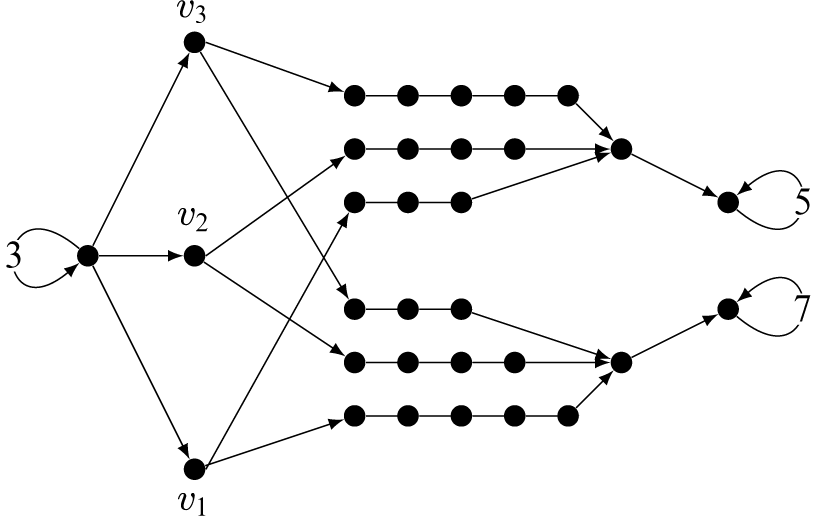
Figure 1 Part of the graph $F(\mathcal {A})$
coding that
$F(\mathcal {A})$
coding that $\mathcal {A}\not \models R_3(3,2,1)$
and
$\mathcal {A}\not \models R_3(3,2,1)$
and $\mathcal {A}\models R_3(1,2,3)$
.
$\mathcal {A}\models R_3(1,2,3)$
.
Let us fix the some notation for the following proofs. Given a structure $\mathcal {A}$
and
$\mathcal {A}$
and $\bar a\in A^{<\omega }$
we let
$\bar a\in A^{<\omega }$
we let $\langle \bar a\rangle ^{\mathcal {A}}$
be the substructure of
$\langle \bar a\rangle ^{\mathcal {A}}$
be the substructure of $\mathcal {A}$
generated by
$\mathcal {A}$
generated by $\bar a$
.
$\bar a$
.
Lemma 3.3. For $\mathcal {A},\mathcal {B}\in \mathfrak {K}$
,
$\mathcal {A},\mathcal {B}\in \mathfrak {K}$
, $\mathcal {A}\mathbin{\preccurlyeq} \mathcal {B}$
if and only if
$\mathcal {A}\mathbin{\preccurlyeq} \mathcal {B}$
if and only if $g(\mathcal {A})\mathbin{\preccurlyeq} g(\mathcal {B})$
.
$g(\mathcal {A})\mathbin{\preccurlyeq} g(\mathcal {B})$
.
Proof. $(\Rightarrow )$
. Assume that
$(\Rightarrow )$
. Assume that $\mathcal {A} \mathbin{\preccurlyeq} \mathcal {B}$
and that
$\mathcal {A} \mathbin{\preccurlyeq} \mathcal {B}$
and that $\mathcal {A}$
is an elementary substructure of
$\mathcal {A}$
is an elementary substructure of $\mathcal {B}$
. We may also assume without loss of generality that
$\mathcal {B}$
. We may also assume without loss of generality that $g(\mathcal {A})\subseteq g(\mathcal {B})$
. We will show that for all
$g(\mathcal {A})\subseteq g(\mathcal {B})$
. We will show that for all $n\in \omega $
and any
$n\in \omega $
and any $\overline {a}\in g(\mathcal {A})^{<\omega }$
Player II has a winning strategy for the n turn Ehrenfeucht–Fraïssé game
$\overline {a}\in g(\mathcal {A})^{<\omega }$
Player II has a winning strategy for the n turn Ehrenfeucht–Fraïssé game $G_n((g({\mathcal {A}}),\overline {a}),(g({\mathcal {B}}),\overline {a}))$
. Assume that n is the least such that Player II has no winning strategy for
$G_n((g({\mathcal {A}}),\overline {a}),(g({\mathcal {B}}),\overline {a}))$
. Assume that n is the least such that Player II has no winning strategy for $G_n((g({\mathcal {A}}),\overline {a}),(g(\mathcal {B}),\overline {a}))$
. Consider the set of partial isomorphisms from
$G_n((g({\mathcal {A}}),\overline {a}),(g(\mathcal {B}),\overline {a}))$
. Consider the set of partial isomorphisms from $(g(\mathcal {A}),\overline {a})$
to
$(g(\mathcal {A}),\overline {a})$
to $(g(\mathcal {B}),\overline {a})$
. This set cannot have the back-and-forth property. In particular, the back-and-forth property fails already if we only consider partial isomorphisms with domain of size
$(g(\mathcal {B}),\overline {a})$
. This set cannot have the back-and-forth property. In particular, the back-and-forth property fails already if we only consider partial isomorphisms with domain of size $n+|\overline {a}|$
. Otherwise there would be a winning strategy for
$n+|\overline {a}|$
. Otherwise there would be a winning strategy for $G_n((g(\mathcal {A}),\overline {a}), (g(\mathcal {B}),\overline {a}))$
. So, either there is
$G_n((g(\mathcal {A}),\overline {a}), (g(\mathcal {B}),\overline {a}))$
. So, either there is $\overline {v} \in g(\mathcal {A})^{n}$
such that for all
$\overline {v} \in g(\mathcal {A})^{n}$
such that for all $\overline {u} \in g(\mathcal {B})^{n}$
,
$\overline {u} \in g(\mathcal {B})^{n}$
, $\langle \overline {a} \overline {v}\rangle ^{g({\mathcal {A}})}\not \cong \langle \overline {a} \overline {u} \rangle ^{g({\mathcal {B}})}$
or there is
$\langle \overline {a} \overline {v}\rangle ^{g({\mathcal {A}})}\not \cong \langle \overline {a} \overline {u} \rangle ^{g({\mathcal {B}})}$
or there is $\overline {u}\in g(\mathcal {B})^{n}$
such that for all
$\overline {u}\in g(\mathcal {B})^{n}$
such that for all $\overline {v} \in g(\mathcal {B})^{n}$
,
$\overline {v} \in g(\mathcal {B})^{n}$
, $\langle \overline {a} \overline {u} \rangle ^{g(\mathcal {B})}\not \cong \langle \overline {a}\overline {v} \rangle ^{g({\mathcal {A}})}$
. We will derive a contradiction assuming the second case. Deriving one from the first case can be done in a similar fashion.
$\langle \overline {a} \overline {u} \rangle ^{g(\mathcal {B})}\not \cong \langle \overline {a}\overline {v} \rangle ^{g({\mathcal {A}})}$
. We will derive a contradiction assuming the second case. Deriving one from the first case can be done in a similar fashion.
Notice that $\overline {a}\overline {u}$
is in a substructure of
$\overline {a}\overline {u}$
is in a substructure of $g({\mathcal {B}})$
coding a finite substructure of
$g({\mathcal {B}})$
coding a finite substructure of $\mathcal {B}$
in a finite part
$\mathcal {B}$
in a finite part $\mathcal {L}_1$
of the language of
$\mathcal {L}_1$
of the language of $\mathcal {B}$
. Extend
$\mathcal {B}$
. Extend $\langle \overline {a} \overline {u}\rangle ^{g({\mathcal {B}})}$
so that it codes such a substructure
$\langle \overline {a} \overline {u}\rangle ^{g({\mathcal {B}})}$
so that it codes such a substructure $\mathcal {B}_1$
of
$\mathcal {B}_1$
of $\mathcal {B}$
. Consider the conjunction
$\mathcal {B}$
. Consider the conjunction $\varphi $
of atomic formulas, or negations thereof, true of
$\varphi $
of atomic formulas, or negations thereof, true of $\mathcal {B}_1$
in
$\mathcal {B}_1$
in $\mathcal {L}_1$
. Let
$\mathcal {L}_1$
. Let $\overline {a}'$
be the elements in
$\overline {a}'$
be the elements in $B_1\cap A$
and
$B_1\cap A$
and $\overline {u}'$
the elements in
$\overline {u}'$
the elements in $B_1\setminus A$
. Then
$B_1\setminus A$
. Then $\mathcal {B} \models \varphi (\overline {a}'\overline {u}')$
and the Tarski–Vaught test gives us elements
$\mathcal {B} \models \varphi (\overline {a}'\overline {u}')$
and the Tarski–Vaught test gives us elements $\overline {v}'$
in
$\overline {v}'$
in $\mathcal {A}$
such that
$\mathcal {A}$
such that $\mathcal {A}\models \varphi (\overline {a}'\overline {v}')$
. It follows that we have a partial isomorphism between
$\mathcal {A}\models \varphi (\overline {a}'\overline {v}')$
. It follows that we have a partial isomorphism between $\langle \overline {a}'\overline {u}'\rangle ^{\mathcal {B}}$
and
$\langle \overline {a}'\overline {u}'\rangle ^{\mathcal {B}}$
and $\langle \overline {a}'\overline {v}'\rangle ^{\mathcal {A}}$
in
$\langle \overline {a}'\overline {v}'\rangle ^{\mathcal {A}}$
in $\mathcal {L}_1$
. This induces an isomorphism between the subgraph coding
$\mathcal {L}_1$
. This induces an isomorphism between the subgraph coding $\mathcal {B}_1$
and the subgraph coding
$\mathcal {B}_1$
and the subgraph coding $\langle \overline {a}'\overline {v}'\rangle ^{\mathcal {A}}$
. But
$\langle \overline {a}'\overline {v}'\rangle ^{\mathcal {A}}$
. But $\langle \overline {a} \overline {u} \rangle ^{g(\mathcal {B})}$
is a subgraph of the graph coding
$\langle \overline {a} \overline {u} \rangle ^{g(\mathcal {B})}$
is a subgraph of the graph coding $\mathcal {B}_1$
and thus it is isomorphic to a substructure
$\mathcal {B}_1$
and thus it is isomorphic to a substructure $\langle \overline {a}\overline {v}\rangle ^{g(\mathcal {A})}$
of the structure coding
$\langle \overline {a}\overline {v}\rangle ^{g(\mathcal {A})}$
of the structure coding $\langle \overline {a}'\overline {v}'\rangle ^{\mathcal {A}}$
, a contradiction.
$\langle \overline {a}'\overline {v}'\rangle ^{\mathcal {A}}$
, a contradiction. $(\Leftarrow )$
. An easy induction on the quantifier depth of formulas in
$(\Leftarrow )$
. An easy induction on the quantifier depth of formulas in $\mathcal {L}$
shows that for every
$\mathcal {L}$
shows that for every $\mathcal {A}\in \mathfrak K$
and
$\mathcal {A}\in \mathfrak K$
and $\mathcal {L}$
-formula
$\mathcal {L}$
-formula $\varphi $
with n-free variables the set
$\varphi $
with n-free variables the set
 $$ \begin{align*}D_\varphi^{\mathcal{A}}=\{ (v_{a_1},\dots, v_{a_n}) : (\mathcal{A},a_1,\dots,a_n) \models \varphi(a_1,\dots,a_n)\}\end{align*} $$
is definable in $g(\mathcal {A})$
. Now, assume that
$g(\mathcal {A})$
. Now, assume that $g(\mathcal {A})\mathbin{\preccurlyeq} g(\mathcal {B})$
and without loss of generality that
$g(\mathcal {A})\mathbin{\preccurlyeq} g(\mathcal {B})$
and without loss of generality that $g(\mathcal {A})$
is an elementary substructure of
$g(\mathcal {A})$
is an elementary substructure of $g(\mathcal {B})$
. Let
$g(\mathcal {B})$
. Let $g_{\mathcal {B}}: \mathcal {B}\mathbin{\rightarrow} g(\mathcal {B})$
be defined by
$g_{\mathcal {B}}: \mathcal {B}\mathbin{\rightarrow} g(\mathcal {B})$
be defined by $g_{\mathcal {B}}: b\mapsto v_b$
. Notice that the map
$g_{\mathcal {B}}: b\mapsto v_b$
. Notice that the map $a\mapsto g_{\mathcal {B}}^{-1}(v_a)$
is an embedding of
$a\mapsto g_{\mathcal {B}}^{-1}(v_a)$
is an embedding of $\mathcal {A}$
in
$\mathcal {A}$
in $\mathcal {B}$
. To see that this embedding is elementary assume that
$\mathcal {B}$
. To see that this embedding is elementary assume that $(\mathcal {A},\overline {a})\models \varphi $
, then
$(\mathcal {A},\overline {a})\models \varphi $
, then $\bar v_{\bar a}\in D_\varphi ^{\mathcal {A}}$
and by elementarity
$\bar v_{\bar a}\in D_\varphi ^{\mathcal {A}}$
and by elementarity $\bar v_{\bar a}\in D_\varphi ^{\mathcal {B}}$
. So,
$\bar v_{\bar a}\in D_\varphi ^{\mathcal {B}}$
. So, $(\mathcal {B}, g_{\mathcal {B}}^{-1}(\bar v_{\bar a}))\models \varphi (g_{\mathcal {B}}^{-1}(\bar v_{\bar a}))$
.⊣
$(\mathcal {B}, g_{\mathcal {B}}^{-1}(\bar v_{\bar a}))\models \varphi (g_{\mathcal {B}}^{-1}(\bar v_{\bar a}))$
.⊣
Concatenating the reductions f and g and from the fact that $\mathbin{\hookrightarrow}_{\mathfrak {G}}$
,
$\mathbin{\hookrightarrow}_{\mathfrak {G}}$
, $\approx _{\mathfrak {G}}$
are complete
$\approx _{\mathfrak {G}}$
are complete $\boldsymbol {\Sigma }^1_1$
quasi-orders, respectively equivalence relations, we obtain Theorem 1.1.
$\boldsymbol {\Sigma }^1_1$
quasi-orders, respectively equivalence relations, we obtain Theorem 1.1.
To prove Theorem 1.2 notice that f and g are computable. Thus there is a Turing operator $\Phi $
such that
$\Phi $
such that $\Phi =g\circ f$
. We can find a Turing machine
$\Phi =g\circ f$
. We can find a Turing machine $\varphi _i$
such that
$\varphi _i$
such that $\varphi _i(j,k)=\Phi ^{\mathcal {A}_j}(k)$
for all
$\varphi _i(j,k)=\Phi ^{\mathcal {A}_j}(k)$
for all $k\in \omega $
if
$k\in \omega $
if $\mathcal {A}_j$
is a total computable structure. Using the s-m-n theorem we can then get a computable function
$\mathcal {A}_j$
is a total computable structure. Using the s-m-n theorem we can then get a computable function $j\mapsto u(i,j)$
where
$j\mapsto u(i,j)$
where $u(i,j)$
is an index for
$u(i,j)$
is an index for $\Phi ^{\mathcal {A}_j}$
. Thus
$\Phi ^{\mathcal {A}_j}$
. Thus $\mathbin{\hookrightarrow}_{\mathfrak {G}}$
is computably reducible to
$\mathbin{\hookrightarrow}_{\mathfrak {G}}$
is computably reducible to $\mathbin{\preccurlyeq}_{\mathfrak {G}}$
as a quasi-order on
$\mathbin{\preccurlyeq}_{\mathfrak {G}}$
as a quasi-order on $\omega $
. Fokina and Friedman [Reference Fokina and Friedman6] showed that
$\omega $
. Fokina and Friedman [Reference Fokina and Friedman6] showed that $\mathbin{\hookrightarrow}_{\mathfrak {G}}$
is
$\mathbin{\hookrightarrow}_{\mathfrak {G}}$
is $\Sigma _1^1$
complete. Thus,
$\Sigma _1^1$
complete. Thus, $\mathbin{\preccurlyeq}_{\mathfrak {G}}$
is also
$\mathbin{\preccurlyeq}_{\mathfrak {G}}$
is also $\Sigma ^1_1$
complete and Theorem 1.2 follows.
$\Sigma ^1_1$
complete and Theorem 1.2 follows.
4 Degree spectra
In this section we finish the proof of Theorem 1.3. As noticed before the two reductions $f: \mathfrak {G}\mathbin{\rightarrow} \mathfrak {C}$
and
$f: \mathfrak {G}\mathbin{\rightarrow} \mathfrak {C}$
and $g:\mathfrak {C}\mathbin{\rightarrow} \mathfrak {G}$
are computable. We will see that the two functions induce an even stronger notion of reduction that allows us to relate the degree spectra realized by
$g:\mathfrak {C}\mathbin{\rightarrow} \mathfrak {G}$
are computable. We will see that the two functions induce an even stronger notion of reduction that allows us to relate the degree spectra realized by $\approx _{\mathfrak {G}}$
and
$\approx _{\mathfrak {G}}$
and $\approxeq _{\mathfrak {G}}$
.
$\approxeq _{\mathfrak {G}}$
.
Definition 4.1 (cf. [Reference Harrison-Trainor, Melnikov, Miller and Montalbán13, Reference Miller, Poonen, Schoutens and Shlapentokh17]).
Let $\mathfrak {C}$
and
$\mathfrak {C}$
and $\mathfrak {D}$
be categories. A computable functor between
$\mathfrak {D}$
be categories. A computable functor between $\mathfrak {C}$
and
$\mathfrak {C}$
and $\mathfrak {D}$
is a pair of computable operators
$\mathfrak {D}$
is a pair of computable operators $(\Phi ,\Phi _*)$
such that
$(\Phi ,\Phi _*)$
such that
-
(1) for all
$\mathcal {A}\in \mathfrak {C}_1$
,
$F(\mathcal {A})=\Phi ^{\mathcal {A}}$
, and -
(2) for all
$f:\mathcal {A}\mathbin{\rightarrow} \mathcal {B}\in \mathfrak {C}_2$
,
$F(f)=\Phi _*^{\mathcal {A}\oplus f\oplus \mathcal {B}}$
.


Computable functors preserve many computability theoretic properties. One example are degree spectra: Recall that for $X,Y\subseteq \mathcal P(\omega )$
, X is Medvedev reducible to Y,
$X,Y\subseteq \mathcal P(\omega )$
, X is Medvedev reducible to Y, $X\leq _s Y$
, if there is a Turing operator
$X\leq _s Y$
, if there is a Turing operator $\Phi $
such that for all
$\Phi $
such that for all $y\in Y$
, there is
$y\in Y$
, there is $x\in X$
such that
$x\in X$
such that $\Phi ^y=x$
. We have in particular that if
$\Phi ^y=x$
. We have in particular that if $F:(\mathfrak {C},{\leadsto }_1)\mathbin{\rightarrow} (\mathfrak {D}, {\leadsto }_2)$
is a computable functor, and
$F:(\mathfrak {C},{\leadsto }_1)\mathbin{\rightarrow} (\mathfrak {D}, {\leadsto }_2)$
is a computable functor, and $\sim _i$
is the equivalence relation given by
$\sim _i$
is the equivalence relation given by
 $$ \begin{align*} \mathcal{A}\sim_i\mathcal{B} \Leftrightarrow \mathcal{A}\mathbin{{\leadsto}_i} \mathcal{B} \land \mathcal{B} \mathbin{{\leadsto}_i} \mathcal{A},\end{align*} $$
then for all $\mathcal {A}\in \mathfrak {C}$
,
$\mathcal {A}\in \mathfrak {C}$
, $\textit{DgSp}_{\sim _1}(F(\mathcal {A}))\leq _s \textit{DgSp}_{\sim _2}(\mathcal {A}).$
It is an easy exercise to see that $g\circ f$
induces a computable functor
$g\circ f$
induces a computable functor $H:(\mathfrak {G},\mathbin{\hookrightarrow})\mathbin{\rightarrow} (\mathfrak {G},\mathbin{\preccurlyeq})$
and thus for all
$H:(\mathfrak {G},\mathbin{\hookrightarrow})\mathbin{\rightarrow} (\mathfrak {G},\mathbin{\preccurlyeq})$
and thus for all $\mathcal {G}\in \mathfrak {G}$
,
$\mathcal {G}\in \mathfrak {G}$
, $\textit{DgSp}_\approx (H(\mathcal {G}))\leq _s \textit{DgSp}_\approxeq (\mathcal {G})$
.
$\textit{DgSp}_\approx (H(\mathcal {G}))\leq _s \textit{DgSp}_\approxeq (\mathcal {G})$
.
To get that every degree spectrum realized in $\mathfrak {C}$
is also realized in
$\mathfrak {C}$
is also realized in $\mathfrak {D}$
we need a stronger notion of reducibility. To define this we need an effectivization of the category theoretic notion of a natural isomorphism between functors.
$\mathfrak {D}$
we need a stronger notion of reducibility. To define this we need an effectivization of the category theoretic notion of a natural isomorphism between functors.
Definition 4.2 [Reference Harrison-Trainor, Melnikov, Miller and Montalbán13].
A functor $F:\mathfrak {C}\mathbin{\rightarrow} \mathfrak {D}$
is effectively isomorphic to
$F:\mathfrak {C}\mathbin{\rightarrow} \mathfrak {D}$
is effectively isomorphic to $G:\mathfrak {C}\mathbin{\rightarrow} \mathfrak {D}$
if there is a Turing operator
$G:\mathfrak {C}\mathbin{\rightarrow} \mathfrak {D}$
if there is a Turing operator $\Lambda $
such that for every
$\Lambda $
such that for every $\mathcal {A}\in \mathfrak {C}$
,
$\mathcal {A}\in \mathfrak {C}$
, $\Lambda ^{\mathcal {A}}$
is an isomorphism from
$\Lambda ^{\mathcal {A}}$
is an isomorphism from $F(\mathcal {A})$
to
$F(\mathcal {A})$
to $G(\mathcal {A})$
, and the following diagram commutes for all
$G(\mathcal {A})$
, and the following diagram commutes for all $\mathcal {A},\mathcal {B}\in \mathfrak {C}_1$
and every
$\mathcal {A},\mathcal {B}\in \mathfrak {C}_1$
and every $\gamma :\mathcal {A}\mathbin{\rightarrow} \mathcal {B}\in \mathfrak {C}_2$
.
$\gamma :\mathcal {A}\mathbin{\rightarrow} \mathcal {B}\in \mathfrak {C}_2$
.

Definition 4.3 (cf. [Reference Harrison-Trainor, Melnikov, Miller and Montalbán13]).
We say that $(\mathfrak {C},{\leadsto }_1)$
is CBF-reducible to
$(\mathfrak {C},{\leadsto }_1)$
is CBF-reducible to $(\mathfrak {D},{\leadsto }_2)$
,
$(\mathfrak {D},{\leadsto }_2)$
, $(\mathfrak {C},{\leadsto }_1)\leq _{CBF}(\mathfrak {D},{\leadsto }_2)$
if
$(\mathfrak {C},{\leadsto }_1)\leq _{CBF}(\mathfrak {D},{\leadsto }_2)$
if
-
(1) there is a computable functor
$F:\mathfrak {C} \mathbin{\rightarrow} \mathfrak {D}$
and a computable functor
$G:\mathfrak {D} \supseteq \hat {\mathfrak {D}}\mathbin{\rightarrow} \mathfrak {C}$
where
$\hat {\mathfrak {D}}$
is the
$\sim _2$
-closure of
$F(\mathfrak {C} )$
, -
(2)
$F\circ G$
is effectively isomorphic to
$Id_{\hat {\mathfrak {D}}}$
,
$G\circ F$
is effectively isomorphic to
$Id_{\mathfrak {C}}$
, and -
(3) if
$\Lambda _{\mathfrak {C}}$
,
$\Lambda _{\mathfrak {D}}$
are the operators witnessing the effective isomorphism between
$G\circ F$
and
$Id_{\mathfrak {C}}$
, respectively,
$F\circ G$
and
$Id_{\hat {\mathfrak {D}}}$
, then for every
$\mathcal {A}\in \mathfrak {C}$
,
$F(\Lambda _{\mathfrak {C}}^{\mathcal {A}})=\Lambda _{\mathfrak {D}}^{F(\mathcal {A})}:F(\mathcal {A}) \mathbin{\rightarrow} F(G(F(\mathcal {A})))$
and every
$\mathcal {B}\in \hat {\mathfrak {D}}$
,
$G(\Lambda _{\mathfrak {D}}^{\mathcal {B}})=\Lambda _{\mathfrak {C}}^{G(\mathcal {B})}:G(\mathcal {B})\mathbin{\rightarrow} G(F(G(\mathcal {B})))$
.


Consider two structures $\mathcal {A}$
and
$\mathcal {A}$
and $\mathcal {B}$
and a morphism
$\mathcal {B}$
and a morphism $f:\mathcal {A}\cong \mathcal {B}$
. Then, clearly
$f:\mathcal {A}\cong \mathcal {B}$
. Then, clearly $\mathcal {A}\leq _T \mathcal {B}\oplus f$
; after all, we have that
$\mathcal {A}\leq _T \mathcal {B}\oplus f$
; after all, we have that $R^{\mathcal {A}}(a_1,\dots , a_n)$
if and only if
$R^{\mathcal {A}}(a_1,\dots , a_n)$
if and only if $R^{\mathcal {B}}(f(a_1),\dots , f(a_n))$
. The following definition generalizes this observation.
$R^{\mathcal {B}}(f(a_1),\dots , f(a_n))$
. The following definition generalizes this observation.
Definition 4.4. A category $\mathfrak {C}$
is degree invariant if for every
$\mathfrak {C}$
is degree invariant if for every $\mathcal {A},\mathcal {B}\in \mathfrak {C}_1$
and every
$\mathcal {A},\mathcal {B}\in \mathfrak {C}_1$
and every $f:\mathcal {A}\mathbin{\rightarrow}\mathcal {B}\in \mathfrak {C}_2$
,
$f:\mathcal {A}\mathbin{\rightarrow}\mathcal {B}\in \mathfrak {C}_2$
, $f\equiv _T f^{-1}$
and
$f\equiv _T f^{-1}$
and $\mathcal {A}\leq _T \mathcal {B}\oplus f$
.
$\mathcal {A}\leq _T \mathcal {B}\oplus f$
.
Proposition 4.5. If $\mathfrak {C}$
and
$\mathfrak {C}$
and $\mathfrak {D}$
are degree invariant and
$\mathfrak {D}$
are degree invariant and $\mathfrak {C}\leq _{CBF} \mathfrak {D}$
, then every set realized as a
$\mathfrak {C}\leq _{CBF} \mathfrak {D}$
, then every set realized as a $\sim _1$
-spectrum in
$\sim _1$
-spectrum in $\mathfrak {C}$
is realized as a
$\mathfrak {C}$
is realized as a $\sim _2$
-spectrum in
$\sim _2$
-spectrum in $\mathfrak {D}$
.
$\mathfrak {D}$
.
Proof. Say $F:\mathfrak {C} \mathbin{\rightarrow} \mathfrak {D}$
and
$F:\mathfrak {C} \mathbin{\rightarrow} \mathfrak {D}$
and $G:\mathfrak {D}\mathbin{\rightarrow} \mathfrak {C}$
witness that
$G:\mathfrak {D}\mathbin{\rightarrow} \mathfrak {C}$
witness that $\mathfrak {C}\leq _{CBF}\mathfrak {D}$
. Fix
$\mathfrak {C}\leq _{CBF}\mathfrak {D}$
. Fix $\mathcal {A}\in \mathfrak {C}$
and let
$\mathcal {A}\in \mathfrak {C}$
and let $\Lambda $
be the Turing operator witnessing that
$\Lambda $
be the Turing operator witnessing that $G\circ F$
is effectively isomorphic to the identity functor on
$G\circ F$
is effectively isomorphic to the identity functor on $\mathfrak {C}$
. Then, for
$\mathfrak {C}$
. Then, for $\hat {\mathcal {A}}\sim _1\mathcal {A}$
,
$\hat {\mathcal {A}}\sim _1\mathcal {A}$
, $\hat {\mathcal {A}}\geq _T F(\hat {\mathcal {A}})\geq _T G(F(\hat {\mathcal {A}}))$
and by degree invariance
$\hat {\mathcal {A}}\geq _T F(\hat {\mathcal {A}})\geq _T G(F(\hat {\mathcal {A}}))$
and by degree invariance $\hat {\mathcal {A}}\leq _T \Lambda ^{\mathcal {A}}\oplus G(F(\hat {\mathcal {A}}))\equiv _T G(F(\hat {\mathcal {A}}))\leq _T F(\hat {\mathcal {A}})$
. Thus,
$\hat {\mathcal {A}}\leq _T \Lambda ^{\mathcal {A}}\oplus G(F(\hat {\mathcal {A}}))\equiv _T G(F(\hat {\mathcal {A}}))\leq _T F(\hat {\mathcal {A}})$
. Thus, $\textit{DgSp}_{\sim _1}(\mathcal {A})\subseteq \textit{DgSp}_{\sim _2}(F(\hat {\mathcal {A}}))$
. The proof that
$\textit{DgSp}_{\sim _1}(\mathcal {A})\subseteq \textit{DgSp}_{\sim _2}(F(\hat {\mathcal {A}}))$
. The proof that $\textit{DgSp}_{\sim _1}(\mathcal {A})\supseteq \textit{DgSp}_{\sim _2}(F(\hat {\mathcal {A}}))$
is similar. So, if X is a
$\textit{DgSp}_{\sim _1}(\mathcal {A})\supseteq \textit{DgSp}_{\sim _2}(F(\hat {\mathcal {A}}))$
is similar. So, if X is a $\sim _1$
spectrum realized by
$\sim _1$
spectrum realized by $\mathcal {A}$
in
$\mathcal {A}$
in $\mathfrak {C}$
, then it is realized as a
$\mathfrak {C}$
, then it is realized as a $\sim _2$
spectrum in
$\sim _2$
spectrum in $\mathfrak {D}$
.⊣
$\mathfrak {D}$
.⊣
Notice that if $\mathfrak {K}$
is a class of relational structures, then whether
$\mathfrak {K}$
is a class of relational structures, then whether $(\mathfrak {K}, {\leadsto })$
is degree invariant only depends on
$(\mathfrak {K}, {\leadsto })$
is degree invariant only depends on ${\leadsto }$
. Thus we might say that a relation on structures is degree invariant.
${\leadsto }$
. Thus we might say that a relation on structures is degree invariant.
Definition 4.6. A class of structures $\mathfrak {C}$
is CBF-complete with respect to a degree invariant relation
$\mathfrak {C}$
is CBF-complete with respect to a degree invariant relation ${\leadsto }$
, if for every class
${\leadsto }$
, if for every class $\mathfrak {K}$
,
$\mathfrak {K}$
, $(\mathfrak {K}, {\leadsto })\leq _{CBF} (\mathfrak {C},{\leadsto })$
.
$(\mathfrak {K}, {\leadsto })\leq _{CBF} (\mathfrak {C},{\leadsto })$
.
We showed in Section 3.2 that for any class $\mathfrak {K}$
equipped with the elementary embeddability relation there is a computable reduction g from
$\mathfrak {K}$
equipped with the elementary embeddability relation there is a computable reduction g from $(\mathfrak {K},\mathbin{\preccurlyeq})$
to
$(\mathfrak {K},\mathbin{\preccurlyeq})$
to $(\mathfrak {G},\mathbin{\preccurlyeq})$
. We can now show that these reductions induce
$(\mathfrak {G},\mathbin{\preccurlyeq})$
. We can now show that these reductions induce $CBF$
-reductions
$CBF$
-reductions $(\mathfrak {K},\mathbin{\preccurlyeq})\leq _{CBF} (\mathfrak {G}\mathbin{\preccurlyeq})$
and that thus graphs are CBF-complete for elementary embeddability. Verifying the conditions of Definition 4.3 is quite technical, but the core ideas of the proof should not be too difficult.
$(\mathfrak {K},\mathbin{\preccurlyeq})\leq _{CBF} (\mathfrak {G}\mathbin{\preccurlyeq})$
and that thus graphs are CBF-complete for elementary embeddability. Verifying the conditions of Definition 4.3 is quite technical, but the core ideas of the proof should not be too difficult.
Theorem 4.7. The class of graphs is CBF-complete for elementary embeddability.
Proof. Fix a class $\mathfrak {K}$
. It is clear from the construction that g induces a computable functor
$\mathfrak {K}$
. It is clear from the construction that g induces a computable functor $F:(\mathfrak {K},\approxeq )\mathbin{\rightarrow} (\mathfrak {G},\approxeq )$
. We have to show that
$F:(\mathfrak {K},\approxeq )\mathbin{\rightarrow} (\mathfrak {G},\approxeq )$
. We have to show that $F(\mathfrak {K})$
is closed under elementary bi-embeddability, that there is a functor
$F(\mathfrak {K})$
is closed under elementary bi-embeddability, that there is a functor $G:F(\mathfrak {K})\mathbin{\rightarrow} \mathfrak {K}$
such that
$G:F(\mathfrak {K})\mathbin{\rightarrow} \mathfrak {K}$
such that $F\circ G$
and
$F\circ G$
and $G\circ F$
are effectively isomorphic to the identity on
$G\circ F$
are effectively isomorphic to the identity on $\mathfrak {K}$
, respectively,
$\mathfrak {K}$
, respectively, $F(\mathfrak {K})$
and that the witnesses of these effective isomorphisms agree.
$F(\mathfrak {K})$
and that the witnesses of these effective isomorphisms agree.
Let $\mathcal {G}\approxeq F(\mathcal {A})$
for some
$\mathcal {G}\approxeq F(\mathcal {A})$
for some $\mathcal {A}\in \mathfrak {K}$
. We may assume without loss of generality that
$\mathcal {A}\in \mathfrak {K}$
. We may assume without loss of generality that $\mathcal {G}$
is an elementary substructure of
$\mathcal {G}$
is an elementary substructure of $F(\mathcal {A})$
. For every
$F(\mathcal {A})$
. For every $\bar a\in \mathcal {G}^{<\omega }$
,
$\bar a\in \mathcal {G}^{<\omega }$
, $\textit{tp}_{\mathcal {G}}(\bar a)=\textit{tp}_{\mathcal {A}}(\bar a)$
. Thus
$\textit{tp}_{\mathcal {G}}(\bar a)=\textit{tp}_{\mathcal {A}}(\bar a)$
. Thus $\mathcal {G}$
must contain the elements
$\mathcal {G}$
must contain the elements $a,b,c$
of
$a,b,c$
of $F(\mathcal {A})$
with unique
$F(\mathcal {A})$
with unique $3$
-cycles, respectively,
$3$
-cycles, respectively, $5$
-cycles and
$5$
-cycles and $7$
-cycles connected to them. Furthermore, say
$7$
-cycles connected to them. Furthermore, say $\bar a \in \mathcal {G}$
codes elements of A in
$\bar a \in \mathcal {G}$
codes elements of A in $F(\mathcal {A})$
such that
$F(\mathcal {A})$
such that $\mathcal {A}\models R_i(\bar a)$
, then this information must also be coded in
$\mathcal {A}\models R_i(\bar a)$
, then this information must also be coded in $\mathcal {G}$
as it is preserved in the type of
$\mathcal {G}$
as it is preserved in the type of $\bar a$
. We can compute a structure
$\bar a$
. We can compute a structure $G(\mathcal {G})$
as follows. Fix a
$G(\mathcal {G})$
as follows. Fix a $\mathcal {G}$
computable injective enumeration f of the set
$\mathcal {G}$
computable injective enumeration f of the set $\{x: a\rightarrowtail x\}$
. Notice that this can be done uniformly since the set
$\{x: a\rightarrowtail x\}$
. Notice that this can be done uniformly since the set $\{x:a\rightarrowtail x\}$
is uniformly computable in all structures in
$\{x:a\rightarrowtail x\}$
is uniformly computable in all structures in $F(\mathfrak {K})$
. Let the universe of
$F(\mathfrak {K})$
. Let the universe of $G(\mathcal {G})$
be the pull-back along f. Then for all
$G(\mathcal {G})$
be the pull-back along f. Then for all $a_1,\dots , a_i=\bar a \in \omega ^{i}$
,
$a_1,\dots , a_i=\bar a \in \omega ^{i}$
, $G(\mathcal {G})\models R_i(\bar a)$
if for every
$G(\mathcal {G})\models R_i(\bar a)$
if for every $a_j$
,
$a_j$
, $j<i$
, there is a chain of
$j<i$
, there is a chain of $i+j$
connected elements
$i+j$
connected elements $y_1,\dots, y_{i+j}$
with
$y_1,\dots, y_{i+j}$
with $f(a_j)\rightarrowtail y_1$
, all j chains share the same last element y and
$f(a_j)\rightarrowtail y_1$
, all j chains share the same last element y and $y\rightarrowtail b$
. Likewise,
$y\rightarrowtail b$
. Likewise, $G(\mathcal {G})\models \neg R_i(\bar a)$
if there are chains satisfying the above conditions with
$G(\mathcal {G})\models \neg R_i(\bar a)$
if there are chains satisfying the above conditions with $y\rightarrowtail c$
. This finishes the construction of
$y\rightarrowtail c$
. This finishes the construction of $G(\mathcal {G})$
.
$G(\mathcal {G})$
.
Let $\mathcal {G},\hat {\mathcal {G}}\in F(\mathfrak {K})$
and
$\mathcal {G},\hat {\mathcal {G}}\in F(\mathfrak {K})$
and $g:\mathcal {G}\mathbin{\preccurlyeq} \hat { \mathcal {G}}$
. As both graphs are elementary bi-embeddable with images of structures in
$g:\mathcal {G}\mathbin{\preccurlyeq} \hat { \mathcal {G}}$
. As both graphs are elementary bi-embeddable with images of structures in $\mathfrak {K}$
, they have unique vertices a, respectively,
$\mathfrak {K}$
, they have unique vertices a, respectively, $\hat a $
with
$\hat a $
with $3$
-cycles connected to them. Computably in
$3$
-cycles connected to them. Computably in $\mathcal {G}$
and
$\mathcal {G}$
and $\hat {\mathcal {G}}$
find the vertices and enumerate the sets
$\hat {\mathcal {G}}$
find the vertices and enumerate the sets $\{ x: a\rightarrowtail x\}$
, and
$\{ x: a\rightarrowtail x\}$
, and $\{ x: \hat a\rightarrowtail x\}$
using the same procedure as in the construction of
$\{ x: \hat a\rightarrowtail x\}$
using the same procedure as in the construction of $G(\mathcal {G})$
above. Let f, respectively,
$G(\mathcal {G})$
above. Let f, respectively, $\hat f$
be these enumerations. Now let
$\hat f$
be these enumerations. Now let $G(g)=\hat f^{-1}\circ g\circ f$
. By construction
$G(g)=\hat f^{-1}\circ g\circ f$
. By construction $G(g):G(\mathcal {G})\mathbin{\hookrightarrow} G(\hat {\mathcal {G}})$
and
$G(g):G(\mathcal {G})\mathbin{\hookrightarrow} G(\hat {\mathcal {G}})$
and $G(g)$
is uniformly computable in
$G(g)$
is uniformly computable in $\mathcal {G}\oplus g\oplus \hat {\mathcal {G}}$
. To see that
$\mathcal {G}\oplus g\oplus \hat {\mathcal {G}}$
. To see that $G(g)$
is elementary, assume towards a contradiction that it is not. Then there is
$G(g)$
is elementary, assume towards a contradiction that it is not. Then there is $\overline {a}\in G(\mathcal {G})$
and
$\overline {a}\in G(\mathcal {G})$
and $\varphi $
such that
$\varphi $
such that $G(\mathcal {G})\models \varphi (\overline {a})$
but
$G(\mathcal {G})\models \varphi (\overline {a})$
but $G(\hat {\mathcal {G}})\not \models \varphi (G(g)(\overline {a}))$
. Recall that the atomic diagram of the tuple
$G(\hat {\mathcal {G}})\not \models \varphi (G(g)(\overline {a}))$
. Recall that the atomic diagram of the tuple $\overline {a}$
is coded in the type of
$\overline {a}$
is coded in the type of $f(\overline {a})$
in
$f(\overline {a})$
in $\mathcal {G}$
and similarly, the atomic diagram of
$\mathcal {G}$
and similarly, the atomic diagram of $G(g)(\overline {a})$
is coded in the type of
$G(g)(\overline {a})$
is coded in the type of $g(f(\overline {a}))$
in
$g(f(\overline {a}))$
in $\hat { \mathcal {G}}$
. So, g could not be elementary, a contradiction.
$\hat { \mathcal {G}}$
. So, g could not be elementary, a contradiction.
To see that $G\circ F$
and
$G\circ F$
and $F\circ G$
are effectively isomorphic to the identities on
$F\circ G$
are effectively isomorphic to the identities on $\mathfrak {K}$
and
$\mathfrak {K}$
and $F(\mathfrak {K})$
, respectively, first note that
$F(\mathfrak {K})$
, respectively, first note that $G(F(\mathcal {A}))\cong \mathcal {A}$
. There is a canonic isomorphism given by the composition of the maps
$G(F(\mathcal {A}))\cong \mathcal {A}$
. There is a canonic isomorphism given by the composition of the maps $a \mapsto v_a$
and the enumeration f of the set
$a \mapsto v_a$
and the enumeration f of the set $\{x: a\rightarrowtail x\}$
, i.e., the isomorphism is defined by
$\{x: a\rightarrowtail x\}$
, i.e., the isomorphism is defined by $a\mapsto f^{-1}(v_a)$
. It is clearly uniformly computable, say by
$a\mapsto f^{-1}(v_a)$
. It is clearly uniformly computable, say by $\Lambda _{\mathfrak {K}}$
. On the other hand let
$\Lambda _{\mathfrak {K}}$
. On the other hand let $\mathcal {G} \in F(\mathfrak {K})$
, then we can compute an isomorphism between
$\mathcal {G} \in F(\mathfrak {K})$
, then we can compute an isomorphism between $F(G(\mathcal {G}))$
and
$F(G(\mathcal {G}))$
and $\mathcal {G}$
by doing the following. Every
$\mathcal {G}$
by doing the following. Every $v\in G$
either defines a relation
$v\in G$
either defines a relation $R_i$
on some tuple, codes an element, or is used to define
$R_i$
on some tuple, codes an element, or is used to define $a, b, c$
. One can computably determine which of the three cases holds. In the second case simply map v to
$a, b, c$
. One can computably determine which of the three cases holds. In the second case simply map v to $v_{f^{-1}(v)}$
, in the third case one can computably determine whether v is used to define
$v_{f^{-1}(v)}$
, in the third case one can computably determine whether v is used to define $a, b, c$
, and, using F and G, computably find the corresponding element in
$a, b, c$
, and, using F and G, computably find the corresponding element in $F(G(\mathcal {G}))$
. In the first case, we have to find the tuple
$F(G(\mathcal {G}))$
. In the first case, we have to find the tuple $\overline {w}$
such that v is involved in the coding of the relation
$\overline {w}$
such that v is involved in the coding of the relation $R_i$
on
$R_i$
on $\bar w$
. We then map v to the corresponding element in the coding of
$\bar w$
. We then map v to the corresponding element in the coding of $R_i$
on the tuple
$R_i$
on the tuple $v_{f^{-1}(\overline {w})}$
. It is easy to see that one can define a Turing operator
$v_{f^{-1}(\overline {w})}$
. It is easy to see that one can define a Turing operator $\Lambda _{\mathfrak {F}(\mathfrak {K})}$
computing this isomorphism. The Turing operators
$\Lambda _{\mathfrak {F}(\mathfrak {K})}$
computing this isomorphism. The Turing operators $\Lambda _{\mathfrak {F}(\mathfrak {K})}$
and
$\Lambda _{\mathfrak {F}(\mathfrak {K})}$
and $\Lambda _{\mathfrak {K}}$
will witness the effective isomorphism between
$\Lambda _{\mathfrak {K}}$
will witness the effective isomorphism between $F\circ G$
and the identity on
$F\circ G$
and the identity on $F(\mathfrak {K})$
, respectively, the effective isomorphism between
$F(\mathfrak {K})$
, respectively, the effective isomorphism between $G\circ F$
and the identity on
$G\circ F$
and the identity on $\mathfrak {G}$
.
$\mathfrak {G}$
.
It remains to show that the diagrams of Definition 4.2 commute and that for all $\mathcal {A}\in \mathfrak {K}$
and
$\mathcal {A}\in \mathfrak {K}$
and $\mathcal {G}\in F(\mathfrak {K})$
,
$\mathcal {G}\in F(\mathfrak {K})$
, $F(\Lambda _{\mathfrak {K}}^{\mathcal {A}})=\Lambda _{F(\mathfrak {K})}^{F(\mathcal {A})}$
and
$F(\Lambda _{\mathfrak {K}}^{\mathcal {A}})=\Lambda _{F(\mathfrak {K})}^{F(\mathcal {A})}$
and $G(\Lambda _{F(\mathfrak {K})}^{\mathcal {G}})=\Lambda _{\mathfrak {K}}^{G(\mathcal {G})}$
. For the commutation of the diagrams, say first that
$G(\Lambda _{F(\mathfrak {K})}^{\mathcal {G}})=\Lambda _{\mathfrak {K}}^{G(\mathcal {G})}$
. For the commutation of the diagrams, say first that $\mathcal {A},\hat {\mathcal {A}}\in \mathfrak {K}$
with
$\mathcal {A},\hat {\mathcal {A}}\in \mathfrak {K}$
with $\iota : \mathcal {A}\mathbin{\preccurlyeq} \hat { \mathcal {A}}$
. Let
$\iota : \mathcal {A}\mathbin{\preccurlyeq} \hat { \mathcal {A}}$
. Let $h:\mathcal {A}\mathbin{\rightarrow} F(\mathcal {A})$
and
$h:\mathcal {A}\mathbin{\rightarrow} F(\mathcal {A})$
and $\hat h: \hat {\mathcal {A}}\mathbin{\rightarrow} F(\mathcal {A})$
given by
$\hat h: \hat {\mathcal {A}}\mathbin{\rightarrow} F(\mathcal {A})$
given by $h,\hat h:a\mapsto v_a$
. We have not given an explicit definition of
$h,\hat h:a\mapsto v_a$
. We have not given an explicit definition of $F(\iota )$
yet. But notice that
$F(\iota )$
yet. But notice that $F(\iota )$
is uniquely determined by the way it maps the elements
$F(\iota )$
is uniquely determined by the way it maps the elements $v_a$
. In particular, if
$v_a$
. In particular, if $\nu (x)=F(\iota )(x)$
on the elements with
$\nu (x)=F(\iota )(x)$
on the elements with $a\rightarrowtail x$
, then
$a\rightarrowtail x$
, then $\nu =F(\iota )$
. Thus we have that
$\nu =F(\iota )$
. Thus we have that
 $$ \begin{align*} G(F(\iota))=\hat f^{-1}\circ F(\iota)\circ f=\hat f^{-1}\circ \hat h \circ\iota\circ h^{-1}\circ f,\end{align*} $$
and $\Lambda _{\mathfrak {K}}^{\mathcal {A}}=f^{-1}\circ h$
, so
$\Lambda _{\mathfrak {K}}^{\mathcal {A}}=f^{-1}\circ h$
, so
 $$ \begin{align*} \Lambda_{\mathfrak{K}}^{\hat{\mathcal{A}}}\circ \iota=\hat f^{-1} \circ\hat h\circ \iota=G(F(\iota))\circ \Lambda_{\mathfrak{K}}^{\mathcal{A}},\end{align*} $$
and thus $G\circ F$
is effectively isomorphic to
$G\circ F$
is effectively isomorphic to $id_{\mathfrak {K}}$
. Now, say
$id_{\mathfrak {K}}$
. Now, say $\mathcal {G},\hat {\mathcal {G}}\in F(\mathfrak {K})$
with
$\mathcal {G},\hat {\mathcal {G}}\in F(\mathfrak {K})$
with $\eta :\mathcal {G}\mathbin{\preccurlyeq} \hat {\mathcal {G}}$
. First let
$\eta :\mathcal {G}\mathbin{\preccurlyeq} \hat {\mathcal {G}}$
. First let $x\in \mathcal {G}$
with
$x\in \mathcal {G}$
with $a\rightarrowtail x$
. Let h, and
$a\rightarrowtail x$
. Let h, and $\hat h$
be as above, then
$\hat h$
be as above, then $(\Lambda _{F(\mathfrak {K})}^{\hat { \mathcal {G}}}\circ \eta )(x)=(\hat h\circ \hat f^{-1}\circ \eta )(x)$
and
$(\Lambda _{F(\mathfrak {K})}^{\hat { \mathcal {G}}}\circ \eta )(x)=(\hat h\circ \hat f^{-1}\circ \eta )(x)$
and $F(\hat f^{-1}\circ \eta \circ f)=\hat h\circ \hat f^{-1}\circ \eta \circ f\circ h^{-1}$
, so
$F(\hat f^{-1}\circ \eta \circ f)=\hat h\circ \hat f^{-1}\circ \eta \circ f\circ h^{-1}$
, so
 $$ \begin{align*}(F(G(\eta))\circ\Lambda_{F(\mathfrak{K})}^{\mathcal{G}})(x)=(F(\hat f^{-1}\circ \eta\circ f)\circ h\circ f^{-1})(x)=(\hat h\circ \hat f^{-1}\circ \eta)(x).\end{align*} $$
Having established that the diagram commutes on the restricted universes we use the fact that any embedding is determined by these parts of the universes to obtain that $F\circ G$
is effectively isomorphic to
$F\circ G$
is effectively isomorphic to $id_{F(\mathfrak {K})}$
.
$id_{F(\mathfrak {K})}$
.
To verify the last condition in Definition 4.3 let $\mathcal {A}\in \mathfrak {K}$
, then on
$\mathcal {A}\in \mathfrak {K}$
, then on $\{x:x\rightarrowtail a\}$
 $$ \begin{align*} F(\Lambda_{\mathfrak{K}}^{\mathcal{A}})(x)=(\hat h\circ f^{-1}\circ h\circ h^{-1})(x)=(\hat h\circ f^{-1})(x)=\Lambda_{F(\mathfrak{K})}^{F(\mathcal{A})}(x)\end{align*} $$
and as there is a unique extension of this to a mapping $F(\mathcal {A})\mathbin{\rightarrow} F(G(F(\mathcal {A})))$ $F(\Lambda _{\mathfrak {K}}^{\mathcal {A}})=\Lambda _{F(\mathfrak {K})}^{F(\mathcal {A})}$
. At last, let
$F(\Lambda _{\mathfrak {K}}^{\mathcal {A}})=\Lambda _{F(\mathfrak {K})}^{F(\mathcal {A})}$
. At last, let $\mathcal {G}\in F(\mathfrak {K})$
, then
$\mathcal {G}\in F(\mathfrak {K})$
, then
 $$ \begin{align*} G(\Lambda^{\mathcal{G}}_{F(\mathfrak{K})})=\hat f^{-1}\circ h\circ f^{-1}\circ f=\hat f^{-1}\circ h=\Lambda_{\mathfrak{K}}^{G(\mathcal{G})},\end{align*} $$
where f is the enumeration of $\{x:x\rightarrowtail a\}$
in
$\{x:x\rightarrowtail a\}$
in $\mathcal {G}$
and
$\mathcal {G}$
and $\hat f$
the one in
$\hat f$
the one in $G(F(\mathcal {G}))$
.⊣
$G(F(\mathcal {G}))$
.⊣
The following is a direct consequence of Proposition 4.5 and Theorem 4.7.
Corollary 4.8. For every structure $\mathcal {A}$
, there is a graph
$\mathcal {A}$
, there is a graph $\mathcal {G}_{\mathcal {A}}$
such that
$\mathcal {G}_{\mathcal {A}}$
such that
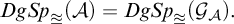 $$ \begin{align*} \textit{DgSp}_\approxeq(\mathcal{A})=\textit{DgSp}_\approxeq(\mathcal{G}_{\mathcal{A}}).\end{align*} $$
Unfortunately, for the reduction from bi-embeddability on graphs to elementary bi-embeddability on $\mathfrak {C}$
given in Section 3.1 we cannot deduce that
$\mathfrak {C}$
given in Section 3.1 we cannot deduce that $(\mathfrak {G},\mathbin{\hookrightarrow})\leq _{CBF} (\mathfrak {C},\mathbin{\preccurlyeq})$
. However, we can still establish a relationship between the degree spectra in these classes. Recall that
$(\mathfrak {G},\mathbin{\hookrightarrow})\leq _{CBF} (\mathfrak {C},\mathbin{\preccurlyeq})$
. However, we can still establish a relationship between the degree spectra in these classes. Recall that $\mathcal {S}_0$
is the substructure of
$\mathcal {S}_0$
is the substructure of $\mathcal {S}$
generated by the constant string of
$\mathcal {S}$
generated by the constant string of $0$
’s and
$0$
’s and $\mathcal {S}_1$
is the substructure generated by the constant string of
$\mathcal {S}_1$
is the substructure generated by the constant string of $1$
’s.
$1$
’s.
Lemma 4.9. Let X be $\Delta ^0_2(Y)$
for some set Y. Then there exist a sequence of structures
$\Delta ^0_2(Y)$
for some set Y. Then there exist a sequence of structures $(\mathcal {C}_i)_{i\in \omega }$
, uniformly computable in Y, such that for all
$(\mathcal {C}_i)_{i\in \omega }$
, uniformly computable in Y, such that for all $i\in \omega $
 $$ \begin{align*} \mathcal{C}_i\cong\begin{cases} \mathcal{S}_0 & \text{if }i\in X,\\ \mathcal{S}_1 &\text{if } i\not\in X.\end{cases}\end{align*} $$
Proof. As X is $\Delta ^0_2$
there is an X-computable two-valued function f such that
$\Delta ^0_2$
there is an X-computable two-valued function f such that
 $$ \begin{align*} \lim_{s{\rightarrow} \infty} f(i,s)=\begin{cases} 0 &\text{if } i\in X,\\ 1&\text{if } i\not\in X.\end{cases}\end{align*} $$
Define a structure $\mathcal {C}$
as follows. Fix an enumeration g of
$\mathcal {C}$
as follows. Fix an enumeration g of $2^{<\omega }$
. At Stage
$2^{<\omega }$
. At Stage $0$
define
$0$
define $\mathcal {C}_0$
to be the partial structure containing one element a on which no relation holds and leave all function symbols undefined. Say we have defined the structure
$\mathcal {C}_0$
to be the partial structure containing one element a on which no relation holds and leave all function symbols undefined. Say we have defined the structure $\mathcal {C}_s$
. At Stage
$\mathcal {C}_s$
. At Stage $s+1$
we look at
$s+1$
we look at $f(i,j)$
for
$f(i,j)$
for $j<s$
and define
$j<s$
and define $\mathcal {C}_{s+1}$
as if a was the finite string with
$\mathcal {C}_{s+1}$
as if a was the finite string with $a(j)=f(j)$
for
$a(j)=f(j)$
for $j<s$
. To be more precise:
$j<s$
. To be more precise:
-
(1) For all k, if
$k\leq s$
and
$|g(k)|\leq s$
then let
$R_{g(k)}(a)$
if and only if
$g(k)\preceq a$
, and if
$F_{g(k)}(a)$
has not been defined yet add a new element and set
$F_{g(k)}(a)$
. -
(2) We may assume by induction that for all elements b in
$\mathcal {C}_{s+1}$
there is
$k\leq s$
such that
$b=F_{g(k)}(a)$
. We set
$R_{g(l)}(b)$
respecting this equation for all
$l\leq s$
.


It is easy to see that this procedure yields a computable sequence of structures $\mathcal {C}_s$
with
$\mathcal {C}_s$
with $\mathcal {C}_s\subseteq \mathcal {C}_{s+1}$
and a computable structure as its limit. We let
$\mathcal {C}_s\subseteq \mathcal {C}_{s+1}$
and a computable structure as its limit. We let $\mathcal {C}$
be this structure.
$\mathcal {C}$
be this structure. $\mathcal {C}$
contains an element a such that
$\mathcal {C}$
contains an element a such that $\mathcal {A}\models R_\sigma (a)$
if and only if
$\mathcal {A}\models R_\sigma (a)$
if and only if $a\preceq f(i,-)$
and all other elements are equal to
$a\preceq f(i,-)$
and all other elements are equal to $F_\tau (a)$
for some
$F_\tau (a)$
for some $\tau \in 2^{<\omega }$
. Thus, in particular if
$\tau \in 2^{<\omega }$
. Thus, in particular if $\lim f(i,s)=0$
, then there is an element representing the constant string of
$\lim f(i,s)=0$
, then there is an element representing the constant string of $0$
’s in
$0$
’s in $\mathcal {A}$
and otherwise there is an element representing the constant string of
$\mathcal {A}$
and otherwise there is an element representing the constant string of $1$
’s in
$1$
’s in $\mathcal {A}$
. Let
$\mathcal {A}$
. Let $\mathcal {C}_i=\mathcal {C}$
, then
$\mathcal {C}_i=\mathcal {C}$
, then $\mathcal {C}_i\cong \mathcal {S}_0$
if and only if
$\mathcal {C}_i\cong \mathcal {S}_0$
if and only if $i\in X$
and
$i\in X$
and $\mathcal {C}_i\cong \mathcal {S}_1$
if and only if
$\mathcal {C}_i\cong \mathcal {S}_1$
if and only if $i\not \in X$
as required.⊣
$i\not \in X$
as required.⊣
We use the usual category theoretic definition of pseudo-inverse. Two functors $F:\mathfrak {C}\mathbin{\rightarrow} \mathfrak {D}$
and
$F:\mathfrak {C}\mathbin{\rightarrow} \mathfrak {D}$
and $G:\mathfrak {D}\mathbin{\rightarrow}\mathfrak {C}$
are pseudo-inverses if
$G:\mathfrak {D}\mathbin{\rightarrow}\mathfrak {C}$
are pseudo-inverses if $F\circ G$
is naturally isomorphic to
$F\circ G$
is naturally isomorphic to $id_{\mathfrak {D}}$
and
$id_{\mathfrak {D}}$
and $G\circ F$
is naturally isomorphic to
$G\circ F$
is naturally isomorphic to $id_{\mathfrak {C}}$
.
$id_{\mathfrak {C}}$
.
Recall that a structure $\mathcal {A}$
is automorphically trivial if there is a finite set
$\mathcal {A}$
is automorphically trivial if there is a finite set $D\subseteq A $
such that every permutation of A that fixes D pointwise is an automorphism. Knight [Reference Louveau and Rosendal16] showed that isomorphism spectra of automorphically trivial structures contain only one Turing degree and that the isomorphism spectra of automorphically non-trivial structures are upwards closed in the Turing degrees. In [Reference Fokina, Rossegger and Mauro7] the authors showed that if
$D\subseteq A $
such that every permutation of A that fixes D pointwise is an automorphism. Knight [Reference Louveau and Rosendal16] showed that isomorphism spectra of automorphically trivial structures contain only one Turing degree and that the isomorphism spectra of automorphically non-trivial structures are upwards closed in the Turing degrees. In [Reference Fokina, Rossegger and Mauro7] the authors showed that if $\mathcal {A}$
is automorphically trivial and
$\mathcal {A}$
is automorphically trivial and $\mathcal {B}\approx \mathcal {A}$
, then
$\mathcal {B}\approx \mathcal {A}$
, then $\mathcal {B}\cong \mathcal {A}$
. Thus, as every bi-embeddability and elementary bi-embeddability spectrum is a union of isomorphism spectra, Knight’s result carries over to this setting.
$\mathcal {B}\cong \mathcal {A}$
. Thus, as every bi-embeddability and elementary bi-embeddability spectrum is a union of isomorphism spectra, Knight’s result carries over to this setting.
Lemma 4.10. For every automorphically non-trivial structure $\mathcal {G}\in \mathfrak {G}$
there is
$\mathcal {G}\in \mathfrak {G}$
there is $\mathcal {A}\in \mathfrak {C}$
such that
$\mathcal {A}\in \mathfrak {C}$
such that
 $$ \begin{align*}\textit{DgSp}_\approxeq(\mathcal{A})=\{X: X'\in \textit{DgSp}_\approx(\mathcal{G})\}.\end{align*} $$
Proof. Recall the reduction from embeddability on graphs to elementary embeddability on $\mathfrak {C}$
given in Section 3.1. It is easy to see that it induces a computable functor
$\mathfrak {C}$
given in Section 3.1. It is easy to see that it induces a computable functor $F: (\mathfrak {G}, \approx )\mathbin{\rightarrow}(\mathfrak {C},\approxeq )$
. We show that the functor has a pseudo-inverse G on the
$F: (\mathfrak {G}, \approx )\mathbin{\rightarrow}(\mathfrak {C},\approxeq )$
. We show that the functor has a pseudo-inverse G on the $\approxeq $
-saturation of
$\approxeq $
-saturation of $F(\mathfrak {G})$
and then use Lemma 4.9 to obtain the lemma. The minimality of the submodels
$F(\mathfrak {G})$
and then use Lemma 4.9 to obtain the lemma. The minimality of the submodels $\mathcal {S}$
used in the construction of F will play a crucial role in the proof.
$\mathcal {S}$
used in the construction of F will play a crucial role in the proof.
Say $\mathcal {B}\approxeq F(\mathcal {G})$
for
$\mathcal {B}\approxeq F(\mathcal {G})$
for $\mathcal {G}\in \mathfrak {G}$
, that
$\mathcal {G}\in \mathfrak {G}$
, that $x,y$
are vertices in
$x,y$
are vertices in $\mathcal {B}$
and
$\mathcal {B}$
and $\mathcal {S}_{(x,y)}$
is the substructure on the elements satisfying
$\mathcal {S}_{(x,y)}$
is the substructure on the elements satisfying $O(x,y,-)$
in the reduct to the language of
$O(x,y,-)$
in the reduct to the language of $\mathcal {S}$
. We have that either
$\mathcal {S}$
. We have that either $\mathcal {S}_{(x,y)}\cong \mathcal {S}_0$
or
$\mathcal {S}_{(x,y)}\cong \mathcal {S}_0$
or $\mathcal {S}_{(x,y)}\cong \mathcal {S}_1$
since it elementary embeds into
$\mathcal {S}_{(x,y)}\cong \mathcal {S}_1$
since it elementary embeds into $\mathcal {S}_{(u,v)}$
for some
$\mathcal {S}_{(u,v)}$
for some $u,v\in F(\mathcal {G})$
and
$u,v\in F(\mathcal {G})$
and $\mathcal {S}_{(u,v)}\cong \mathcal {S}_0$
or
$\mathcal {S}_{(u,v)}\cong \mathcal {S}_0$
or $\mathcal {S}_{(u,v)}\cong \mathcal {S}_1$
by minimality. Thus, we get a graph
$\mathcal {S}_{(u,v)}\cong \mathcal {S}_1$
by minimality. Thus, we get a graph $G(\mathcal {B})$
from
$G(\mathcal {B})$
from $\mathcal {B}$
by defining an edge between two vertex variables
$\mathcal {B}$
by defining an edge between two vertex variables $x,y$
from
$x,y$
from $\mathcal {B}$
if and only if
$\mathcal {B}$
if and only if $\mathcal {S}_{(u,v)}\cong \mathcal {S}_0$
. Clearly every elementary embedding of
$\mathcal {S}_{(u,v)}\cong \mathcal {S}_0$
. Clearly every elementary embedding of $\mathcal {B}$
in
$\mathcal {B}$
in $F(\mathcal {G})$
yields an embedding of
$F(\mathcal {G})$
yields an embedding of $G(\mathcal {B})$
in
$G(\mathcal {B})$
in $\mathcal {G}\cong G(F(\mathcal {G}))$
and the analogous fact is true for every elementary embedding of
$\mathcal {G}\cong G(F(\mathcal {G}))$
and the analogous fact is true for every elementary embedding of $F(\mathcal {G})$
in
$F(\mathcal {G})$
in $\mathcal {B}$
. Likewise, we can argue that
$\mathcal {B}$
. Likewise, we can argue that $F(G(\mathcal {A}))\cong \mathcal {A}$
for every
$F(G(\mathcal {A}))\cong \mathcal {A}$
for every $\mathcal {A}\in F(\mathfrak {G})$
. Thus G and F are pseudo-inverses.
$\mathcal {A}\in F(\mathfrak {G})$
. Thus G and F are pseudo-inverses.
However, notice that G is not effective. Within one jump over the diagram of any $\mathcal {B}\in F(\mathfrak {G})$
we can compute
$\mathcal {B}\in F(\mathfrak {G})$
we can compute $G(\mathcal {B})$
as the isomorphism types of
$G(\mathcal {B})$
as the isomorphism types of $\mathcal {S}_1$
and
$\mathcal {S}_1$
and $\mathcal {S}_0$
are definable by
$\mathcal {S}_0$
are definable by $\Sigma ^c_2$
formulas in
$\Sigma ^c_2$
formulas in $\mathfrak {C}$
. This implies that for all
$\mathfrak {C}$
. This implies that for all $\mathcal {A}\in \mathfrak {G}$
,
$\mathcal {A}\in \mathfrak {G}$
, $F(\mathcal {A})'\geq _T G(F(\mathcal {A}))\cong \mathcal {A}$
. So, in particular,
$F(\mathcal {A})'\geq _T G(F(\mathcal {A}))\cong \mathcal {A}$
. So, in particular,
 $$ \begin{align} \textit{DgSp}_\approxeq(F(\mathcal{A}))\geq_s \{X: X'\in \textit{DgSp}_\approx(G(F(\mathcal{A})))=\textit{DgSp}_\approx(\mathcal{A})\}.\end{align} $$
On the other hand, let $X\in \textit{DgSp}_\approx (\mathcal {A})$
and
$X\in \textit{DgSp}_\approx (\mathcal {A})$
and $\hat {\mathcal {A}}\approx \mathcal {A}$
such that
$\hat {\mathcal {A}}\approx \mathcal {A}$
such that $\hat {\mathcal {A}}\equiv _T X$
. Then by Lemma 4.9 for every Y with
$\hat {\mathcal {A}}\equiv _T X$
. Then by Lemma 4.9 for every Y with $Y'\geq _T X$
, there is
$Y'\geq _T X$
, there is $\mathcal {B}\cong F(\hat {\mathcal {A}})$
with
$\mathcal {B}\cong F(\hat {\mathcal {A}})$
with $\mathcal {B}\equiv _T Y$
. This process is uniform in
$\mathcal {B}\equiv _T Y$
. This process is uniform in $\mathcal {B}$
and Y. Thus
$\mathcal {B}$
and Y. Thus
 $$ \begin{align} \textit{DgSp}_\approxeq(F(\mathcal{A}))\leq_s \{ X: X'\in \textit{DgSp}_\approx(\mathcal{A})\}. \end{align} $$
As both bi-embeddability and elementary bi-embeddability spectra of automorphically non-trivial structures are upwards closed, Equations (1) and (2) imply that
 $$ \begin{align*} \textit{DgSp}_\approxeq(F(\mathcal{A}))=\{ X: X'\in \textit{DgSp}_\approx(\mathcal{A})\}.\end{align*} $$
⊣
Theorem 1.3 follows directly from Lemma 4.10 and Corollary 4.8.
We note that Theorem 1.3 may not be optimal. Using a different proof one might be able to get an even stronger relationship between the spectra realized by bi-embeddability on graphs and elementary bi-embeddability on graphs. We thus ask:
Question 4.11. Is every bi-embeddability spectrum of a graph the elementary bi-embeddability spectrum of a graph and vice versa?
One way to answer this question positively is by showing that if X is an elementary bi-embeddability spectrum then so is $X'=\{ x': x\in X\}$
. This is true for isomorphism spectra and usually shown by considering an appropriate definition for the jump of a structure. However, all known definitions do not preserve elementary embeddability (and not even elementary equivalence). We thus ask:
$X'=\{ x': x\in X\}$
. This is true for isomorphism spectra and usually shown by considering an appropriate definition for the jump of a structure. However, all known definitions do not preserve elementary embeddability (and not even elementary equivalence). We thus ask:
Question 4.12. Let X be the elementary bi-embeddability spectrum of a graph. Is $X'$
the elementary bi-embeddability spectrum of a graph?
$X'$
the elementary bi-embeddability spectrum of a graph?
Question 4.13. Let X be the theory spectrum of a graph. Is $X'$
the theory spectrum of a graph?
$X'$
the theory spectrum of a graph?
Also, while Theorem 4.7 shows that graphs are complete for elementary bi-embeddability spectra, it is unknown whether the same is true for bi-embeddability.
Question 4.14. Is every bi-embeddability spectrum of a structure realized as the bi-embeddability spectrum of a graph?
Acknowledgments
The author thanks David Marker for providing references on minimality. The results in this paper were obtained while the author was a postdoctoral fellow at the Department of Pure Mathematics of the University of Waterloo. The author was partially supported by a Marie Skłodowska-Curie Action under grant agreement No. 101026834—ACOSE.


 Open access