


1 Introduction
The Sun, our nearest star, is a very interesting physical object. One of its mysteries, not yet completely cracked, is the solar corona: very hot
 $(T_{c}\sim 10^{6}~\text{K})$
plasma several thousand kilometres above the visible solar surface (the photosphere). The puzzle is why the corona, while being more distant than the photosphere from the ultimate energy source (which is nuclear fusion reactions in the Sun’s interior), has a temperature much higher than the photosphere (
$(T_{c}\sim 10^{6}~\text{K})$
plasma several thousand kilometres above the visible solar surface (the photosphere). The puzzle is why the corona, while being more distant than the photosphere from the ultimate energy source (which is nuclear fusion reactions in the Sun’s interior), has a temperature much higher than the photosphere (
 $T_{ph}\approx 5800~\text{K}$
). The corona is visible during total solar eclipses as a faint glow around the solar disk when it is covered by the Moon. Although records of eclipses go back millennia, the corona as a separate object has been reported only since the 17th century. Then, during the eclipse of 1869, an unknown green emission line was detected in the coronal spectrum. Since, just a year earlier, another unknown optical line emitted from the Sun had been attributed to a new chemical element named helium, it was tempting to follow suit by introducing another new element, ‘coronium’.
$T_{ph}\approx 5800~\text{K}$
). The corona is visible during total solar eclipses as a faint glow around the solar disk when it is covered by the Moon. Although records of eclipses go back millennia, the corona as a separate object has been reported only since the 17th century. Then, during the eclipse of 1869, an unknown green emission line was detected in the coronal spectrum. Since, just a year earlier, another unknown optical line emitted from the Sun had been attributed to a new chemical element named helium, it was tempting to follow suit by introducing another new element, ‘coronium’.
Although helium was identified in a terrestrial laboratory in 1895, in the case of ‘coronium’ the story turned out to be more complicated. It was not until the 1930s that it was realized that the line under discussion is actually produced by highly ionized iron. This immediately implied that the corona is made of a hot plasma with the temperature exceeding
 $10^{6}~\text{K}$
. Therefore, what is visible around the solar disk during eclipses is mere photospheric light scattered by coronal electrons. The emission of the corona itself falls into the ultraviolet (UV) and soft X-ray bands, and, therefore, can be observed only by space-borne instruments. Thus, state-of-the-art images of the corona, made by the Solar Dynamics Observatory launched in 2010, are available in Main Gallery-SDO/Solar Dynamics Observatory-NASA: sdo.gsfc.nasa.gov/gallery/main. Their distinctive feature is the presence of numerous fine structures, which are a signature of the underlying coronal magnetic field. This field is strong enough to supress the motion of electrons and protons (hydrogen is the main element of the coronal plasma) across magnetic field lines. Indeed, under a typical coronal field strength
$10^{6}~\text{K}$
. Therefore, what is visible around the solar disk during eclipses is mere photospheric light scattered by coronal electrons. The emission of the corona itself falls into the ultraviolet (UV) and soft X-ray bands, and, therefore, can be observed only by space-borne instruments. Thus, state-of-the-art images of the corona, made by the Solar Dynamics Observatory launched in 2010, are available in Main Gallery-SDO/Solar Dynamics Observatory-NASA: sdo.gsfc.nasa.gov/gallery/main. Their distinctive feature is the presence of numerous fine structures, which are a signature of the underlying coronal magnetic field. This field is strong enough to supress the motion of electrons and protons (hydrogen is the main element of the coronal plasma) across magnetic field lines. Indeed, under a typical coronal field strength
 $B_{c}\sim 100~\text{G}$
and plasma density
$B_{c}\sim 100~\text{G}$
and plasma density
 $n_{c}\sim 10^{9}~\text{cm}^{-3}$
(see, e.g. Golub & Pasachoff Reference Golub and Pasachoff2010), the gyrofrequency of protons is
$n_{c}\sim 10^{9}~\text{cm}^{-3}$
(see, e.g. Golub & Pasachoff Reference Golub and Pasachoff2010), the gyrofrequency of protons is
 $\unicode[STIX]{x1D714}_{B}^{(p)}=eB/m_{p}c\sim 10^{6}~\text{s}^{-1}$
, while the collision frequency of thermal protons with energy
$\unicode[STIX]{x1D714}_{B}^{(p)}=eB/m_{p}c\sim 10^{6}~\text{s}^{-1}$
, while the collision frequency of thermal protons with energy
 $E_{p}\sim kT_{c}\sim 10^{2}~\text{eV}$
is approximately
$E_{p}\sim kT_{c}\sim 10^{2}~\text{eV}$
is approximately
 $\unicode[STIX]{x1D708}_{p}\sim 1~\text{s}^{-1}$
. Thus, when
$\unicode[STIX]{x1D708}_{p}\sim 1~\text{s}^{-1}$
. Thus, when
 $\unicode[STIX]{x1D708}_{p}\ll \unicode[STIX]{x1D714}_{B}^{(p)}$
, protons (as well as much lighter plasma electrons) are strongly magnetized, and their gyroradius, which is of the order of
$\unicode[STIX]{x1D708}_{p}\ll \unicode[STIX]{x1D714}_{B}^{(p)}$
, protons (as well as much lighter plasma electrons) are strongly magnetized, and their gyroradius, which is of the order of
 $\unicode[STIX]{x1D70C}_{B}^{(p)}\sim ((\sqrt{kT/m_{p}})/\unicode[STIX]{x1D714}_{B}^{(p)})\sim 10~\text{cm}$
, is negligibly small in the coronal context.
$\unicode[STIX]{x1D70C}_{B}^{(p)}\sim ((\sqrt{kT/m_{p}})/\unicode[STIX]{x1D714}_{B}^{(p)})\sim 10~\text{cm}$
, is negligibly small in the coronal context.
However, guiding charged particles along magnetic field lines is by far not the only role played by the coronal magnetic field. Under the above mentioned coronal parameters, the magnetic energy per unit volume,
 $W_{B}=B_{c}^{2}/8\unicode[STIX]{x03C0}$
, is much larger than the plasma thermal energy
$W_{B}=B_{c}^{2}/8\unicode[STIX]{x03C0}$
, is much larger than the plasma thermal energy
 $W_{T}\sim n_{c}kT_{c}$
. Their ratio is commonly known as a non-dimensional parameter plasma
$W_{T}\sim n_{c}kT_{c}$
. Their ratio is commonly known as a non-dimensional parameter plasma
 $\unicode[STIX]{x1D6FD}$
,
$\unicode[STIX]{x1D6FD}$
,
 $\unicode[STIX]{x1D6FD}\equiv 8\unicode[STIX]{x03C0}nkT/B^{2}$
. In coronal active regions, which look mostly bright in X-ray images of the Sun,
$\unicode[STIX]{x1D6FD}\equiv 8\unicode[STIX]{x03C0}nkT/B^{2}$
. In coronal active regions, which look mostly bright in X-ray images of the Sun,
 $\unicode[STIX]{x1D6FD}\sim 10^{-2}$
. Therefore, the interaction of the solar magnetic field with plasma should be essential for the very existence of the solar corona. Nowadays, it is well known that the Sun is not unique in this respect as X-ray emission associated with coronae is detected from a large number of solar-type stars. However, understanding the mechanism of coronae formation is not only of academic interest. The solar corona is a source of the solar wind, which is the continuous plasma outflow from the Sun that extends far beyond the orbits of the Earth and other planets (see, e.g. Meyer-Vernet Reference Meyer-Vernet2007). Therefore, what is going on in the corona (solar flares, coronal mass ejections, etc.) determines what is presently called ‘Space Weather’ and the resulting terrestrial effects (such as, for example, magnetospheric substorms). Many interesting details about the history of solar coronal studies, as well as the present-day hot topics in this research field, can be found in an excellent book by Golub & Pasachoff (Reference Golub and Pasachoff2010).
$\unicode[STIX]{x1D6FD}\sim 10^{-2}$
. Therefore, the interaction of the solar magnetic field with plasma should be essential for the very existence of the solar corona. Nowadays, it is well known that the Sun is not unique in this respect as X-ray emission associated with coronae is detected from a large number of solar-type stars. However, understanding the mechanism of coronae formation is not only of academic interest. The solar corona is a source of the solar wind, which is the continuous plasma outflow from the Sun that extends far beyond the orbits of the Earth and other planets (see, e.g. Meyer-Vernet Reference Meyer-Vernet2007). Therefore, what is going on in the corona (solar flares, coronal mass ejections, etc.) determines what is presently called ‘Space Weather’ and the resulting terrestrial effects (such as, for example, magnetospheric substorms). Many interesting details about the history of solar coronal studies, as well as the present-day hot topics in this research field, can be found in an excellent book by Golub & Pasachoff (Reference Golub and Pasachoff2010).

Figure 1. Basic elements of the coronal magnetic field. (a) A coronal hole; (b) a coronal loop.
2 Coronal magnetic field and free magnetic energy
Two basic ‘building blocks’ of the coronal magnetic field are schematically drawn in figure 1. The first one, in diagram (a), is the so-called coronal hole. In this case only one end (the footpoint) of a magnetic field line is anchored to the photospheric surface, and the field line extends into the heliosphere. In UV and X-ray images of the Sun, coronal holes look like dim areas on the solar disk because of a low plasma density (charged particles easily escape upward along the magnetic field lines). On the other hand, a bipolar coronal loop, as shown in diagram (b), has both magnetic footpoints connected to the photosphere. Thus, it is a natural plasma trap, and bright regions in the corona are made of such loops. The photospheric surface in figure 1 may be considered a sharp boundary between tenuous low-
 $\unicode[STIX]{x1D6FD}$
coronal plasma and dense sub-photospheric fluid. The energetics of the latter is dominated by the kinetic energy of the convective flow with a velocity of
$\unicode[STIX]{x1D6FD}$
coronal plasma and dense sub-photospheric fluid. The energetics of the latter is dominated by the kinetic energy of the convective flow with a velocity of
 $V_{ph}\sim 1~\text{km}~\text{s}^{-1}$
and a granule size of
$V_{ph}\sim 1~\text{km}~\text{s}^{-1}$
and a granule size of
 $l_{ph}\sim 10^{3}~\text{km}$
. Given this, the photospheric granular turnover time is
$l_{ph}\sim 10^{3}~\text{km}$
. Given this, the photospheric granular turnover time is
 $\unicode[STIX]{x1D70F}_{ph}\sim l_{ph}/V_{ph}\sim 10^{3}~\text{s}$
. This granular flow continuously shuffles footpoints of the coronal magnetic field as shown in figure 1. In the case of coronal holes, these generate magnetohydrodynamic (mainly Alfvén) waves that propagate upward along magnetic field lines, ultimately providing energy input to the solar wind. A very different response comes from the coronal loops. In a low-
$\unicode[STIX]{x1D70F}_{ph}\sim l_{ph}/V_{ph}\sim 10^{3}~\text{s}$
. This granular flow continuously shuffles footpoints of the coronal magnetic field as shown in figure 1. In the case of coronal holes, these generate magnetohydrodynamic (mainly Alfvén) waves that propagate upward along magnetic field lines, ultimately providing energy input to the solar wind. A very different response comes from the coronal loops. In a low-
 $\unicode[STIX]{x1D6FD}$
plasma such as the coronal one, where the dynamics is governed by the magnetic field, perturbations in a system propagate with the Alfvén velocity
$\unicode[STIX]{x1D6FD}$
plasma such as the coronal one, where the dynamics is governed by the magnetic field, perturbations in a system propagate with the Alfvén velocity
 $V_{A}=B/\sqrt{4\unicode[STIX]{x03C0}nm_{p}}$
. With the coronal parameters, one gets
$V_{A}=B/\sqrt{4\unicode[STIX]{x03C0}nm_{p}}$
. With the coronal parameters, one gets
 $V_{A}^{(c)}\sim 10^{3}~\text{km}~\text{s}^{-1}$
, which, for a coronal loop of a typical length
$V_{A}^{(c)}\sim 10^{3}~\text{km}~\text{s}^{-1}$
, which, for a coronal loop of a typical length
 $L_{c}\sim 10^{9}~\text{cm}$
, yields the dynamical time scale of
$L_{c}\sim 10^{9}~\text{cm}$
, yields the dynamical time scale of
 $\unicode[STIX]{x1D70F}_{A}^{(c)}=(L_{c}/V_{A}^{(c)})\sim 10~\text{s}$
. Thus,
$\unicode[STIX]{x1D70F}_{A}^{(c)}=(L_{c}/V_{A}^{(c)})\sim 10~\text{s}$
. Thus,
 $\unicode[STIX]{x1D70F}_{ph}\gg \unicode[STIX]{x1D70F}_{A}^{(c)}$
, which means that such photospheric perturbations are quasistatic. Therefore, the coronal loop remains close to a state of magnetostatic equilibrium at any one time. In a low-
$\unicode[STIX]{x1D70F}_{ph}\gg \unicode[STIX]{x1D70F}_{A}^{(c)}$
, which means that such photospheric perturbations are quasistatic. Therefore, the coronal loop remains close to a state of magnetostatic equilibrium at any one time. In a low-
 $\unicode[STIX]{x1D6FD}$
plasma, where thermal pressure forces are small, this equilibrium requires vanishing magnetic force,
$\unicode[STIX]{x1D6FD}$
plasma, where thermal pressure forces are small, this equilibrium requires vanishing magnetic force,
 $\boldsymbol{F}_{B}=(\boldsymbol{j}\times \boldsymbol{B})/c\approx 0$
, which is the case if electric current
$\boldsymbol{F}_{B}=(\boldsymbol{j}\times \boldsymbol{B})/c\approx 0$
, which is the case if electric current
 $\boldsymbol{j}=c(\unicode[STIX]{x1D735}\times \boldsymbol{B})/4\unicode[STIX]{x03C0}$
flows along magnetic field lines, i.e.
$\boldsymbol{j}=c(\unicode[STIX]{x1D735}\times \boldsymbol{B})/4\unicode[STIX]{x03C0}$
flows along magnetic field lines, i.e.
 $$\begin{eqnarray}(\unicode[STIX]{x1D735}\times \boldsymbol{B})=\unicode[STIX]{x1D6FC}(\boldsymbol{r})\boldsymbol{B}.\end{eqnarray}$$
This equation defines the so-called ‘force-free magnetic field’. Note that since
 $\unicode[STIX]{x1D735}\boldsymbol{\cdot }\boldsymbol{j}=\unicode[STIX]{x1D735}\boldsymbol{\cdot }\boldsymbol{B}=0$
, the function
$\unicode[STIX]{x1D735}\boldsymbol{\cdot }\boldsymbol{j}=\unicode[STIX]{x1D735}\boldsymbol{\cdot }\boldsymbol{B}=0$
, the function
 $\unicode[STIX]{x1D6FC}(\boldsymbol{r})$
in (2.1) should be constant along a magnetic field line but, in a general case may vary from one field line to another. These electric currents are the source of an excess (free) magnetic energy, which is responsible for coronal heating and all other manifestations of coronal activity.
$\unicode[STIX]{x1D6FC}(\boldsymbol{r})$
in (2.1) should be constant along a magnetic field line but, in a general case may vary from one field line to another. These electric currents are the source of an excess (free) magnetic energy, which is responsible for coronal heating and all other manifestations of coronal activity.
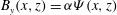
To put the issue of the free magnetic energy on a firm quantitative footing, consider a planar magnetic field shown in figure 2(a). This is clearly a non-potential field, which is evident from the presence of closed magnetic field lines (hence,
 $\oint B\cdot \text{d}l\neq 0\Rightarrow \unicode[STIX]{x1D735}\times \boldsymbol{B}\neq 0\Rightarrow \boldsymbol{j}\neq 0$
). In fact, this is a superposition of the potential X-point magnetic configuration (see figure 2
b) generated by some remote electric currents and the azimuthal field due to an axial electric current concentrated around the X-point (which transforms it into the magnetic O-point).
$\oint B\cdot \text{d}l\neq 0\Rightarrow \unicode[STIX]{x1D735}\times \boldsymbol{B}\neq 0\Rightarrow \boldsymbol{j}\neq 0$
). In fact, this is a superposition of the potential X-point magnetic configuration (see figure 2
b) generated by some remote electric currents and the azimuthal field due to an axial electric current concentrated around the X-point (which transforms it into the magnetic O-point).

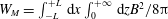
Figure 2. Internal magnetic relaxation. (a) Initial magnetic configuration; (b) relaxed state with a potential magnetic field inside the encircled area. Fine dash-dotted lines indicate ‘separatrices’, which are boundaries between domains of different magnetic field lines connectivity.
Assume now that some process of magnetic relaxation takes place inside the area encircled in figure 2(a). For example, it could be just simple Ohmic dissipation of the central electric current. As far as the exterior of the relaxation circle is concerned, suppose that it is filled with a perfectly conducting and very heavy fluid. Therefore, during the internal magnetic relaxation, this fluid remains immobile because of its strong inertia, so the external magnetic field does not change. What is the minimum of the magnetic energy
 $W_{M}$
inside the circle that can be achieved under such relaxation? Since
$W_{M}$
inside the circle that can be achieved under such relaxation? Since
 $$\begin{eqnarray}W_{M}=\int _{V}\frac{B^{2}}{8\unicode[STIX]{x03C0}}\,\text{d}V,\end{eqnarray}$$
the integrand in (2.2) is always non-negative, and at first glance one may conclude that the sought after minimum corresponds simply to
 $\boldsymbol{B}\equiv 0$
everywhere inside the relaxation volume. However, such a state cannot be reached by the internal magnetic relaxation while the external magnetic field remains unchanged. Indeed, since
$\boldsymbol{B}\equiv 0$
everywhere inside the relaxation volume. However, such a state cannot be reached by the internal magnetic relaxation while the external magnetic field remains unchanged. Indeed, since
 $\unicode[STIX]{x1D735}\boldsymbol{\cdot }\boldsymbol{B}=0$
, the normal component of
$\unicode[STIX]{x1D735}\boldsymbol{\cdot }\boldsymbol{B}=0$
, the normal component of
 $\boldsymbol{B}$
must be continuous at the boundary surface. Therefore, only magnetic fields with a prescribed boundary condition
$\boldsymbol{B}$
must be continuous at the boundary surface. Therefore, only magnetic fields with a prescribed boundary condition
 $B_{n}|_{S}=B_{n}^{(ext)}|_{S}$
are allowed to compete in minimizing the magnetic energy (2.2). (Note that since
$B_{n}|_{S}=B_{n}^{(ext)}|_{S}$
are allowed to compete in minimizing the magnetic energy (2.2). (Note that since
 $\unicode[STIX]{x1D735}\boldsymbol{\cdot }\boldsymbol{B}=0$
, the condition
$\unicode[STIX]{x1D735}\boldsymbol{\cdot }\boldsymbol{B}=0$
, the condition
 $\int _{S}B_{n}^{(ext)}\,\text{d}S=0$
is always satisfied.) The right solution can be guessed with the help of the following qualitative physical consideration. Suppose that inside the relaxation domain there is a finite electric resistivity
$\int _{S}B_{n}^{(ext)}\,\text{d}S=0$
is always satisfied.) The right solution can be guessed with the help of the following qualitative physical consideration. Suppose that inside the relaxation domain there is a finite electric resistivity
 $\unicode[STIX]{x1D702}$
, which results in the Ohmic dissipation power per unit volume being equal to
$\unicode[STIX]{x1D702}$
, which results in the Ohmic dissipation power per unit volume being equal to
 $\unicode[STIX]{x1D702}j^{2}\geqslant 0$
. Since the dissipated energy is tapped from the magnetic energy, the latter will decrease with time until
$\unicode[STIX]{x1D702}j^{2}\geqslant 0$
. Since the dissipated energy is tapped from the magnetic energy, the latter will decrease with time until
 $\boldsymbol{j}=0$
everywhere in the domain, i.e. when the magnetic field there becomes potential. By representing this potential field as
$\boldsymbol{j}=0$
everywhere in the domain, i.e. when the magnetic field there becomes potential. By representing this potential field as
 $\boldsymbol{B}_{p}=\unicode[STIX]{x1D735}\unicode[STIX]{x1D719}$
, and adding the necessary condition
$\boldsymbol{B}_{p}=\unicode[STIX]{x1D735}\unicode[STIX]{x1D719}$
, and adding the necessary condition
 $\unicode[STIX]{x1D735}\boldsymbol{\cdot }\boldsymbol{B}=0$
, the magnetic potential
$\unicode[STIX]{x1D735}\boldsymbol{\cdot }\boldsymbol{B}=0$
, the magnetic potential
 $\unicode[STIX]{x1D719}$
should be a solution of the Laplace equation
$\unicode[STIX]{x1D719}$
should be a solution of the Laplace equation
 $\unicode[STIX]{x1D6FB}^{2}\unicode[STIX]{x1D719}=0$
with the boundary condition
$\unicode[STIX]{x1D6FB}^{2}\unicode[STIX]{x1D719}=0$
with the boundary condition
 $\unicode[STIX]{x2202}\unicode[STIX]{x1D719}/\unicode[STIX]{x2202}n|_{S}=B_{n}^{(ext)}$
. This is the so-called Neumann problem, a classical problem in mathematical physics, and it always has a unique solution (see, e.g. Kannenberg Reference Kannenberg1989 and references therein). Given this, any magnetic field admissible in the domain under consideration can be represented as
$\unicode[STIX]{x2202}\unicode[STIX]{x1D719}/\unicode[STIX]{x2202}n|_{S}=B_{n}^{(ext)}$
. This is the so-called Neumann problem, a classical problem in mathematical physics, and it always has a unique solution (see, e.g. Kannenberg Reference Kannenberg1989 and references therein). Given this, any magnetic field admissible in the domain under consideration can be represented as
 $\boldsymbol{B}=\boldsymbol{B}_{p}+\boldsymbol{b}$
with the boundary condition
$\boldsymbol{B}=\boldsymbol{B}_{p}+\boldsymbol{b}$
with the boundary condition
 $b_{n}|_{S}=0$
. Inserting this expression for
$b_{n}|_{S}=0$
. Inserting this expression for
 $\boldsymbol{B}$
into (2.2) yields
$\boldsymbol{B}$
into (2.2) yields
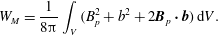 $$\begin{eqnarray}W_{M}=\frac{1}{8\unicode[STIX]{x03C0}}\int _{V}(B_{p}^{2}+b^{2}+2\boldsymbol{B}_{p}\boldsymbol{\cdot }\boldsymbol{b})\,\text{d}V.\end{eqnarray}$$
Since
 $\unicode[STIX]{x1D735}\boldsymbol{\cdot }\boldsymbol{b}=0$
, the last term in the above expression for
$\unicode[STIX]{x1D735}\boldsymbol{\cdot }\boldsymbol{b}=0$
, the last term in the above expression for
 $W_{M}$
can be shown to vanish, as
$W_{M}$
can be shown to vanish, as
 $$\begin{eqnarray}\int _{V}(\boldsymbol{B}_{p}\boldsymbol{\cdot }\boldsymbol{b})\,\text{d}V=\int _{V}(\unicode[STIX]{x1D735}\unicode[STIX]{x1D719}\boldsymbol{\cdot }\boldsymbol{b})\,\text{d}V=\int _{V}\unicode[STIX]{x1D735}(\unicode[STIX]{x1D719}\boldsymbol{b})\,\text{d}V=\int _{S}\unicode[STIX]{x1D719}b_{n}\,\text{d}S=0.\end{eqnarray}$$
Thus, the potential magnetic field corresponds to the state of minimum magnetic energy. Any deviation from this potential field,
 $\boldsymbol{b}$
, which is associated with a non-zero electric current, results in excess magnetic energy
$\boldsymbol{b}$
, which is associated with a non-zero electric current, results in excess magnetic energy
 $\unicode[STIX]{x0394}W_{M}$
given by
$\unicode[STIX]{x0394}W_{M}$
given by
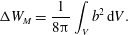 $$\begin{eqnarray}\unicode[STIX]{x0394}W_{M}=\frac{1}{8\unicode[STIX]{x03C0}}\int _{V}b^{2}\,\text{d}V.\end{eqnarray}$$
Returning to the example of figure 2, the respective relaxed state with a potential magnetic field is depicted in figure 2(b). Note that such internal magnetic relaxation is not just a simple elimination of the central electric current. A surface current is induced instead at the boundary surface, which is evident from the discontinuity there of the tangential magnetic field component. Furthermore, there is an apparent change between the initial and the final magnetic configurations. Under the relaxation process, magnetic field lines are allowed to break up and reconnect, resulting in the simplification of the magnetic topology. Such a process, known as ‘magnetic reconnection’, plays an essential role in laboratory and space plasmas. In the context of the solar corona it is briefly discussed in § 4.
3 Energetics of the coronal magnetic arcade
As explained above, force-free magnetic fields, which are defined by (2.1), are at the heart of the solar coronal magnetohydrodynamics. In a real three-dimensional (3-D) solar corona their structure could be quite complicated (Amari et al.
Reference Amari, Aly, Luciani, Boulmezaoud and Mikic1997). Therefore, here we explore a simplified model, where the magnetic field possesses all three spatial components but is invariant with respect to one coordinate (say,
 $y$
). Any such magnetic field can be represented as
$y$
). Any such magnetic field can be represented as
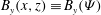
 $$\begin{eqnarray}\boldsymbol{B}(x,z)=[\unicode[STIX]{x1D735}\unicode[STIX]{x1D6F9}(x,z)\times \boldsymbol{e}_{y}]+B_{y}(x,z)\boldsymbol{e}_{y},\end{eqnarray}$$
where
 $\boldsymbol{e}_{y}$
is a unit vector along the
$\boldsymbol{e}_{y}$
is a unit vector along the
 $y$
-axis. This form ensures that
$y$
-axis. This form ensures that
 $\unicode[STIX]{x1D735}\boldsymbol{\cdot }\boldsymbol{B}=0$
. The function
$\unicode[STIX]{x1D735}\boldsymbol{\cdot }\boldsymbol{B}=0$
. The function
 $\unicode[STIX]{x1D6F9}(x,z)$
here is called ‘the poloidal flux function’, while
$\unicode[STIX]{x1D6F9}(x,z)$
here is called ‘the poloidal flux function’, while
 $B_{y}$
is a toroidal field component. This terminology originates from the fusion-oriented research with toroidal laboratory devices. Equation
$B_{y}$
is a toroidal field component. This terminology originates from the fusion-oriented research with toroidal laboratory devices. Equation
 $\unicode[STIX]{x1D6F9}(x,z)=\text{const.}$
determines projections of magnetic field lines on the
$\unicode[STIX]{x1D6F9}(x,z)=\text{const.}$
determines projections of magnetic field lines on the
 $(x,z)$
-plane. Such a projection is defined by the equation
$(x,z)$
-plane. Such a projection is defined by the equation
 $\text{d}x/B_{x}=\text{d}z/B_{z}$
, and since
$\text{d}x/B_{x}=\text{d}z/B_{z}$
, and since
 $B_{x}=-\unicode[STIX]{x2202}\unicode[STIX]{x1D6F9}/\unicode[STIX]{x2202}z,B_{z}=\unicode[STIX]{x2202}\unicode[STIX]{x1D6F9}/\unicode[STIX]{x2202}x$
,
$B_{x}=-\unicode[STIX]{x2202}\unicode[STIX]{x1D6F9}/\unicode[STIX]{x2202}z,B_{z}=\unicode[STIX]{x2202}\unicode[STIX]{x1D6F9}/\unicode[STIX]{x2202}x$
,
 $(\unicode[STIX]{x2202}\unicode[STIX]{x1D6F9}/\unicode[STIX]{x2202}x)\,\text{d}x+(\unicode[STIX]{x2202}\unicode[STIX]{x1D6F9}/\unicode[STIX]{x2202}z)\,\text{d}z=\text{d}\unicode[STIX]{x1D6F9}=0$
along this line. The geometrical meaning of
$(\unicode[STIX]{x2202}\unicode[STIX]{x1D6F9}/\unicode[STIX]{x2202}x)\,\text{d}x+(\unicode[STIX]{x2202}\unicode[STIX]{x1D6F9}/\unicode[STIX]{x2202}z)\,\text{d}z=\text{d}\unicode[STIX]{x1D6F9}=0$
along this line. The geometrical meaning of
 $\unicode[STIX]{x1D6F9}$
becomes evident from calculating the amount of poloidal magnetic flux,
$\unicode[STIX]{x1D6F9}$
becomes evident from calculating the amount of poloidal magnetic flux,
 $\unicode[STIX]{x0394}\unicode[STIX]{x1D6F9}_{p}$
, contained in a 2-D flux tube bounded by two poloidal field lines defined respectively by
$\unicode[STIX]{x0394}\unicode[STIX]{x1D6F9}_{p}$
, contained in a 2-D flux tube bounded by two poloidal field lines defined respectively by
 $\unicode[STIX]{x1D6F9}(x,z)=\unicode[STIX]{x1D6F9}_{1}$
and
$\unicode[STIX]{x1D6F9}(x,z)=\unicode[STIX]{x1D6F9}_{1}$
and
 $\unicode[STIX]{x1D6F9}(x,z)=\unicode[STIX]{x1D6F9}_{2}$
as shown in figure 3.
$\unicode[STIX]{x1D6F9}(x,z)=\unicode[STIX]{x1D6F9}_{2}$
as shown in figure 3.
 $$\begin{eqnarray}\displaystyle \unicode[STIX]{x0394}\unicode[STIX]{x1D6F9}_{p} & = & \displaystyle \int _{1}^{2}\,\text{d}lB_{p}\sin \unicode[STIX]{x1D703}=\boldsymbol{e}_{y}\boldsymbol{\cdot }\int _{1}^{2}(\text{d}\boldsymbol{l}\times \boldsymbol{B}_{p})=\boldsymbol{e}_{y}\boldsymbol{\cdot }\int _{1}^{2}\text{d}\boldsymbol{l}\times (\unicode[STIX]{x1D735}\unicode[STIX]{x1D6F9}\times \boldsymbol{e}_{y})\nonumber\\ \displaystyle & = & \displaystyle -\int _{1}^{2}\text{d}\boldsymbol{l}\boldsymbol{\cdot }\unicode[STIX]{x1D735}\unicode[STIX]{x1D6F9}=\unicode[STIX]{x1D6F9}_{1}-\unicode[STIX]{x1D6F9}_{2}.\end{eqnarray}$$

Figure 3. On the geometrical meaning of the poloidal flux function.
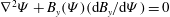
Consider now what condition is required to make the field in (3.1) force free. Thus, according to (3.1),
 $$\begin{eqnarray}(\unicode[STIX]{x1D735}\times \boldsymbol{B})=[\unicode[STIX]{x1D735}B_{y}(x,z)\times \boldsymbol{e}_{y}]-\unicode[STIX]{x1D6FB}^{2}\unicode[STIX]{x1D6F9}(x,z)\boldsymbol{e}_{y}.\end{eqnarray}$$
Since for a force-free field vectors (3.1) and (3.3) are parallel,
 $\unicode[STIX]{x1D735}\unicode[STIX]{x1D6F9}$
should be parallel to
$\unicode[STIX]{x1D735}\unicode[STIX]{x1D6F9}$
should be parallel to
 $\unicode[STIX]{x1D735}\boldsymbol{B}_{y}$
, i.e.
$\unicode[STIX]{x1D735}\boldsymbol{B}_{y}$
, i.e.
 $B_{y}(x,z)\equiv B_{y}(\unicode[STIX]{x1D6F9})$
. This implies that function
$B_{y}(x,z)\equiv B_{y}(\unicode[STIX]{x1D6F9})$
. This implies that function
 $\unicode[STIX]{x1D6FC}(\boldsymbol{r})$
introduced in (2.1) is equal to
$\unicode[STIX]{x1D6FC}(\boldsymbol{r})$
introduced in (2.1) is equal to
 $\unicode[STIX]{x1D6FC}(\boldsymbol{r})=\unicode[STIX]{x1D6FC}(\unicode[STIX]{x1D6F9})=\text{d}B_{y}(\unicode[STIX]{x1D6F9})/\text{d}\unicode[STIX]{x1D6F9}$
. Furthermore, since the ratio of the other components of vectors (3.1) and (3.3) should be equal to the ratio of their poloidal components,
$\unicode[STIX]{x1D6FC}(\boldsymbol{r})=\unicode[STIX]{x1D6FC}(\unicode[STIX]{x1D6F9})=\text{d}B_{y}(\unicode[STIX]{x1D6F9})/\text{d}\unicode[STIX]{x1D6F9}$
. Furthermore, since the ratio of the other components of vectors (3.1) and (3.3) should be equal to the ratio of their poloidal components,
 $-\unicode[STIX]{x1D6FB}^{2}\unicode[STIX]{x1D6F9}=\unicode[STIX]{x1D6FC}B_{y}$
, i.e.
$-\unicode[STIX]{x1D6FB}^{2}\unicode[STIX]{x1D6F9}=\unicode[STIX]{x1D6FC}B_{y}$
, i.e.
 $\unicode[STIX]{x1D6FB}^{2}\unicode[STIX]{x1D6F9}+B_{y}(\unicode[STIX]{x1D6F9})(\text{d}B_{y}/\text{d}\unicode[STIX]{x1D6F9})=0$
. This equation is known in magnetohydrodynamics as the ‘Grad–Shafranov equation’ for a force-free magnetic field. In general, this is a nonlinear equation that reduces to a much simpler linear form when
$\unicode[STIX]{x1D6FB}^{2}\unicode[STIX]{x1D6F9}+B_{y}(\unicode[STIX]{x1D6F9})(\text{d}B_{y}/\text{d}\unicode[STIX]{x1D6F9})=0$
. This equation is known in magnetohydrodynamics as the ‘Grad–Shafranov equation’ for a force-free magnetic field. In general, this is a nonlinear equation that reduces to a much simpler linear form when
 $B_{y}(\unicode[STIX]{x1D6F9})=\unicode[STIX]{x1D6FC}\unicode[STIX]{x1D6F9}$
with
$B_{y}(\unicode[STIX]{x1D6F9})=\unicode[STIX]{x1D6FC}\unicode[STIX]{x1D6F9}$
with
 $\unicode[STIX]{x1D6FC}=\text{const.}$
(the so-called linear force-free magnetic field). In this case the flux function
$\unicode[STIX]{x1D6FC}=\text{const.}$
(the so-called linear force-free magnetic field). In this case the flux function
 $\unicode[STIX]{x1D6F9}$
satisfies the linear equation
$\unicode[STIX]{x1D6F9}$
satisfies the linear equation
 $$\begin{eqnarray}\unicode[STIX]{x1D6FB}^{2}\unicode[STIX]{x1D6F9}+\unicode[STIX]{x1D6FC}^{2}\unicode[STIX]{x1D6F9}=0.\end{eqnarray}$$

Figure 4. Coronal magnetic arcade. (a) Potential magnetic field (
 $\unicode[STIX]{x1D6FC}=0$
); (b) shearing of magnetic field lines (
$\unicode[STIX]{x1D6FC}=0$
); (b) shearing of magnetic field lines (
 $\unicode[STIX]{x1D6FC}\neq 0$
).
$\unicode[STIX]{x1D6FC}\neq 0$
).
Consider now a linear force-free field that does not vary along
 $y$
-axis and corresponds to the flux function
$y$
-axis and corresponds to the flux function
 $$\begin{eqnarray}\unicode[STIX]{x1D6F9}(x,z)=\frac{2B_{0}L}{\unicode[STIX]{x03C0}}\cos \left(\frac{\unicode[STIX]{x03C0}x}{2L}\right)\exp (-\unicode[STIX]{x1D705}z),\quad \unicode[STIX]{x1D705}=\frac{\unicode[STIX]{x03C0}}{2L}\sqrt{1-\frac{4\unicode[STIX]{x1D6FC}^{2}L^{2}}{\unicode[STIX]{x03C0}^{2}}}>0.\end{eqnarray}$$
(It is easy to verify that this
 $\unicode[STIX]{x1D6F9}$
does satisfy (3.4).) In the 2-D domain
$\unicode[STIX]{x1D6F9}$
does satisfy (3.4).) In the 2-D domain
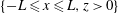 $\{-L\leqslant x\leqslant L,z>0\}$
such a field can be used as a model of the bipolar coronal magnetic arcade located above the photospheric surface
$\{-L\leqslant x\leqslant L,z>0\}$
such a field can be used as a model of the bipolar coronal magnetic arcade located above the photospheric surface
 $z=0$
(see figure 4). When
$z=0$
(see figure 4). When
 $\unicode[STIX]{x1D6FC}=0$
, the field is a potential one with the magnetic field lines lying in the
$\unicode[STIX]{x1D6FC}=0$
, the field is a potential one with the magnetic field lines lying in the
 $(x,z)$
-plane (
$(x,z)$
-plane (
 $B_{y}\equiv 0$
) (figure 4
a). In the non-potential case, when
$B_{y}\equiv 0$
) (figure 4
a). In the non-potential case, when
 $0<\unicode[STIX]{x1D6FC}<\unicode[STIX]{x03C0}/2L$
, the field component
$0<\unicode[STIX]{x1D6FC}<\unicode[STIX]{x03C0}/2L$
, the field component
 $B_{y}(x,z)=\unicode[STIX]{x1D6FC}\unicode[STIX]{x1D6F9}(x,z)$
is present, which makes the magnetic field lines stretch along the
$B_{y}(x,z)=\unicode[STIX]{x1D6FC}\unicode[STIX]{x1D6F9}(x,z)$
is present, which makes the magnetic field lines stretch along the
 $y$
-axis as shown in figure 4(b). Another effect of the non-potentiality of the arcade is its vertical bulging. An increase in
$y$
-axis as shown in figure 4(b). Another effect of the non-potentiality of the arcade is its vertical bulging. An increase in
 $\unicode[STIX]{x1D6FC}$
makes the parameter
$\unicode[STIX]{x1D6FC}$
makes the parameter
 $\unicode[STIX]{x1D705}$
in (3.5) smaller, so the arcade extends further upward. However, note that whatever a magnitude of
$\unicode[STIX]{x1D705}$
in (3.5) smaller, so the arcade extends further upward. However, note that whatever a magnitude of
 $\unicode[STIX]{x1D6FC}$
, the magnetic field defined by (3.5) has the same unchanged normal component at the boundary of the arcade domain. Thus,
$\unicode[STIX]{x1D6FC}$
, the magnetic field defined by (3.5) has the same unchanged normal component at the boundary of the arcade domain. Thus,
 $B_{n}|_{z=0}=B_{z}|_{z=0}=\unicode[STIX]{x2202}\unicode[STIX]{x1D6F9}/\unicode[STIX]{x2202}x|_{z=0}=-B_{0}\sin (\unicode[STIX]{x03C0}x/2L)$
, while
$B_{n}|_{z=0}=B_{z}|_{z=0}=\unicode[STIX]{x2202}\unicode[STIX]{x1D6F9}/\unicode[STIX]{x2202}x|_{z=0}=-B_{0}\sin (\unicode[STIX]{x03C0}x/2L)$
, while
 $B_{n}=0$
at
$B_{n}=0$
at
 $x=\pm L$
and at
$x=\pm L$
and at
 $z\rightarrow +\infty$
. Therefore, as discussed in § 2, the evolution of the magnetic energy in the arcade,
$z\rightarrow +\infty$
. Therefore, as discussed in § 2, the evolution of the magnetic energy in the arcade,
 $W_{M}$
, can be considered independently of its exterior. This energy, calculated per unit length along the
$W_{M}$
, can be considered independently of its exterior. This energy, calculated per unit length along the
 $y$
-axis, is given by the integral
$y$
-axis, is given by the integral
 $W_{M}=\int _{-L}^{+L}\,\text{d}x\int _{0}^{+\infty }\,\text{d}zB^{2}/8\unicode[STIX]{x03C0}$
. Then, according to (3.1) and (3.5), the magnetic field components are equal to
$W_{M}=\int _{-L}^{+L}\,\text{d}x\int _{0}^{+\infty }\,\text{d}zB^{2}/8\unicode[STIX]{x03C0}$
. Then, according to (3.1) and (3.5), the magnetic field components are equal to
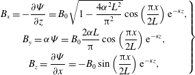 $$\begin{eqnarray}\left.\begin{array}{@{}c@{}}\displaystyle B_{x}=-\frac{\unicode[STIX]{x2202}\unicode[STIX]{x1D6F9}}{\unicode[STIX]{x2202}z}=B_{0}\sqrt{1-\frac{4\unicode[STIX]{x1D6FC}^{2}L^{2}}{\unicode[STIX]{x03C0}^{2}}}\cos \left(\frac{\unicode[STIX]{x03C0}x}{2L}\right)\text{e}^{-\unicode[STIX]{x1D705}z},\\ \displaystyle B_{y}=\unicode[STIX]{x1D6FC}\unicode[STIX]{x1D6F9}=B_{0}\frac{2\unicode[STIX]{x1D6FC}L}{\unicode[STIX]{x03C0}}\cos \left(\frac{\unicode[STIX]{x03C0}x}{2L}\right)\text{e}^{-\unicode[STIX]{x1D705}z},\\ \displaystyle B_{z}=\frac{\unicode[STIX]{x2202}\unicode[STIX]{x1D6F9}}{\unicode[STIX]{x2202}x}=-B_{0}\sin \left(\frac{\unicode[STIX]{x03C0}x}{2L}\right)\text{e}^{-\unicode[STIX]{x1D705}z},\end{array}\right\}\end{eqnarray}$$
and a straightforward integration yields
 $$\begin{eqnarray}W_{M}=\frac{B_{0}^{2}L^{2}}{4\unicode[STIX]{x03C0}^{2}}\left(1-\frac{4\unicode[STIX]{x1D6FC}^{2}L^{2}}{\unicode[STIX]{x03C0}^{2}}\right)^{-1/2}.\end{eqnarray}$$
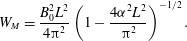
As expected, this magnetic energy is minimal for the potential magnetic field with
 $\unicode[STIX]{x1D6FC}=0$
, so the excess magnetic energy of the arcade is equal to
$\unicode[STIX]{x1D6FC}=0$
, so the excess magnetic energy of the arcade is equal to
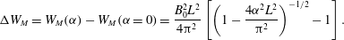 $$\begin{eqnarray}\unicode[STIX]{x0394}W_{M}=W_{M}(\unicode[STIX]{x1D6FC})-W_{M}(\unicode[STIX]{x1D6FC}=0)=\frac{B_{0}^{2}L^{2}}{4\unicode[STIX]{x03C0}^{2}}\left[\left(1-\frac{4\unicode[STIX]{x1D6FC}^{2}L^{2}}{\unicode[STIX]{x03C0}^{2}}\right)^{-1/2}-1\right].\end{eqnarray}$$
The excess magnetic energy is supplied to the corona by photospheric motions (see § 1). Therefore, consider now in more detail the energy balance of this process for the model under discussion. In this case, a signature of the field non-potentiality is its non-zero toroidal component
 $B_{y}$
(and, hence, extension of field lines along the
$B_{y}$
(and, hence, extension of field lines along the
 $y$
-axis). Therefore, the first step is to derive the relation between the non-potentiality parameter
$y$
-axis). Therefore, the first step is to derive the relation between the non-potentiality parameter
 $\unicode[STIX]{x1D6FC}$
and the magnetic footpoints displacement in this direction,
$\unicode[STIX]{x1D6FC}$
and the magnetic footpoints displacement in this direction,
 $\pm y_{0}(x_{0})$
, as shown in figure 4(b). To do so, we define each magnetic field line of the arcade by the parameter
$\pm y_{0}(x_{0})$
, as shown in figure 4(b). To do so, we define each magnetic field line of the arcade by the parameter
 $x_{0}$
, which is the
$x_{0}$
, which is the
 $x$
-coordinate of its footpoints on the photospheric surface
$x$
-coordinate of its footpoints on the photospheric surface
 $z=0$
. In a non-potential field these footpoints are separated in
$z=0$
. In a non-potential field these footpoints are separated in
 $y$
-direction by a distance
$y$
-direction by a distance
 $\unicode[STIX]{x0394}y$
, which can be calculated by using expressions (3.6) for the field components as the following integral along a field line
$\unicode[STIX]{x0394}y$
, which can be calculated by using expressions (3.6) for the field components as the following integral along a field line
 $\unicode[STIX]{x1D6F9}(x,z)=\text{const.}$
:
$\unicode[STIX]{x1D6F9}(x,z)=\text{const.}$
:
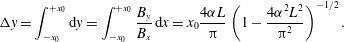 $$\begin{eqnarray}\unicode[STIX]{x0394}y=\int _{-x_{0}}^{+x_{0}}\text{d}y=\int _{-x_{0}}^{+x_{0}}\frac{B_{y}}{B_{x}}\,\text{d}x=x_{0}\frac{4\unicode[STIX]{x1D6FC}L}{\unicode[STIX]{x03C0}}\left(1-\frac{4\unicode[STIX]{x1D6FC}^{2}L^{2}}{\unicode[STIX]{x03C0}^{2}}\right)^{-1/2}.\end{eqnarray}$$
Since
 $$\begin{eqnarray}\unicode[STIX]{x0394}y=2y_{0}(x_{0}),\quad \text{it implies that}~y_{0}(x_{0})=x_{0}\frac{2\unicode[STIX]{x1D6FC}L}{\unicode[STIX]{x03C0}}\left(1-\frac{4\unicode[STIX]{x1D6FC}^{2}L^{2}}{\unicode[STIX]{x03C0}^{2}}\right)^{-1/2}.\end{eqnarray}$$
Assume now that such a displacement is provided by shearing flow
 $V_{y}^{(ph)}(x)$
at the photospheric surface, which forces the magnetic arcade to evolve through a sequence of the force-free equilibria of the form (3.5), with the parameter
$V_{y}^{(ph)}(x)$
at the photospheric surface, which forces the magnetic arcade to evolve through a sequence of the force-free equilibria of the form (3.5), with the parameter
 $\unicode[STIX]{x1D6FC}$
varying with time as some function
$\unicode[STIX]{x1D6FC}$
varying with time as some function
 $\unicode[STIX]{x1D6FC}(t)$
. This requires that
$\unicode[STIX]{x1D6FC}(t)$
. This requires that
 $$\begin{eqnarray}V_{y}^{(ph)}(x_{0})=\frac{\text{d}y_{0}(x_{0})}{\text{d}t}=x_{0}\frac{2L}{\unicode[STIX]{x03C0}}\frac{\text{d}}{\text{d}t}\left[\unicode[STIX]{x1D6FC}\left(1-\frac{4\unicode[STIX]{x1D6FC}^{2}L^{2}}{\unicode[STIX]{x03C0}^{2}}\right)^{-1/2}\right]=x_{0}\frac{2L}{\unicode[STIX]{x03C0}}\left(1-\frac{4\unicode[STIX]{x1D6FC}^{2}L^{2}}{\unicode[STIX]{x03C0}^{2}}\right)^{-3/2}\frac{\text{d}\unicode[STIX]{x1D6FC}}{\text{d}t}.\end{eqnarray}$$
On the other hand, temporal variation of
 $\unicode[STIX]{x1D6FC}$
means that the free magnetic energy (3.8) stored in the arcade is also changing with time. As seen from (3.8), this energy becomes increased for larger
$\unicode[STIX]{x1D6FC}$
means that the free magnetic energy (3.8) stored in the arcade is also changing with time. As seen from (3.8), this energy becomes increased for larger
 $\unicode[STIX]{x1D6FC}$
in the course of the photospheric shearing deformation of the field. Since electric resistivity of the hot coronal plasma is very low (see § 4), the time scale of the magnetic relaxation to a potential ground-energy state is very long. Therefore, during the phase of the magnetic energy storage in the corona, Ohmic dissipation of the magnetic energy is small, so coronal plasma can be considered a perfectly conducting medium with no Ohmic energy losses. Furthermore, under the quasistatic evolution of the arcade, plasma velocity remains highly sub-Alfvénic, so kinetic energy of the plasma flow is small compared to the magnetic energy of the system. Therefore, the energy conservation law requires that the rate of change of the excess magnetic energy (3.8) should be equal to the energy flux supplied to the arcade by the photospheric flow. Since the latter is determined by the Poynting flux
$\unicode[STIX]{x1D6FC}$
in the course of the photospheric shearing deformation of the field. Since electric resistivity of the hot coronal plasma is very low (see § 4), the time scale of the magnetic relaxation to a potential ground-energy state is very long. Therefore, during the phase of the magnetic energy storage in the corona, Ohmic dissipation of the magnetic energy is small, so coronal plasma can be considered a perfectly conducting medium with no Ohmic energy losses. Furthermore, under the quasistatic evolution of the arcade, plasma velocity remains highly sub-Alfvénic, so kinetic energy of the plasma flow is small compared to the magnetic energy of the system. Therefore, the energy conservation law requires that the rate of change of the excess magnetic energy (3.8) should be equal to the energy flux supplied to the arcade by the photospheric flow. Since the latter is determined by the Poynting flux
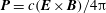 $\boldsymbol{P}=c(\boldsymbol{E}\times \boldsymbol{B})/4\unicode[STIX]{x03C0}$
, the necessary requirement reads
$\boldsymbol{P}=c(\boldsymbol{E}\times \boldsymbol{B})/4\unicode[STIX]{x03C0}$
, the necessary requirement reads
 $$\begin{eqnarray}\frac{\text{d}(\unicode[STIX]{x0394}W_{M})}{\text{d}t}=\left.\int _{-L}^{+L}P_{z}\right|_{z=0}\text{d}x.\end{eqnarray}$$
In a moving perfectly conducting fluid, the electric field is equal to
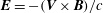 $\boldsymbol{E}=-(\boldsymbol{V}\times \boldsymbol{B})/c$
(see, e.g. Landau, Lifshitz & Pitaevskii Reference Landau, Lifshitz and Pitaevskii1984), and the surface integral in (3.12) can be written as
$\boldsymbol{E}=-(\boldsymbol{V}\times \boldsymbol{B})/c$
(see, e.g. Landau, Lifshitz & Pitaevskii Reference Landau, Lifshitz and Pitaevskii1984), and the surface integral in (3.12) can be written as
 $$\begin{eqnarray}\left.\int _{-L}^{+L}P_{z}\right|_{z=0}\text{d}x=\frac{1}{4\unicode[STIX]{x03C0}}\int _{-L}^{+L}\text{d}x[V_{z}B^{2}-B_{z}(\boldsymbol{V}\boldsymbol{\cdot }\boldsymbol{B})]_{z=0}=-\frac{1}{4\unicode[STIX]{x03C0}}\int _{-L}^{+L}\text{d}xV_{y}^{(ph)}(B_{y}B_{z})_{z=0}.\end{eqnarray}$$
By using expressions (3.6) and (3.11) for the magnetic field and the photospheric velocity, a straightforward calculation of this integral yields
 $$\begin{eqnarray}\int _{L}^{+L}\text{d}xP_{z}(z=0)=\frac{B_{0}^{2}L^{4}}{\unicode[STIX]{x03C0}^{4}}\unicode[STIX]{x1D6FC}\left(1-\frac{4\unicode[STIX]{x1D6FC}^{2}L^{2}}{\unicode[STIX]{x03C0}^{2}}\right)^{-3/2}\frac{\text{d}\unicode[STIX]{x1D6FC}}{\text{d}t},\end{eqnarray}$$
which, according to (3.8), satisfies the energy conservation requirement (3.12). Thus, it completes the demonstration of how mechanical energy of the granular photospheric flow is transformed into the free magnetic energy stored in the solar corona.
4 Energy release: a brief summary
During a fairly strong solar flare, energy of the order of
 $(\unicode[STIX]{x0394}W)_{f}\sim 10^{32}$
erg is released in a matter of tens of minutes (see, e.g. Schrijver Reference Schrijver2009), i.e.
$(\unicode[STIX]{x0394}W)_{f}\sim 10^{32}$
erg is released in a matter of tens of minutes (see, e.g. Schrijver Reference Schrijver2009), i.e.
 $(\unicode[STIX]{x0394}t)_{f}\sim 10^{3}~\text{s}$
. As this energy is tapped from the free magnetic energy stored in the corona, one can estimate what coronal volume
$(\unicode[STIX]{x0394}t)_{f}\sim 10^{3}~\text{s}$
. As this energy is tapped from the free magnetic energy stored in the corona, one can estimate what coronal volume
 $(\unicode[STIX]{x0394}V)_{f}$
should be involved in such an event. Thus, assuming that a respective coronal structure is substantially non-potential, i.e. its non-potential field component
$(\unicode[STIX]{x0394}V)_{f}$
should be involved in such an event. Thus, assuming that a respective coronal structure is substantially non-potential, i.e. its non-potential field component
 $\boldsymbol{b}$
(see § 2) is of the order of
$\boldsymbol{b}$
(see § 2) is of the order of
 $B_{c}\sim 10^{2}~\text{G}$
, one gets from (2.5) that
$B_{c}\sim 10^{2}~\text{G}$
, one gets from (2.5) that
 $b^{2}/8\unicode[STIX]{x03C0}(\unicode[STIX]{x0394}V)_{f}\sim B_{c}^{2}/8\unicode[STIX]{x03C0}(\unicode[STIX]{x0394}V)_{f}\sim (\unicode[STIX]{x0394}W)_{f}$
, which yields
$b^{2}/8\unicode[STIX]{x03C0}(\unicode[STIX]{x0394}V)_{f}\sim B_{c}^{2}/8\unicode[STIX]{x03C0}(\unicode[STIX]{x0394}V)_{f}\sim (\unicode[STIX]{x0394}W)_{f}$
, which yields
 $(\unicode[STIX]{x0394}V)_{f}\sim 3\times 10^{28}~\text{cm}^{3}$
, and, hence, the scale length
$(\unicode[STIX]{x0394}V)_{f}\sim 3\times 10^{28}~\text{cm}^{3}$
, and, hence, the scale length
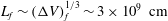 $L_{f}\sim (\unicode[STIX]{x0394}V)_{f}^{1/3}\sim 3\times 10^{9}~\text{cm}$
. It looks quite reasonable since such
$L_{f}\sim (\unicode[STIX]{x0394}V)_{f}^{1/3}\sim 3\times 10^{9}~\text{cm}$
. It looks quite reasonable since such
 $L_{f}$
is comparable to a typical loop length
$L_{f}$
is comparable to a typical loop length
 $L_{c}$
in a coronal active region. There is, however, a striking disparity between the observed flare time
$L_{c}$
in a coronal active region. There is, however, a striking disparity between the observed flare time
 $(\unicode[STIX]{x0394}t)_{f}$
and the time
$(\unicode[STIX]{x0394}t)_{f}$
and the time
 $\unicode[STIX]{x1D70F}_{\unicode[STIX]{x1D702}}$
of the global resistive magnetic energy dissipation in the corona. If one assumes that the non-potential field component
$\unicode[STIX]{x1D70F}_{\unicode[STIX]{x1D702}}$
of the global resistive magnetic energy dissipation in the corona. If one assumes that the non-potential field component
 $\boldsymbol{b}$
varies on a length scale of the order of
$\boldsymbol{b}$
varies on a length scale of the order of
 $L_{c}$
, the electric current in the corona can be estimated as
$L_{c}$
, the electric current in the corona can be estimated as
 $\boldsymbol{j}_{(L_{c})}=c(\unicode[STIX]{x1D735}\times \boldsymbol{b})/4\unicode[STIX]{x03C0}\sim cb/4\unicode[STIX]{x03C0}L_{c}$
. The volumetric power of Ohmic dissipation is equal to
$\boldsymbol{j}_{(L_{c})}=c(\unicode[STIX]{x1D735}\times \boldsymbol{b})/4\unicode[STIX]{x03C0}\sim cb/4\unicode[STIX]{x03C0}L_{c}$
. The volumetric power of Ohmic dissipation is equal to
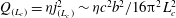 $Q_{(L_{c})}=\unicode[STIX]{x1D702}j_{(L_{c})}^{2}\sim \unicode[STIX]{x1D702}c^{2}b^{2}/16\unicode[STIX]{x03C0}^{2}L_{c}^{2}$
and, hence, it yields the respective dissipation time of
$Q_{(L_{c})}=\unicode[STIX]{x1D702}j_{(L_{c})}^{2}\sim \unicode[STIX]{x1D702}c^{2}b^{2}/16\unicode[STIX]{x03C0}^{2}L_{c}^{2}$
and, hence, it yields the respective dissipation time of
 $$\begin{eqnarray}\unicode[STIX]{x1D70F}_{\unicode[STIX]{x1D702}}\sim \frac{b^{2}/8\unicode[STIX]{x03C0}}{Q}\sim \frac{L_{c}^{2}}{D_{\unicode[STIX]{x1D702}}},\quad \text{where}~D_{\unicode[STIX]{x1D702}}\equiv \frac{\unicode[STIX]{x1D702}c^{2}}{4\unicode[STIX]{x03C0}}\end{eqnarray}$$
is the so called resistive magnetic diffusivity of a medium. In a hot fully ionized plasma this magnetic diffusivity scales as
 $D_{\unicode[STIX]{x1D702}}\propto T^{-3/2}$
, and at the coronal temperature of
$D_{\unicode[STIX]{x1D702}}\propto T^{-3/2}$
, and at the coronal temperature of
 $T_{c}\sim 10^{6}~\text{K}$
it becomes equal to
$T_{c}\sim 10^{6}~\text{K}$
it becomes equal to
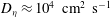 $D_{\unicode[STIX]{x1D702}}\approx 10^{4}~\text{cm}^{2}~\text{s}^{-1}$
. Thus, for
$D_{\unicode[STIX]{x1D702}}\approx 10^{4}~\text{cm}^{2}~\text{s}^{-1}$
. Thus, for
 $L_{c}\sim 10^{9}~\text{cm}$
it yields the global dissipation time
$L_{c}\sim 10^{9}~\text{cm}$
it yields the global dissipation time
 $\unicode[STIX]{x1D70F}_{\unicode[STIX]{x1D702}}\approx 10^{14}~\text{s}$
(i.e.
$\unicode[STIX]{x1D70F}_{\unicode[STIX]{x1D702}}\approx 10^{14}~\text{s}$
(i.e.
 ${\approx}3$
million years!), which is clearly completely irrelevant.
${\approx}3$
million years!), which is clearly completely irrelevant.
It should be noted, however, that such a long time is required for a complete magnetic relaxation to the ground-energy state with a potential magnetic field. Instead, a fraction (typically, a substantial one) of the excess magnetic energy (2.5) can be released much faster via the process of magnetic reconnection (Yamada, Kulsrud & Ji Reference Yamada, Kulsrud and Ji2010). In this case, the electric current is not distributed smoothly throughout the whole relaxation domain (as it was assumed in the estimation of
 $j_{c}$
given above) but is strongly concentrated inside some small regions with a spatial scale
$j_{c}$
given above) but is strongly concentrated inside some small regions with a spatial scale
 $l\ll L_{c}$
. In these regions, called ‘current sheets’, the electric current density
$l\ll L_{c}$
. In these regions, called ‘current sheets’, the electric current density
 $j_{l}$
is much higher than
$j_{l}$
is much higher than
 $j_{L_{c}}$
,
$j_{L_{c}}$
,
 $j_{l}\sim j_{L_{c}}(L_{c}/l)\gg j_{L_{c}}$
. Therefore, the role of even a weak resistivity becomes significantly enhanced inside such current sheets, which results in a much faster breaking up of magnetic field lines. This local effect allows global restructuring of the magnetic field that brings about a partially relaxed state. The latter, being an equilibrium configuration in a low-
$j_{l}\sim j_{L_{c}}(L_{c}/l)\gg j_{L_{c}}$
. Therefore, the role of even a weak resistivity becomes significantly enhanced inside such current sheets, which results in a much faster breaking up of magnetic field lines. This local effect allows global restructuring of the magnetic field that brings about a partially relaxed state. The latter, being an equilibrium configuration in a low-
 $\unicode[STIX]{x1D6FD}$
plasma, should be a force-free magnetic field described by (2.1). Quite remarkably, it turns out that these partially relaxed states correspond to constant-
$\unicode[STIX]{x1D6FD}$
plasma, should be a force-free magnetic field described by (2.1). Quite remarkably, it turns out that these partially relaxed states correspond to constant-
 $\unicode[STIX]{x1D6FC}$
force-free fields for which the function
$\unicode[STIX]{x1D6FC}$
force-free fields for which the function
 $\unicode[STIX]{x1D6FC}(\boldsymbol{r})=\text{const}$
. The reason is associated with a characteristic of the magnetic configuration known as global magnetic helicity
$\unicode[STIX]{x1D6FC}(\boldsymbol{r})=\text{const}$
. The reason is associated with a characteristic of the magnetic configuration known as global magnetic helicity
 $H=\int _{V}\boldsymbol{A}\boldsymbol{\cdot }\boldsymbol{B}\,\text{d}V$
, where
$H=\int _{V}\boldsymbol{A}\boldsymbol{\cdot }\boldsymbol{B}\,\text{d}V$
, where
 $\boldsymbol{A}$
is a vector potential of the magnetic field. This quantity, which is a measure of the twistedness and knottedness of the magnetic field (see, e.g. Pfister & Gekelman Reference Pfister and Gekelman1991 and references therein), is approximately conserved under magnetic reconnection in small current sheets (Taylor Reference Taylor1974, Reference Taylor1986). Therefore, constant-
$\boldsymbol{A}$
is a vector potential of the magnetic field. This quantity, which is a measure of the twistedness and knottedness of the magnetic field (see, e.g. Pfister & Gekelman Reference Pfister and Gekelman1991 and references therein), is approximately conserved under magnetic reconnection in small current sheets (Taylor Reference Taylor1974, Reference Taylor1986). Therefore, constant-
 $\unicode[STIX]{x1D6FC}$
fields represent a minimum of the total magnetic energy under the constraint of a constant magnetic helicity (Woltjer Reference Woltjer1958). Note that complete magnetic relaxation to a potential magnetic configuration, helicity of which is equal to zero, implies destruction of the magnetic helicity.
$\unicode[STIX]{x1D6FC}$
fields represent a minimum of the total magnetic energy under the constraint of a constant magnetic helicity (Woltjer Reference Woltjer1958). Note that complete magnetic relaxation to a potential magnetic configuration, helicity of which is equal to zero, implies destruction of the magnetic helicity.
In the context of magnetic relaxation in the solar corona, a possible role of magnetic helicity and constant-
 $\unicode[STIX]{x1D6FC}$
force-free fields has been first discussed in Norman & Heyvaerts (Reference Norman and Heyvaerts1983). Since small-scale current sheets are likely to form quite readily in the solar corona (Parker Reference Parker1972), magnetic reconnection seems to represent a viable mechanism that underlies solar coronal activity. There is also direct observational evidence of reconfiguration of the magnetic field in the corona, presumably due to magnetic reconnection, during solar flares (Tsuneta Reference Tsuneta1996).
$\unicode[STIX]{x1D6FC}$
force-free fields has been first discussed in Norman & Heyvaerts (Reference Norman and Heyvaerts1983). Since small-scale current sheets are likely to form quite readily in the solar corona (Parker Reference Parker1972), magnetic reconnection seems to represent a viable mechanism that underlies solar coronal activity. There is also direct observational evidence of reconfiguration of the magnetic field in the corona, presumably due to magnetic reconnection, during solar flares (Tsuneta Reference Tsuneta1996).
Consider now the time scale
 $\unicode[STIX]{x1D70F}_{R}$
of the partial magnetic relaxation via the current sheets reconnection. Here it is useful to introduce a non-dimensional parameter called the Lundquist number, which is defined as
$\unicode[STIX]{x1D70F}_{R}$
of the partial magnetic relaxation via the current sheets reconnection. Here it is useful to introduce a non-dimensional parameter called the Lundquist number, which is defined as
 $S\equiv \unicode[STIX]{x1D70F}_{\unicode[STIX]{x1D702}}/\unicode[STIX]{x1D70F}_{A}=LV/D_{\unicode[STIX]{x1D702}}$
. This is typically very large for high-temperature plasma applications in laboratory and space. For example, in fusion-oriented devices,
$S\equiv \unicode[STIX]{x1D70F}_{\unicode[STIX]{x1D702}}/\unicode[STIX]{x1D70F}_{A}=LV/D_{\unicode[STIX]{x1D702}}$
. This is typically very large for high-temperature plasma applications in laboratory and space. For example, in fusion-oriented devices,
 $S\sim 10^{6}$
, while in the solar corona
$S\sim 10^{6}$
, while in the solar corona
 $S_{c}\sim 10^{12}{-}10^{14}$
. Thus, under
$S_{c}\sim 10^{12}{-}10^{14}$
. Thus, under
 $S\gg 1$
, the classical Sweet–Parker model (Parker Reference Parker1957; Sweet Reference Sweet1958) of the current sheet reconnection yields
$S\gg 1$
, the classical Sweet–Parker model (Parker Reference Parker1957; Sweet Reference Sweet1958) of the current sheet reconnection yields
 $\unicode[STIX]{x1D70F}_{R}\sim \unicode[STIX]{x1D70F}_{A}S^{1/2}$
. Although this time is much shorter than the global resistive time
$\unicode[STIX]{x1D70F}_{R}\sim \unicode[STIX]{x1D70F}_{A}S^{1/2}$
. Although this time is much shorter than the global resistive time
 $\unicode[STIX]{x1D70F}_{\unicode[STIX]{x1D702}}=\unicode[STIX]{x1D70F}_{A}S$
that is required for the complete magnetic relaxation, it is still far too long to account for what is actually observed. Moreover, note that the time scale of solar flares, which is
$\unicode[STIX]{x1D70F}_{\unicode[STIX]{x1D702}}=\unicode[STIX]{x1D70F}_{A}S$
that is required for the complete magnetic relaxation, it is still far too long to account for what is actually observed. Moreover, note that the time scale of solar flares, which is
 $(\unicode[STIX]{x0394}t)_{f}\sim 10^{3}~\text{s}$
, is only approximately hundred times longer than the coronal Alfvén transit time
$(\unicode[STIX]{x0394}t)_{f}\sim 10^{3}~\text{s}$
, is only approximately hundred times longer than the coronal Alfvén transit time
 $\unicode[STIX]{x1D70F}_{A}\sim 10~\text{s}$
. Therefore, bearing in mind the extremely large value of the Lundquist number
$\unicode[STIX]{x1D70F}_{A}\sim 10~\text{s}$
. Therefore, bearing in mind the extremely large value of the Lundquist number
 $S_{c}$
, one has to conclude that any realistic theoretical model of solar flares should yield the relaxation time which is virtually independent on a magnitude of the Lundquist number. This issue, called the problem of fast magnetic reconnection, is presently a hot research topic (see, e.g. Loureiro & Uzdensky (Reference Loureiro and Uzdensky2016) for its most recent developments).
$S_{c}$
, one has to conclude that any realistic theoretical model of solar flares should yield the relaxation time which is virtually independent on a magnitude of the Lundquist number. This issue, called the problem of fast magnetic reconnection, is presently a hot research topic (see, e.g. Loureiro & Uzdensky (Reference Loureiro and Uzdensky2016) for its most recent developments).
Acknowledgements
The author is grateful to M. Gordovskyy for his help in preparing the figures for this article, as well as to G. Bendo, I. Browne, and P. Browning for a number of useful comments.


