


1 Introduction
Self-organisation and emergent phenomena in systems with many degrees of freedom and that are far from thermal equilibrium remain a frontier in physics. In fluid dynamics, where turbulence and strong nonlinearities are ubiquitous, the difficulty is amplified because many standard techniques are unavailable.
A striking example of self-organisation is zonal flow, which refers to banded flows alternating in space and quasi-stationary in time. Zonal flow is formed from and coexists with turbulence in the diverse physical contexts of magnetically confined toroidal plasmas (Diamond et al. Reference Diamond, Itoh, Itoh and Hahm2005; Fujisawa Reference Fujisawa2009; Hillesheim et al. Reference Hillesheim, Delabie, Meyer, Maggi, Meneses, Poli and Contributors2016), planetary atmospheres (Vasavada & Showman Reference Vasavada and Showman2005) and possibly astrophysical discs (Johansen, Youdin & Klahr Reference Johansen, Youdin and Klahr2009; Kunz & Lesur Reference Kunz and Lesur2013). Common to each of these physical systems are directions of symmetry, driven turbulent flow and a gradient in the rotation, density, pressure or other background quantity.
In recent years, a quasi-linear approximation has facilitated progress in the fundamental understanding of zonal flows (Farrell & Ioannou Reference Farrell and Ioannou2003, Reference Farrell and Ioannou2007; Marston, Conover & Schneider Reference Marston, Conover and Schneider2008; Srinivasan & Young Reference Srinivasan and Young2012; Bakas & Ioannou Reference Bakas and Ioannou2013; Parker & Krommes Reference Parker and Krommes2013, Reference Parker and Krommes2014; Tobias & Marston Reference Tobias and Marston2013; Constantinou, Farrell & Ioannou Reference Constantinou, Farrell and Ioannou2014; Bakas, Constantinou & Ioannou Reference Bakas, Constantinou and Ioannou2015; Constantinou, Farrell & Ioannou Reference Constantinou, Farrell and Ioannou2016). The quasi-linear approximation involves neglecting the fluctuation self-nonlinearity while retaining the basic nonlinear coupling between mean flows and fluctuations. This truncation eliminates the Kolmogorov cascades and wave–wave interactions, but numerical simulations of quasi-linear dynamics show that fluctuations can still drive the spontaneous formation of zonal flows (Srinivasan & Young Reference Srinivasan and Young2012). Hence, even though many fluid systems are naturally turbulent, turbulence per se is not a critical factor in driving zonal flows, and many aspects of the problem can be qualitatively understood in the simpler quasi-linear setting. This approach has found use beyond zonal flows for understanding generation of other large-scale structures such as the magnetorotational dynamo (Squire & Bhattacharjee Reference Squire and Bhattacharjee2015) and rolls and streaks in wall-bounded shear flow (Farrell & Ioannou Reference Farrell and Ioannou2012). In these quasi-linear models, fluctuations are typically driven by external white noise forcing, an analytically convenient assumption. It should be emphasized that the quasi-linear approximation is a model useful for gaining insight, and one does not expect its quantitative predictions to be correct, particularly when the mean flow is weak.
Because the quasi-linear system couples the fluctuations with the mean field, the equations are stochastically linear, despite being dynamically nonlinear. One can therefore apply an averaging procedure and derive an equation of motion for the covariance without facing the standard closure problem of turbulence in which unknown triple correlations appear.
This averaging leads to a coupled set of equations for the two-point, one-time covariance of the fluctuations and the mean flow (Farrell & Ioannou Reference Farrell and Ioannou2003, Reference Farrell and Ioannou2007; Marston et al. Reference Marston, Conover and Schneider2008; Srinivasan & Young Reference Srinivasan and Young2012). These equations are called CE2, short for second-order cumulant expansion. CE2 offers a set of nonlinear deterministic equations in which rapid fluctuations have been averaged away yet is still equivalent to the quasi-linear dynamics, and is the simplest consistent statistical formulation in which to study inhomogeneous flows.
It is impossible to overstate the importance of CE2 in the context of the quasi-linear model. If statistical inhomogeneity exists in only one dimension, then in a particular limit and with a particular averaging procedure, CE2 describes the exact dynamics of a single realization, not merely the statistics of an ensemble of trajectories (Srinivasan & Young Reference Srinivasan and Young2012; Parker & Krommes Reference Parker and Krommes2013). Some questions about the interpretation and relation of statistical ensembles to the actual dynamics of interest can therefore be avoided. This limit is obtained when the domain size in the zonal direction is sufficiently large so that a zonal average becomes equivalent to an ensemble average over the noise, a particular form of ergodicity akin to a thermodynamic limit. No assumption of separation of time or spatial scales is necessary.
With CE2, a basic theoretical framework of zonal flows has been uncovered (Farrell & Ioannou Reference Farrell and Ioannou2003, Reference Farrell and Ioannou2007; Srinivasan & Young Reference Srinivasan and Young2012; Parker & Krommes Reference Parker and Krommes2013, Reference Parker and Krommes2014). A statistically homogeneous equilibrium consisting of fluctuations without zonal flows always exists, though it may be unstable. If the incoherent fluctuations are sufficiently intense, they can drive a symmetry-breaking instability that grows into zonal flow. This instability is known as the zonostrophic instability and provides an emergent length and time scale for zonal flows. The instability also has a real eigenvalue, i.e. a perturbation is stationary as it grows.
The zonostrophic instability has been shown to be a generalization of what is sometimes called a modulational, parametric or secondary instability of a primary eigenmode. One tractable calculation examines the stability of a monochromatic wave, e.g.
 $\unicode[STIX]{x1D713}\sim \text{e}^{\text{i}(\boldsymbol{k}\boldsymbol{\cdot }\boldsymbol{x}-\unicode[STIX]{x1D714}t)}+\text{(complex conjugate)}$
, to a zonal flow perturbation with wavevector
$\unicode[STIX]{x1D713}\sim \text{e}^{\text{i}(\boldsymbol{k}\boldsymbol{\cdot }\boldsymbol{x}-\unicode[STIX]{x1D714}t)}+\text{(complex conjugate)}$
, to a zonal flow perturbation with wavevector
 $\boldsymbol{q}$
, along with two sidebands
$\boldsymbol{q}$
, along with two sidebands
 $\boldsymbol{k}\pm \boldsymbol{q}$
(Lorenz Reference Lorenz1972; Gill Reference Gill1974; Chen, Lin & White Reference Chen, Lin and White2000; Connaughton et al.
Reference Connaughton, Nadiga, Nazarenko and Quinn2010). A dispersion relation can be calculated; the growth rate of zonal flow depends on the amplitude
$\boldsymbol{k}\pm \boldsymbol{q}$
(Lorenz Reference Lorenz1972; Gill Reference Gill1974; Chen, Lin & White Reference Chen, Lin and White2000; Connaughton et al.
Reference Connaughton, Nadiga, Nazarenko and Quinn2010). A dispersion relation can be calculated; the growth rate of zonal flow depends on the amplitude
 $|\unicode[STIX]{x1D713}|$
of the pump wave. This dispersion relation can be recovered identically from the CE2 approach by specializing the zonostrophic instability to a monochromatic background spectrum (Parker Reference Parker2014; Parker & Krommes Reference Parker, Krommes, Galperin and Read2016). The CE2 approach allows a more general conception of this instability, where the pump can consist not only of a single mode, but also of a full spectrum of incoherent fluctuations.
$|\unicode[STIX]{x1D713}|$
of the pump wave. This dispersion relation can be recovered identically from the CE2 approach by specializing the zonostrophic instability to a monochromatic background spectrum (Parker Reference Parker2014; Parker & Krommes Reference Parker, Krommes, Galperin and Read2016). The CE2 approach allows a more general conception of this instability, where the pump can consist not only of a single mode, but also of a full spectrum of incoherent fluctuations.
When zonostrophic instability is marginally unstable, dynamics can be reduced to the real Ginzburg–Landau equation with universal behaviour (Parker & Krommes Reference Parker and Krommes2013, Reference Parker and Krommes2014). Qualitative features of the Ginzburg–Landau equation provide insight into behaviour often observed in numerical simulations. For example, merging zonal jets are commonly seen in the transient phase prior to saturation (Huang & Robinson Reference Huang and Robinson1998; Scott & Polvani Reference Scott and Polvani2007). This phenomenon exists within the Ginzburg–Landau equation and can be related to jet stability. As another example, some have remarked about the existence of multiple attractors or dependence on initial conditions (Danilov & Gurarie Reference Danilov and Gurarie2004; Marcus & Shetty Reference Marcus and Shetty2011). This property, too, follows directly from the Ginzburg–Landau equation. More generally, the pattern formation conceptual framework has proven useful (Cross & Hohenberg Reference Cross and Hohenberg1993; Cross & Greenside Reference Cross and Greenside2009).
All of these results have been understood within the quasi-linear approximation using CE2 in the Charney–Hasegawa–Mima model. While it has not yet been concretely demonstrated that the same structure exists in the original, fully turbulent system, some numerical evidence indicates it does (Parker & Krommes Reference Parker and Krommes2014).
In this paper, we discuss a few approximations to CE2 that offer a simpler, more intuitive form. Two of these invoke wave-kinetic equations, and we explain why this approach breaks down when studying zonal flow dynamics, although it may still prove useful in steady state. We introduce another geometrical optics approximation that may be both accurate and intuitively appealing. The relationship between these models is shown in figure 1.

Figure 1. Hierarchy of models.
2 Quasi-linear and CE2 equations of motion
The two-dimensional Charney–Hasegawa–Mima equation has been used to model turbulent flow in uniformly magnetized plasma with a density gradient (atmospheric fluid on a rotating planet). We use the generalized Hasegawa–Mima equation (Krommes & Kim Reference Krommes and Kim2000; Smolyakov, Diamond & Malkov Reference Smolyakov, Diamond and Malkov2000a ),
 $$\begin{eqnarray}\unicode[STIX]{x2202}_{t}\unicode[STIX]{x1D701}(x,y,t)+\boldsymbol{v}\boldsymbol{\cdot }\unicode[STIX]{x1D735}\unicode[STIX]{x1D701}-\unicode[STIX]{x1D705}\unicode[STIX]{x2202}_{y}\unicode[STIX]{x1D713}=f+D,\end{eqnarray}$$
where
 $\unicode[STIX]{x1D701}$
is the vorticity,
$\unicode[STIX]{x1D701}$
is the vorticity,
 $\unicode[STIX]{x1D713}$
is the electric potential (streamfunction) and
$\unicode[STIX]{x1D713}$
is the electric potential (streamfunction) and
 $\boldsymbol{v}=\hat{\boldsymbol{z}}\times \unicode[STIX]{x1D735}\unicode[STIX]{x1D713}$
is the fluid velocity. The conventional plasma coordinate system is used where
$\boldsymbol{v}=\hat{\boldsymbol{z}}\times \unicode[STIX]{x1D735}\unicode[STIX]{x1D713}$
is the fluid velocity. The conventional plasma coordinate system is used where
 $\unicode[STIX]{x1D705}$
is the local gradient of plasma density (Coriolis parameter) in the
$\unicode[STIX]{x1D705}$
is the local gradient of plasma density (Coriolis parameter) in the
 $-x$
direction and
$-x$
direction and
 $y$
is the zonal direction.
$y$
is the zonal direction.
 $f$
and
$f$
and
 $D$
represent forcing and dissipation. Variables can be decomposed into mean and fluctuating components, e.g.
$D$
represent forcing and dissipation. Variables can be decomposed into mean and fluctuating components, e.g.
 $\unicode[STIX]{x1D701}=\overline{\unicode[STIX]{x1D701}}+\widetilde{\unicode[STIX]{x1D701}}$
, where
$\unicode[STIX]{x1D701}=\overline{\unicode[STIX]{x1D701}}+\widetilde{\unicode[STIX]{x1D701}}$
, where
 $\overline{\unicode[STIX]{x1D701}}=L_{y}^{-1}\int _{0}^{L_{y}}\text{d}y\,\unicode[STIX]{x1D701}$
is a zonally averaged quantity and
$\overline{\unicode[STIX]{x1D701}}=L_{y}^{-1}\int _{0}^{L_{y}}\text{d}y\,\unicode[STIX]{x1D701}$
is a zonally averaged quantity and
 $L_{y}$
is the periodicity length in the
$L_{y}$
is the periodicity length in the
 $y$
direction. The generalized Hasegawa–Mima equation involves taking
$y$
direction. The generalized Hasegawa–Mima equation involves taking
 $\widetilde{\unicode[STIX]{x1D701}}=\overline{\unicode[STIX]{x1D6FB}}^{2}\widetilde{\unicode[STIX]{x1D713}}=(\unicode[STIX]{x1D6FB}^{2}-\unicode[STIX]{x1D70C}_{s}^{-2})\widetilde{\unicode[STIX]{x1D713}}$
for fluctuations and
$\widetilde{\unicode[STIX]{x1D701}}=\overline{\unicode[STIX]{x1D6FB}}^{2}\widetilde{\unicode[STIX]{x1D713}}=(\unicode[STIX]{x1D6FB}^{2}-\unicode[STIX]{x1D70C}_{s}^{-2})\widetilde{\unicode[STIX]{x1D713}}$
for fluctuations and
 $\overline{\unicode[STIX]{x1D701}}=\unicode[STIX]{x1D6FB}^{2}\overline{\unicode[STIX]{x1D713}}$
for the mean flow, where
$\overline{\unicode[STIX]{x1D701}}=\unicode[STIX]{x1D6FB}^{2}\overline{\unicode[STIX]{x1D713}}$
for the mean flow, where
 $\unicode[STIX]{x1D70C}_{s}$
is the plasma sound radius (deformation radius). In plasma coordinates, lengths are normalized to the sound radius and
$\unicode[STIX]{x1D70C}_{s}$
is the plasma sound radius (deformation radius). In plasma coordinates, lengths are normalized to the sound radius and
 $\unicode[STIX]{x1D70C}_{s}$
should be set to 1; the geophysical barotropic vorticity equation is recovered for
$\unicode[STIX]{x1D70C}_{s}$
should be set to 1; the geophysical barotropic vorticity equation is recovered for
 $\unicode[STIX]{x1D70C}_{s}^{-2}=0$
.
$\unicode[STIX]{x1D70C}_{s}^{-2}=0$
.
The quasi-linear system is obtained by, within the equation for the fluctuations, discarding the terms quadratic in fluctuations. One obtains
 $\unicode[STIX]{x2202}_{t}\widetilde{\unicode[STIX]{x1D701}}+\overline{\boldsymbol{v}}\boldsymbol{\cdot }\unicode[STIX]{x1D735}\widetilde{\unicode[STIX]{x1D701}}+\widetilde{\boldsymbol{v}}\boldsymbol{\cdot }\unicode[STIX]{x1D735}\overline{\unicode[STIX]{x1D701}}-\unicode[STIX]{x1D705}\unicode[STIX]{x2202}_{y}\widetilde{\unicode[STIX]{x1D713}}=f+D$
and
$\unicode[STIX]{x2202}_{t}\widetilde{\unicode[STIX]{x1D701}}+\overline{\boldsymbol{v}}\boldsymbol{\cdot }\unicode[STIX]{x1D735}\widetilde{\unicode[STIX]{x1D701}}+\widetilde{\boldsymbol{v}}\boldsymbol{\cdot }\unicode[STIX]{x1D735}\overline{\unicode[STIX]{x1D701}}-\unicode[STIX]{x1D705}\unicode[STIX]{x2202}_{y}\widetilde{\unicode[STIX]{x1D713}}=f+D$
and
 $\unicode[STIX]{x2202}_{t}\overline{\unicode[STIX]{x1D701}}+\overline{\widetilde{\boldsymbol{v}}\boldsymbol{\cdot }\unicode[STIX]{x1D735}\widetilde{\unicode[STIX]{x1D701}}}=D$
. With no forcing or dissipation, the fluctuation equation may be written more explicitly as
$\unicode[STIX]{x2202}_{t}\overline{\unicode[STIX]{x1D701}}+\overline{\widetilde{\boldsymbol{v}}\boldsymbol{\cdot }\unicode[STIX]{x1D735}\widetilde{\unicode[STIX]{x1D701}}}=D$
. With no forcing or dissipation, the fluctuation equation may be written more explicitly as
 $\unicode[STIX]{x2202}_{t}\widetilde{\unicode[STIX]{x1D701}}-(\unicode[STIX]{x1D705}+U^{\prime \prime })\unicode[STIX]{x2202}_{y}\widetilde{\unicode[STIX]{x1D713}}+U\unicode[STIX]{x2202}_{y}\widetilde{\unicode[STIX]{x1D701}}=0$
. In a WKB approximation where
$\unicode[STIX]{x2202}_{t}\widetilde{\unicode[STIX]{x1D701}}-(\unicode[STIX]{x1D705}+U^{\prime \prime })\unicode[STIX]{x2202}_{y}\widetilde{\unicode[STIX]{x1D713}}+U\unicode[STIX]{x2202}_{y}\widetilde{\unicode[STIX]{x1D701}}=0$
. In a WKB approximation where
 $U$
is assumed to have slower spatial and temporal dependence than
$U$
is assumed to have slower spatial and temporal dependence than
 $\unicode[STIX]{x1D701}$
, one can consider an ansatz
$\unicode[STIX]{x1D701}$
, one can consider an ansatz
 $\unicode[STIX]{x1D701}\sim \text{e}^{\text{i}(\boldsymbol{k}\boldsymbol{\cdot }\boldsymbol{x}-\unicode[STIX]{x1D714}(\boldsymbol{k},\boldsymbol{x})t)}$
. This ansatz yields a wave frequency
$\unicode[STIX]{x1D701}\sim \text{e}^{\text{i}(\boldsymbol{k}\boldsymbol{\cdot }\boldsymbol{x}-\unicode[STIX]{x1D714}(\boldsymbol{k},\boldsymbol{x})t)}$
. This ansatz yields a wave frequency
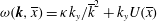
 $$\begin{eqnarray}\unicode[STIX]{x1D714}(\boldsymbol{k},x)=\frac{k_{y}[\unicode[STIX]{x1D705}+U^{\prime \prime }(x)]}{\overline{k}^{2}}+k_{y}U(x),\end{eqnarray}$$
where
 $\overline{k}^{2}=k^{2}+\unicode[STIX]{x1D70C}_{s}^{-2}$
and
$\overline{k}^{2}=k^{2}+\unicode[STIX]{x1D70C}_{s}^{-2}$
and
 $k^{2}=k_{x}^{2}+k_{y}^{2}$
. Many studies have ignored the
$k^{2}=k_{x}^{2}+k_{y}^{2}$
. Many studies have ignored the
 $U^{\prime \prime }$
term. We show the results so obtained have extremely limited applicability and demonstrate the importance of retaining
$U^{\prime \prime }$
term. We show the results so obtained have extremely limited applicability and demonstrate the importance of retaining
 $U^{\prime \prime }$
.
$U^{\prime \prime }$
.
We take the forcing to consist of statistically homogeneous white noise with covariance
 $F$
and dissipation to consist of a constant friction
$F$
and dissipation to consist of a constant friction
 $\unicode[STIX]{x1D707}$
. Viscosity is not necessary to regularize the dynamics in the quasi-linear system because there is no turbulent cascade. Direct numerical simulations of both the original system and the quasi-linear approximation exhibit steady zonal flows (Srinivasan & Young Reference Srinivasan and Young2012; Parker & Krommes Reference Parker and Krommes2013).
$\unicode[STIX]{x1D707}$
. Viscosity is not necessary to regularize the dynamics in the quasi-linear system because there is no turbulent cascade. Direct numerical simulations of both the original system and the quasi-linear approximation exhibit steady zonal flows (Srinivasan & Young Reference Srinivasan and Young2012; Parker & Krommes Reference Parker and Krommes2013).
The CE2 equations can be derived directly from the quasi-linear equations of motion. We quote the results (Srinivasan & Young Reference Srinivasan and Young2012; Parker & Krommes Reference Parker and Krommes2013):
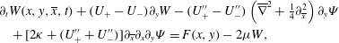 $$\begin{eqnarray}\displaystyle & & \displaystyle \unicode[STIX]{x2202}_{t}W(x,y,\overline{x},t)+(U_{+}-U_{-})\unicode[STIX]{x2202}_{y}W-(U_{+}^{\prime \prime }-U_{-}^{\prime \prime })\left(\overline{\unicode[STIX]{x1D6FB}}^{2}+{\textstyle \frac{1}{4}}\unicode[STIX]{x2202}_{\overline{x}}^{2}\right)\unicode[STIX]{x2202}_{y}\unicode[STIX]{x1D6F9}\nonumber\\ \displaystyle & & \displaystyle \quad +\,[2\unicode[STIX]{x1D705}+(U_{+}^{\prime \prime }+U_{-}^{\prime \prime })]\unicode[STIX]{x2202}_{\overline{x}}\unicode[STIX]{x2202}_{x}\unicode[STIX]{x2202}_{y}\unicode[STIX]{x1D6F9}=F(x,y)-2\unicode[STIX]{x1D707}W,\end{eqnarray}$$
 $$\begin{eqnarray}\displaystyle \unicode[STIX]{x2202}_{t}U(\overline{x},t)+\unicode[STIX]{x1D707}U=-\unicode[STIX]{x2202}_{\overline{x}}\unicode[STIX]{x2202}_{x}\unicode[STIX]{x2202}_{y}\unicode[STIX]{x1D6F9}(x,y,\overline{x},t)|_{(x,y)=(0,0)}, & & \displaystyle\end{eqnarray}$$
where
 $U$
is the zonal flow velocity,
$U$
is the zonal flow velocity,
 $U_{\pm }=U(\overline{x}\pm x/2,t)$
, and
$U_{\pm }=U(\overline{x}\pm x/2,t)$
, and
 $U^{\prime \prime }=\unicode[STIX]{x2202}_{\overline{x}}^{2}U$
. Here,
$U^{\prime \prime }=\unicode[STIX]{x2202}_{\overline{x}}^{2}U$
. Here,
 $\overline{x}$
is the inhomogeneity coordinate – if quantities are statistically homogeneous, there is no dependence on
$\overline{x}$
is the inhomogeneity coordinate – if quantities are statistically homogeneous, there is no dependence on
 $\overline{x}$
.
$\overline{x}$
.
 $W$
and
$W$
and
 $\unicode[STIX]{x1D6F9}$
are the two-point, one-time covariance of vorticity and streamfunction, respectively, and are related by
$\unicode[STIX]{x1D6F9}$
are the two-point, one-time covariance of vorticity and streamfunction, respectively, and are related by
 $W(x,y,\overline{x},t)=L_{+}L_{-}\unicode[STIX]{x1D6F9}(x,y,\overline{x},t)$
, where
$W(x,y,\overline{x},t)=L_{+}L_{-}\unicode[STIX]{x1D6F9}(x,y,\overline{x},t)$
, where
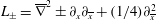 $L_{\pm }=\overline{\unicode[STIX]{x1D6FB}}^{2}\pm \unicode[STIX]{x2202}_{x}\unicode[STIX]{x2202}_{\overline{x}}+(1/4)\unicode[STIX]{x2202}_{\overline{x}}^{2}$
. Equivalently,
$L_{\pm }=\overline{\unicode[STIX]{x1D6FB}}^{2}\pm \unicode[STIX]{x2202}_{x}\unicode[STIX]{x2202}_{\overline{x}}+(1/4)\unicode[STIX]{x2202}_{\overline{x}}^{2}$
. Equivalently,
 $W$
is the physical-space Wigner function for
$W$
is the physical-space Wigner function for
 $\unicode[STIX]{x1D701}$
and (2.3a
) is the Wigner transport equation that can be alternatively described in terms of formal Weyl symbols (Krommes & Parker Reference Krommes, Parker, Galperin and Read2016). The right-hand side of (2.3b
) is the mean force due to the divergence of the Reynolds stress. Periodicity is assumed in
$\unicode[STIX]{x1D701}$
and (2.3a
) is the Wigner transport equation that can be alternatively described in terms of formal Weyl symbols (Krommes & Parker Reference Krommes, Parker, Galperin and Read2016). The right-hand side of (2.3b
) is the mean force due to the divergence of the Reynolds stress. Periodicity is assumed in
 $\overline{x}$
.
$\overline{x}$
.
3 Asymptotic wave-kinetic equation
A wave-kinetic equation (WKE) takes the form
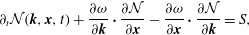 $$\begin{eqnarray}\unicode[STIX]{x2202}_{t}{\mathcal{N}}(\boldsymbol{k},\boldsymbol{x},t)+\frac{\unicode[STIX]{x2202}\unicode[STIX]{x1D714}}{\unicode[STIX]{x2202}\boldsymbol{k}}\boldsymbol{\cdot }\frac{\unicode[STIX]{x2202}{\mathcal{N}}}{\unicode[STIX]{x2202}\boldsymbol{x}}-\frac{\unicode[STIX]{x2202}\unicode[STIX]{x1D714}}{\unicode[STIX]{x2202}\boldsymbol{x}}\boldsymbol{\cdot }\frac{\unicode[STIX]{x2202}{\mathcal{N}}}{\unicode[STIX]{x2202}\boldsymbol{k}}=S,\end{eqnarray}$$
where
 ${\mathcal{N}}$
is the wave action density and
${\mathcal{N}}$
is the wave action density and
 $S$
represents sources and sinks (Connaughton, Nazarenko & Quinn Reference Connaughton, Nazarenko and Quinn2015; Krommes & Parker Reference Krommes, Parker, Galperin and Read2016). With
$S$
represents sources and sinks (Connaughton, Nazarenko & Quinn Reference Connaughton, Nazarenko and Quinn2015; Krommes & Parker Reference Krommes, Parker, Galperin and Read2016). With
 $S=0$
, it is Hamiltonian with
$S=0$
, it is Hamiltonian with
 $\unicode[STIX]{x1D714}$
generating the equations for wavepacket trajectories through phase space,
$\unicode[STIX]{x1D714}$
generating the equations for wavepacket trajectories through phase space,
 $\text{d}\boldsymbol{x}/\text{d}t=\unicode[STIX]{x1D735}_{\boldsymbol{k}}\unicode[STIX]{x1D714}$
and
$\text{d}\boldsymbol{x}/\text{d}t=\unicode[STIX]{x1D735}_{\boldsymbol{k}}\unicode[STIX]{x1D714}$
and
 $\text{d}\boldsymbol{k}/\text{d}t=-\unicode[STIX]{x1D735}_{\boldsymbol{x}}\unicode[STIX]{x1D714}$
. For the physical-space coordinates, we write
$\text{d}\boldsymbol{k}/\text{d}t=-\unicode[STIX]{x1D735}_{\boldsymbol{x}}\unicode[STIX]{x1D714}$
. For the physical-space coordinates, we write
 $\boldsymbol{x}=(\overline{x},\overline{y})\rightarrow \overline{x}$
because we only allow inhomogeneity in one direction.
$\boldsymbol{x}=(\overline{x},\overline{y})\rightarrow \overline{x}$
because we only allow inhomogeneity in one direction.
A form which has been used as the starting point in many geophysical and plasma physics studies assumes the zonal flows are asymptotically large scale relative to the fluctuations, in which case one neglects
 $U^{\prime \prime }$
in (2.2) and has
$U^{\prime \prime }$
in (2.2) and has
 $\unicode[STIX]{x1D714}(\boldsymbol{k},\overline{x})=\unicode[STIX]{x1D705}k_{y}/\overline{k}^{2}+k_{y}U(\overline{x})$
. Equation (3.1) becomes
$\unicode[STIX]{x1D714}(\boldsymbol{k},\overline{x})=\unicode[STIX]{x1D705}k_{y}/\overline{k}^{2}+k_{y}U(\overline{x})$
. Equation (3.1) becomes
 $$\begin{eqnarray}\unicode[STIX]{x2202}_{t}{\mathcal{N}}(\boldsymbol{k},\overline{x},t)-k_{x}U^{\prime }\frac{\unicode[STIX]{x2202}{\mathcal{N}}}{\unicode[STIX]{x2202}k_{x}}-\frac{2\unicode[STIX]{x1D705}k_{x}k_{y}}{\overline{k}^{4}}\frac{\unicode[STIX]{x2202}{\mathcal{N}}}{\unicode[STIX]{x2202}\overline{x}}=\frac{F(\boldsymbol{k})}{\unicode[STIX]{x1D705}}-2\unicode[STIX]{x1D707}{\mathcal{N}},\end{eqnarray}$$
where forcing and dissipation have been inserted and the wave action density is
 ${\mathcal{N}}=W/\unicode[STIX]{x1D705}$
.
${\mathcal{N}}=W/\unicode[STIX]{x1D705}$
.
We denote this system as the asymptotic WKE (Manin & Nazarenko Reference Manin and Nazarenko1994; Smolyakov, Diamond & Shevchenko Reference Smolyakov, Diamond and Shevchenko2000b ), which we shall see shortly is the limit of the CE2 equations in which the wavelength of zonal flow is taken to be asymptotically large. Justifications for the long-wavelength assumption are tenuous in magnetically confined plasmas, in which the characteristic size of zonal flows is often measured to be comparable to that of the turbulence (Fujisawa et al. Reference Fujisawa, Itoh, Iguchi, Matsuoka, Okamura, Shimizu, Minami, Yoshimura, Nagaoka and Takahashi2004; Gupta et al. Reference Gupta, Fonck, McKee, Schlossberg and Shafer2006; Hillesheim et al. Reference Hillesheim, Delabie, Meyer, Maggi, Meneses, Poli and Contributors2016). Furthermore, despite the use of the asymptotic WKE in the plasma literature over many years, to our knowledge it has never before been validated by comparing nonlinear numerical solutions to a parent model.
Various studies have inserted into the basic wave-kinetic equation a term that represents the effects of eddy–eddy nonlinear interactions. These interactions conserve energy and enstrophy. In a weak turbulence assumption, these effects can be derived in an asymptotic expansion (Nazarenko Reference Nazarenko2011). Simple analytic studies sometimes use an ad hoc nonlinear damping term such as
 $-{\mathcal{N}}^{2}$
, which balances linear instabilities that arise in various plasma models (Diamond et al.
Reference Diamond, Itoh, Itoh and Hahm2005). While retaining the effect of eddy–eddy nonlinear interactions in some form is important for many situations, it is unnecessary here. In the quasi-linear approximation, the eddy–eddy nonlinear interactions are absent, which is why an exact statistical theory could be formulated without a closure problem. The lack of eddy–eddy nonlinear interactions makes the quasi-linear system a useful testbed for various statistical theories and approximations of the drift wave–zonal flow problem. If a model is unable to faithfully reproduce the quasi-linear dynamics where these effects are absent, then one has no confidence in that model in the more realistic situation when these effects are included.
$-{\mathcal{N}}^{2}$
, which balances linear instabilities that arise in various plasma models (Diamond et al.
Reference Diamond, Itoh, Itoh and Hahm2005). While retaining the effect of eddy–eddy nonlinear interactions in some form is important for many situations, it is unnecessary here. In the quasi-linear approximation, the eddy–eddy nonlinear interactions are absent, which is why an exact statistical theory could be formulated without a closure problem. The lack of eddy–eddy nonlinear interactions makes the quasi-linear system a useful testbed for various statistical theories and approximations of the drift wave–zonal flow problem. If a model is unable to faithfully reproduce the quasi-linear dynamics where these effects are absent, then one has no confidence in that model in the more realistic situation when these effects are included.
Dynamics in the asymptotic WKE is closed by adding the equation for the zonal flow,
 $$\begin{eqnarray}\unicode[STIX]{x2202}_{t}U(\overline{x},t)+\unicode[STIX]{x1D707}U=\unicode[STIX]{x2202}_{\overline{x}}\int \frac{\text{d}\boldsymbol{k}}{(2\unicode[STIX]{x03C0})^{2}}\frac{\unicode[STIX]{x1D705}k_{x}k_{y}}{\overline{k}^{4}}{\mathcal{N}}(\boldsymbol{k},\overline{x},t),\end{eqnarray}$$
where we have used the Fourier transform convention
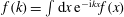 $f(k)=\int \text{d}x\,\text{e}^{-\text{i}kx}f(x)$
. With no forcing or dissipation, it conserves enstrophy within the fluctuations only and conserves total energy of the fluctuations and zonal flow.
$f(k)=\int \text{d}x\,\text{e}^{-\text{i}kx}f(x)$
. With no forcing or dissipation, it conserves enstrophy within the fluctuations only and conserves total energy of the fluctuations and zonal flow.
The asymptotic WKE is also poorly behaved at small scales. It drives growth of arbitrarily small-scale zonal flow in finite time, violating its fundamental assumption of scale separation as well as precluding any kind of well-behaved solution. The dispersion relation of zonostrophic instability for perturbations
 ${\sim}\text{e}^{\unicode[STIX]{x1D706}t}\text{e}^{\text{i}q\overline{x}}$
is shown in figure 2.
${\sim}\text{e}^{\unicode[STIX]{x1D706}t}\text{e}^{\text{i}q\overline{x}}$
is shown in figure 2.

Figure 2. Dispersion relation of zonostrophic instability describing linear stage of growth of zonal flows about a homogeneous equilibrium. Inset: zoomed in at small
 $q$
, where all the curves overlap. Parameters:
$q$
, where all the curves overlap. Parameters:
 $\unicode[STIX]{x1D707}=0.02$
,
$\unicode[STIX]{x1D707}=0.02$
,
 $\unicode[STIX]{x1D6FD}=1$
,
$\unicode[STIX]{x1D6FD}=1$
,
 $\unicode[STIX]{x1D70C}_{s}^{-2}=1$
,
$\unicode[STIX]{x1D70C}_{s}^{-2}=1$
,
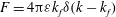 $F=4\unicode[STIX]{x03C0}\unicode[STIX]{x1D700}k_{f}\unicode[STIX]{x1D6FF}(k-k_{f})$
,
$F=4\unicode[STIX]{x03C0}\unicode[STIX]{x1D700}k_{f}\unicode[STIX]{x1D6FF}(k-k_{f})$
,
 $\unicode[STIX]{x1D700}=1$
,
$\unicode[STIX]{x1D700}=1$
,
 $k_{f}=1$
.
$k_{f}=1$
.
The dispersion relation plotted in figure 2 is calculated as follows. Equation (3.2) contains a homogeneous equilibrium, independent of
 $\overline{x}$
, at
$\overline{x}$
, at
 ${\mathcal{N}}_{H}=F/2\unicode[STIX]{x1D705}\unicode[STIX]{x1D707}$
,
${\mathcal{N}}_{H}=F/2\unicode[STIX]{x1D705}\unicode[STIX]{x1D707}$
,
 $U=0$
. One writes
$U=0$
. One writes
 ${\mathcal{N}}={\mathcal{N}}_{H}+\text{e}^{\text{i}q\overline{x}}\text{e}^{\unicode[STIX]{x1D706}t}{\mathcal{N}}_{1}(k_{x},k_{y})$
,
${\mathcal{N}}={\mathcal{N}}_{H}+\text{e}^{\text{i}q\overline{x}}\text{e}^{\unicode[STIX]{x1D706}t}{\mathcal{N}}_{1}(k_{x},k_{y})$
,
 $U=\text{e}^{\text{i}q\overline{x}}\text{e}^{\unicode[STIX]{x1D706}t}U_{1}$
and linearises. The linearised form of (3.2a
) can be solved for
$U=\text{e}^{\text{i}q\overline{x}}\text{e}^{\unicode[STIX]{x1D706}t}U_{1}$
and linearises. The linearised form of (3.2a
) can be solved for
 ${\mathcal{N}}_{1}$
in terms of
${\mathcal{N}}_{1}$
in terms of
 $U_{1}$
, and then substituted into (3.2b
), yielding a single nonlinear equation for the eigenvalue
$U_{1}$
, and then substituted into (3.2b
), yielding a single nonlinear equation for the eigenvalue
 $\unicode[STIX]{x1D706}$
:
$\unicode[STIX]{x1D706}$
:
 $$\begin{eqnarray}\unicode[STIX]{x1D706}+\unicode[STIX]{x1D707}=-q^{2}\int \frac{\text{d}\boldsymbol{k}}{(2\unicode[STIX]{x03C0})^{2}}\frac{k_{x}k_{y}^{2}}{(\unicode[STIX]{x1D706}+2\unicode[STIX]{x1D707})\overline{k}^{4}-2\text{i}\unicode[STIX]{x1D705}qk_{x}k_{y}}\unicode[STIX]{x1D705}\frac{\unicode[STIX]{x2202}{\mathcal{N}}_{H}}{\unicode[STIX]{x2202}k_{x}}.\end{eqnarray}$$
When
 $q$
is large, the unstable mode has
$q$
is large, the unstable mode has
 $\unicode[STIX]{x1D706}\sim q$
. Another solution exists where
$\unicode[STIX]{x1D706}\sim q$
. Another solution exists where
 $\unicode[STIX]{x1D706}$
is independent of
$\unicode[STIX]{x1D706}$
is independent of
 $q$
at large
$q$
at large
 $q$
, but this mode is typically damped and is of lesser physical interest. For more details, see appendix A and the supplementary material available at https://doi.org/10.1017/S0022377816001021.
$q$
, but this mode is typically damped and is of lesser physical interest. For more details, see appendix A and the supplementary material available at https://doi.org/10.1017/S0022377816001021.
Nonlinear simulations of the asymptotic WKE confirm the ultraviolet divergence. Figure 3 shows the spectrum of the zonal flow in the saturated, steady state for different values of the highest resolved wavenumber
 $q$
. No matter the resolution, the highest modes grow fastest and zonal flow energy concentrates in the highest resolved wavenumbers. For comparison, the figure also shows the same plot for a direct numerical simulation of the quasi-linear system, in which the scale of the zonal flow is not dependent on the numerical resolution. These simulations are pseudospectral, dealiased and nonlinearly conserve energy and enstrophy to machine precision.
$q$
. No matter the resolution, the highest modes grow fastest and zonal flow energy concentrates in the highest resolved wavenumbers. For comparison, the figure also shows the same plot for a direct numerical simulation of the quasi-linear system, in which the scale of the zonal flow is not dependent on the numerical resolution. These simulations are pseudospectral, dealiased and nonlinearly conserve energy and enstrophy to machine precision.

Figure 3. Spectrum of the zonal flow
 $U(q)$
(the Fourier transform of
$U(q)$
(the Fourier transform of
 $U(\overline{x})$
) in the nonlinear saturated state at
$U(\overline{x})$
) in the nonlinear saturated state at
 $t_{f}=6/\unicode[STIX]{x1D707}$
in simulations of the quasi-linear system and the asymptotic WKE. In each simulation, the zonal flows reach a steady state. For the asymptotic WKE, the results from three simulations are shown, with three different values for the maximum resolved wavenumber of the zonal flow. In each case, the zonal flow energy concentrates at the highest resolved wavenumbers. Same parameters as in figure 2.
$t_{f}=6/\unicode[STIX]{x1D707}$
in simulations of the quasi-linear system and the asymptotic WKE. In each simulation, the zonal flows reach a steady state. For the asymptotic WKE, the results from three simulations are shown, with three different values for the maximum resolved wavenumber of the zonal flow. In each case, the zonal flow energy concentrates at the highest resolved wavenumbers. Same parameters as in figure 2.
For very small
 $q$
, this model correctly predicts for zonostrophic instability that fluctuations provide an effective forcing proportional to
$q$
, this model correctly predicts for zonostrophic instability that fluctuations provide an effective forcing proportional to
 $q^{2}$
, a regime sometimes described in the literature. Figure 2 shows that at least for some parameters, the
$q^{2}$
, a regime sometimes described in the literature. Figure 2 shows that at least for some parameters, the
 $q^{2}$
regime only exists for extremely small
$q^{2}$
regime only exists for extremely small
 $q$
.
$q$
.
Early studies with the asymptotic WKE correctly deduced that the symmetry-breaking instability is likely a generic phenomenon, which was a key insight (Manin & Nazarenko Reference Manin and Nazarenko1994; Lebedev et al.
Reference Lebedev, Diamond, Shapiro and Soloviev1995; Krommes & Kim Reference Krommes and Kim2000; Smolyakov et al.
Reference Smolyakov, Diamond and Shevchenko2000b
). The asymptotic WKE has been used to predict growth rates of zonal flow in various systems (Diamond et al.
Reference Diamond, Rosenbluth, Hinton, Malkov, Fleischer and Smolyakov1998; Malkov, Diamond & Smolyakov Reference Malkov, Diamond and Smolyakov2001b
; Anderson et al.
Reference Anderson, Nordman, Singh and Weiland2002, Reference Anderson, Nordman, Singh and Weiland2006; Wang & Hahm Reference Wang and Hahm2009). As the above results indicate, predicted growth rates will be accurate only at small
 $q$
. Significant error occurs at moderate
$q$
. Significant error occurs at moderate
 $q$
, and crucially, the asymptotic WKE is completely unable to predict the wavenumber
$q$
, and crucially, the asymptotic WKE is completely unable to predict the wavenumber
 $q$
with maximum growth rate. Aside from growth rates, others have attempted to use the asymptotic WKE to seek nonlinear solutions of zonal flow–turbulence interaction, but due to the system’s tendency to dynamically generate small-scale flows, that is invalid from the start (Smolyakov et al.
Reference Smolyakov, Diamond and Malkov2000a
; Malkov & Diamond Reference Malkov and Diamond2001; Malkov, Diamond & Rosenbluth Reference Malkov, Diamond and Rosenbluth2001a
; Kaw, Singh & Diamond Reference Kaw, Singh and Diamond2002; Balescu Reference Balescu2003; Itoh et al.
Reference Itoh, Hallatschek, Toda, Itoh, Diamond, Yagi and Sanuki2004, Reference Itoh, Hallatschek, Itoh, Diamond and Toda2005; Trines et al.
Reference Trines, Bingham, Silva, Mendonça, Shukla and Mori2005; Singh et al.
Reference Singh, Singh, Kaw, Gürcan and Diamond2014). It appears only one of these studies (Trines et al.
Reference Trines, Bingham, Silva, Mendonça, Shukla and Mori2005) performs numerical simulations of the asymptotic WKE.
$q$
with maximum growth rate. Aside from growth rates, others have attempted to use the asymptotic WKE to seek nonlinear solutions of zonal flow–turbulence interaction, but due to the system’s tendency to dynamically generate small-scale flows, that is invalid from the start (Smolyakov et al.
Reference Smolyakov, Diamond and Malkov2000a
; Malkov & Diamond Reference Malkov and Diamond2001; Malkov, Diamond & Rosenbluth Reference Malkov, Diamond and Rosenbluth2001a
; Kaw, Singh & Diamond Reference Kaw, Singh and Diamond2002; Balescu Reference Balescu2003; Itoh et al.
Reference Itoh, Hallatschek, Toda, Itoh, Diamond, Yagi and Sanuki2004, Reference Itoh, Hallatschek, Itoh, Diamond and Toda2005; Trines et al.
Reference Trines, Bingham, Silva, Mendonça, Shukla and Mori2005; Singh et al.
Reference Singh, Singh, Kaw, Gürcan and Diamond2014). It appears only one of these studies (Trines et al.
Reference Trines, Bingham, Silva, Mendonça, Shukla and Mori2005) performs numerical simulations of the asymptotic WKE.
Approximations of the asymptotic WKE are perilous because they can elide the growth of small scales present in the model. Sometimes, a random-walk argument based on random zonal flows has been invoked to transform (3.2a ) into a diffusion equation (Diamond et al. Reference Diamond, Rosenbluth, Hinton, Malkov, Fleischer and Smolyakov1998; Malkov & Diamond Reference Malkov and Diamond2001). However, such an assumption stands in contrast with the typically real growth rate of zonal flows and the observations from numerical simulations of Hasegawa–Mima or Hasegawa–Wakatani models that exhibit steady, not random, zonal flows (Numata, Ball & Dewar Reference Numata, Ball and Dewar2007; Parker & Krommes Reference Parker and Krommes2013).
4 Geometrical optics approximations
We report two reductions of CE2 involving a geometrical optics approximation.
The first approximation, which we call CE2-GO, involves an expansion in space that is justified when inhomogeneities are weak. The
 $U_{\pm }$
terms in (2.3a
) are Taylor expanded for small
$U_{\pm }$
terms in (2.3a
) are Taylor expanded for small
 $x$
, assuming that the covariance
$x$
, assuming that the covariance
 $W$
is small when
$W$
is small when
 $x$
is not small. Additionally, only lowest order in
$x$
is not small. Additionally, only lowest order in
 $\unicode[STIX]{x2202}_{\overline{x}}$
is kept, e.g. the lowest-order relation
$\unicode[STIX]{x2202}_{\overline{x}}$
is kept, e.g. the lowest-order relation
 $W(x,y,\overline{x})=\overline{\unicode[STIX]{x1D6FB}}^{4}\unicode[STIX]{x1D6F9}(x,y,\overline{x})$
is used. After Fourier transforming
$W(x,y,\overline{x})=\overline{\unicode[STIX]{x1D6FB}}^{4}\unicode[STIX]{x1D6F9}(x,y,\overline{x})$
is used. After Fourier transforming
 $(x,y)\rightarrow \boldsymbol{k}$
, we obtain
$(x,y)\rightarrow \boldsymbol{k}$
, we obtain
 $$\begin{eqnarray}\displaystyle & \displaystyle \unicode[STIX]{x2202}_{t}W(\boldsymbol{k},\overline{x},t)-k_{y}U^{\prime }\frac{\unicode[STIX]{x2202}W}{\unicode[STIX]{x2202}k_{x}}-k_{y}U^{\prime \prime \prime }\frac{\unicode[STIX]{x2202}}{\unicode[STIX]{x2202}k_{x}}\left(\frac{W}{\overline{k}^{2}}\right)-2(\unicode[STIX]{x1D705}+U^{\prime \prime })\frac{k_{x}k_{y}}{\overline{k}^{4}}\frac{\unicode[STIX]{x2202}W}{\unicode[STIX]{x2202}\overline{x}}=F(\boldsymbol{k})-2\unicode[STIX]{x1D707}W,\qquad & \displaystyle\end{eqnarray}$$
 $$\begin{eqnarray}\displaystyle & \displaystyle \unicode[STIX]{x2202}_{t}U(\overline{x},t)+\unicode[STIX]{x1D707}U=\unicode[STIX]{x2202}_{\overline{x}}\int \frac{\text{d}\boldsymbol{k}}{(2\unicode[STIX]{x03C0})^{2}}\frac{k_{x}k_{y}}{\overline{k}^{4}}W. & \displaystyle\end{eqnarray}$$
The dispersion relation for zonally symmetric perturbations about a homogeneous equilibrium can be obtained in a similar manner as (3.3). The result is
 $$\begin{eqnarray}\unicode[STIX]{x1D706}+\unicode[STIX]{x1D707}=-q^{2}\int \frac{\text{d}\boldsymbol{k}}{(2\unicode[STIX]{x03C0})^{2}}\frac{k_{x}k_{y}^{2}}{(\unicode[STIX]{x1D706}+2\unicode[STIX]{x1D707})\overline{k}^{4}-2\text{i}\unicode[STIX]{x1D705}qk_{x}k_{y}}\frac{\unicode[STIX]{x2202}}{\unicode[STIX]{x2202}k_{x}}\left[\left(1-\frac{q^{2}}{\overline{k}^{2}}\right)W_{H}\right],\end{eqnarray}$$
where
 $W_{H}=F/2\unicode[STIX]{x1D707}$
. This dispersion relation is identical to (3.3) except for the factor of
$W_{H}=F/2\unicode[STIX]{x1D707}$
. This dispersion relation is identical to (3.3) except for the factor of
 $(1-q^{2}/\overline{k}^{2})$
. This factor, which arises from the
$(1-q^{2}/\overline{k}^{2})$
. This factor, which arises from the
 $U^{\prime \prime \prime }$
term in (4.1a
), provides the crucial cutoff at large
$U^{\prime \prime \prime }$
term in (4.1a
), provides the crucial cutoff at large
 $q$
.
$q$
.
In the second approximation, the zonal flow is assumed quasi-static, leading to conservation of wave action density
 ${\mathcal{N}}=W/(\unicode[STIX]{x1D705}+U^{\prime \prime })$
. A wave-kinetic equation in the form of (3.1) is derived from (4.1a
) by dividing by
${\mathcal{N}}=W/(\unicode[STIX]{x1D705}+U^{\prime \prime })$
. A wave-kinetic equation in the form of (3.1) is derived from (4.1a
) by dividing by
 $(\unicode[STIX]{x1D705}+U^{\prime \prime })$
. One obtains
$(\unicode[STIX]{x1D705}+U^{\prime \prime })$
. One obtains
 $$\begin{eqnarray}\displaystyle & \displaystyle \unicode[STIX]{x2202}_{t}{\mathcal{N}}(\boldsymbol{k},\overline{x},t)-k_{y}\left(U^{\prime }+\frac{U^{\prime \prime \prime }}{\overline{k}^{2}}\right)\frac{\unicode[STIX]{x2202}{\mathcal{N}}}{\unicode[STIX]{x2202}k_{x}}-2(\unicode[STIX]{x1D705}+U^{\prime \prime })\frac{k_{x}k_{y}}{\overline{k}^{4}}\frac{\unicode[STIX]{x2202}{\mathcal{N}}}{\unicode[STIX]{x2202}\overline{x}}=\frac{F(\boldsymbol{k})}{\unicode[STIX]{x1D705}+U^{\prime \prime }}-2\unicode[STIX]{x1D707}{\mathcal{N}},\qquad & \displaystyle\end{eqnarray}$$
 $$\begin{eqnarray}\displaystyle & \displaystyle \unicode[STIX]{x2202}_{t}U(\overline{x},t)+\unicode[STIX]{x1D707}U=\unicode[STIX]{x2202}_{\overline{x}}\int \frac{\text{d}\boldsymbol{k}}{(2\unicode[STIX]{x03C0})^{2}}\frac{k_{x}k_{y}}{\overline{k}^{4}}(\unicode[STIX]{x1D705}+U^{\prime \prime }){\mathcal{N}}. & \displaystyle\end{eqnarray}$$
 $U^{\prime \prime }$
is rapidly evolving such as during an instability because wave action is not conserved. This formulation therefore may not be used to study the dynamics in which a zonal flow evolves to a steady state. However, in the quasi-steady-state limit, the WKE is valid and equivalent to CE2-GO. The WKE exhibits a close connection to the Rayleigh–Kuo stability criterion, which states that a necessary condition for instability of fixed mean flow is that
$U^{\prime \prime }$
is rapidly evolving such as during an instability because wave action is not conserved. This formulation therefore may not be used to study the dynamics in which a zonal flow evolves to a steady state. However, in the quasi-steady-state limit, the WKE is valid and equivalent to CE2-GO. The WKE exhibits a close connection to the Rayleigh–Kuo stability criterion, which states that a necessary condition for instability of fixed mean flow is that
 $\unicode[STIX]{x1D705}+U^{\prime \prime }$
has a zero somewhere (Kuo Reference Kuo1949); such a condition would create singularities in
$\unicode[STIX]{x1D705}+U^{\prime \prime }$
has a zero somewhere (Kuo Reference Kuo1949); such a condition would create singularities in
 ${\mathcal{N}}=W/(\unicode[STIX]{x1D705}+U^{\prime \prime })$
.
${\mathcal{N}}=W/(\unicode[STIX]{x1D705}+U^{\prime \prime })$
.
Both CE2-GO and the WKE nonlinearly conserve enstrophy and energy between the fluctuations and zonal flow, although for the WKE one again must assume quasi-static zonal flow. Within the geometrical optics approximation, the energy density of the fluctuations is
 $(2L_{x})^{-1}\int _{0}^{L_{x}}\,\text{d}\overline{x}\int \,\text{d}\boldsymbol{k}(2\unicode[STIX]{x03C0})^{-2}W(\boldsymbol{k},\overline{x})/\overline{k}^{2}$
, and the enstrophy density is the same integral with
$(2L_{x})^{-1}\int _{0}^{L_{x}}\,\text{d}\overline{x}\int \,\text{d}\boldsymbol{k}(2\unicode[STIX]{x03C0})^{-2}W(\boldsymbol{k},\overline{x})/\overline{k}^{2}$
, and the enstrophy density is the same integral with
 $W$
instead of
$W$
instead of
 $W/\overline{k}^{2}$
, where
$W/\overline{k}^{2}$
, where
 $L_{x}$
is the periodicity length in the
$L_{x}$
is the periodicity length in the
 $x$
direction. The energy density of the zonal flow is
$x$
direction. The energy density of the zonal flow is
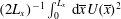 $(2L_{x})^{-1}\int _{0}^{L_{x}}\,\text{d}\overline{x}U(\overline{x})^{2}$
and the enstrophy density of the zonal flow is
$(2L_{x})^{-1}\int _{0}^{L_{x}}\,\text{d}\overline{x}U(\overline{x})^{2}$
and the enstrophy density of the zonal flow is
 $(2L_{x})^{-1}\int _{0}^{L_{x}}\,\text{d}\overline{x}U^{\prime }(\overline{x})^{2}$
. In the WKE, total wave action is conserved within the fluctuations under steady zonal flow and in the absence of forcing and dissipation.
$(2L_{x})^{-1}\int _{0}^{L_{x}}\,\text{d}\overline{x}U^{\prime }(\overline{x})^{2}$
. In the WKE, total wave action is conserved within the fluctuations under steady zonal flow and in the absence of forcing and dissipation.
In the limit of asymptotically large-scale zonal flows in which
 $U^{\prime \prime }$
and
$U^{\prime \prime }$
and
 $U^{\prime \prime \prime }$
are neglected, both CE2-GO and the WKE reduce to the asymptotic WKE.
$U^{\prime \prime \prime }$
are neglected, both CE2-GO and the WKE reduce to the asymptotic WKE.
The dispersion relations for zonostrophic instability in CE2-GO and the WKE are shown in figure 2. CE2-GO agrees remarkably well with the exact CE2, even at
 $q$
where a scale separation is not satisfied. The
$q$
where a scale separation is not satisfied. The
 $U^{\prime \prime \prime }$
term in (4.1a
) and (4.3a
) is essential; when only the flow shear
$U^{\prime \prime \prime }$
term in (4.1a
) and (4.3a
) is essential; when only the flow shear
 $U^{\prime }$
is retained, the dispersion relation grows linearly in
$U^{\prime }$
is retained, the dispersion relation grows linearly in
 $q$
. The WKE does not correctly predict the dispersion relation because its fundamental assumption of quasi-static zonal flow is violated.
$q$
. The WKE does not correctly predict the dispersion relation because its fundamental assumption of quasi-static zonal flow is violated.
We emphasize that CE2 is exact for quasi-linear dynamics while CE2-GO is approximate, so CE2-GO should not be preferred just because of its simpler and more intuitive form. Numerical solutions of CE2 are feasible and many studies have been carried out successfully (Farrell & Ioannou Reference Farrell and Ioannou2003, Reference Farrell and Ioannou2007; Marston et al. Reference Marston, Conover and Schneider2008; Tobias, Dagon & Marston Reference Tobias, Dagon and Marston2011; Parker & Krommes Reference Parker and Krommes2013; Constantinou et al. Reference Constantinou, Farrell and Ioannou2014; Parker & Krommes Reference Parker and Krommes2014; Squire & Bhattacharjee Reference Squire and Bhattacharjee2015). Moreover, numerically solving CE2 as compared to CE2-GO takes comparable effort as both are three dimensional, although the geometrical optics approximation may reduce the computational cost. Certain analytic calculations are also possible for CE2 (Srinivasan & Young Reference Srinivasan and Young2012; Bakas & Ioannou Reference Bakas and Ioannou2013; Parker & Krommes Reference Parker and Krommes2013, Reference Parker and Krommes2014; Bakas et al. Reference Bakas, Constantinou and Ioannou2015).
The utility of CE2-GO and the WKE, if they prove to be accurate, will come from their transparent phase-space formulation, more intuitive interpretation of wave dynamics, and greater possibility of analytic manipulation as compared to CE2. The WKE is valid for studying steady states, and we anticipate it will provide new insight into the behaviour of wavepackets in a steady mean flow.
5 Discussion
The asymptotic wave-kinetic equation, where zonal flows are assumed to be asymptotically large scale compared to the fluctuations, violates its own fundamental assumption in finite time. Within this model, the instability that drives zonal flows grows linearly in wavenumber without bound. Nonlinear numerical solutions confirm that zonal flow energy concentrates in the highest resolved wavenumbers. From one point of view, this ultraviolet divergence occurs because the asymptotic WKE attempts to describe the effect of mean flow on the fluctuations solely in terms of the local mean flow shear. Although the asymptotic WKE may remain useful as one of the simplest possible methods for investigating the linear stage of zonal flow growth, the CE2 and CE2-GO models offer more accurate yet still practicable methods that supersede it.
CE2 is an exact description of quasi-linear dynamics, and we have described two geometrical optics approximations that offer simpler and more intuitive phase-space equations. These formulations involve not only the local mean flow shear, but also the second and third derivative of the mean flow. The first formulation, CE2-GO, requires only a spatial scale expansion and agrees with the exact zonostrophic instability dispersion relation remarkably well. The second formulation, a wave-kinetic equation written in terms of conservation of wave action, is valid only when the zonal flow is slowly varying. This requirement precludes the use of the wave-kinetic equation for studying the important dynamics that determines how zonal flows grow and saturate, during which wave action is not conserved. Future work will continue to study the geometrical optics approximations and their validity.
While the quasi-linear approximation provides deep insight into the behaviour of zonal flows, it is important to understand when and why the approximation breaks down. For instance, Kelvin–Helmholtz-like instabilities of shear flow may limit their strength, and the quasi-linear approximation may not capture physics that depends on vortex roll up (Connaughton et al. Reference Connaughton, Nadiga, Nazarenko and Quinn2010). Comparisons of the quasi-linear system with higher fidelity models offers an approach of further developing our understanding of these kinds of effects. Initial efforts along these lines have been completed, but more remains to be understood (Tobias & Marston Reference Tobias and Marston2013; Constantinou et al. Reference Constantinou, Farrell and Ioannou2016; Marston, Chini & Tobias Reference Marston, Chini and Tobias2016)
Finally, although we have emphasized the quasi-linear approximation as a complete nonlinear system that can be analysed in detail, the geometrical optics approximation discussed here is useful more broadly. If one retained the effect of eddy–eddy nonlinearities, the geometrical optics approach may still be used to simplify the exact mean flow–fluctuation interactions.
Acknowledgements
Useful discussions with N. Constantinou, I. Dodin, J. Krommes, and D. Ruiz are acknowledged. The author is grateful for the helpful comments of an anonymous referee.
Supplementary material
Supplementary material is available at https://doi.org/10.1017/S0022377816001021.
Appendix A. Numerical calculation of dispersion relation
The dispersion relation for the zonostrophic instability in the asymptotic WKE, equation (3.3), and in CE2-GO, equation (4.2), can be solved numerically for the eigenvalue
 $\unicode[STIX]{x1D706}$
once the parameters
$\unicode[STIX]{x1D706}$
once the parameters
 $\unicode[STIX]{x1D6FD}$
,
$\unicode[STIX]{x1D6FD}$
,
 $\unicode[STIX]{x1D707}$
,
$\unicode[STIX]{x1D707}$
,
 $q$
and the forcing spectrum
$q$
and the forcing spectrum
 $F(\boldsymbol{k})$
are specified. In this appendix we explain the numerical calculation for
$F(\boldsymbol{k})$
are specified. In this appendix we explain the numerical calculation for
 $\unicode[STIX]{x1D706}$
shown in figure 2. We use the asymptotic WKE as an example; the calculation for the other models is analogous. Most choices of forcing
$\unicode[STIX]{x1D706}$
shown in figure 2. We use the asymptotic WKE as an example; the calculation for the other models is analogous. Most choices of forcing
 $F$
that result in an unstable perturbation
$F$
that result in an unstable perturbation
 $\text{Re}(\unicode[STIX]{x1D706})>0$
have a purely real
$\text{Re}(\unicode[STIX]{x1D706})>0$
have a purely real
 $\unicode[STIX]{x1D706}$
.
$\unicode[STIX]{x1D706}$
.
For the forcing
 $F$
, we take a thin-ring isotropic forcing
$F$
, we take a thin-ring isotropic forcing
 $F(k)=4\unicode[STIX]{x03C0}\unicode[STIX]{x1D700}k_{f}\unicode[STIX]{x1D6FF}(k-k_{f})$
, a convenient simplification. If
$F(k)=4\unicode[STIX]{x03C0}\unicode[STIX]{x1D700}k_{f}\unicode[STIX]{x1D6FF}(k-k_{f})$
, a convenient simplification. If
 $\unicode[STIX]{x1D70C}_{s}^{-2}=0$
, then
$\unicode[STIX]{x1D70C}_{s}^{-2}=0$
, then
 $\unicode[STIX]{x1D700}$
is equal to the energy input by the forcing. After integrating by parts in
$\unicode[STIX]{x1D700}$
is equal to the energy input by the forcing. After integrating by parts in
 $k_{x}$
, switching to polar coordinates
$k_{x}$
, switching to polar coordinates
 $k_{x}=k\cos \unicode[STIX]{x1D719}$
and
$k_{x}=k\cos \unicode[STIX]{x1D719}$
and
 $k_{y}=k\sin \unicode[STIX]{x1D719}$
, and integrating over the delta function, the dispersion relation becomes
$k_{y}=k\sin \unicode[STIX]{x1D719}$
, and integrating over the delta function, the dispersion relation becomes
 $$\begin{eqnarray}\unicode[STIX]{x1D706}+\unicode[STIX]{x1D707}=q^{2}\frac{\unicode[STIX]{x1D700}}{\unicode[STIX]{x1D707}}k_{f}^{4}(\unicode[STIX]{x1D706}+2\unicode[STIX]{x1D707})(1+m_{f})\int _{0}^{2\unicode[STIX]{x03C0}}\frac{\text{d}\unicode[STIX]{x1D719}}{2\unicode[STIX]{x03C0}}\frac{(1+m_{f}-4\cos ^{2}\unicode[STIX]{x1D719})\sin ^{2}\unicode[STIX]{x1D719}}{[(\unicode[STIX]{x1D706}+2\unicode[STIX]{x1D707})k_{f}^{2}(1+m_{f})^{2}-2\text{i}\unicode[STIX]{x1D705}q\cos \unicode[STIX]{x1D719}\sin \unicode[STIX]{x1D719}]^{2}},\end{eqnarray}$$
where
 $m_{f}=k_{f}^{-2}\unicode[STIX]{x1D70C}_{s}^{-2}$
. Assuming real
$m_{f}=k_{f}^{-2}\unicode[STIX]{x1D70C}_{s}^{-2}$
. Assuming real
 $\unicode[STIX]{x1D706}$
, one can rationalize the integrand and discard the imaginary part because it vanishes upon integration, and then proceed using robust one-dimensional numerical root finders.
$\unicode[STIX]{x1D706}$
, one can rationalize the integrand and discard the imaginary part because it vanishes upon integration, and then proceed using robust one-dimensional numerical root finders.
Python code to carry out the calculations and reproduce some of the curves in figure 2 is available in the supplementary material.


