


1. INTRODUCTION
Global Positioning System (GPS) -based attitude determination has been extensively investigated over the past twenty years and has proven to be an effective solution for attitude estimation (Cohen, Reference Cohen1992; Cannon et al., Reference Cannon, Sun, Owen and Meindl1994; Lu, Reference Lu1995; Wang, Reference Wang2003; Li et al., Reference Li, Liu, Lou and Zhou2007; Giorgi and Buist, Reference Giorgi and Buist2008; Giorgi et al., Reference Giorgi, Teunissen, Verhagen and Buist2010; Teunissen et. al., Reference Teunissen, Giorgi and Buist2011; Chen and Qin, Reference Chen and Qin2012). Because of its advantages of high precision, no error accumulation, low power consumption and low cost (Li and Yuan, Reference Li and Yuan2005; Wang et al., Reference Wang, Zhan and Zhang2007), GPS-based attitude determination has been widely used in a variety of applications on land, at sea, in air and space.
For a GPS-based attitude determination system, three or more GPS antennae are rigidly mounted to a platform and differential GPS measurements are collected simultaneously. This allows baseline vectors to be formed between antennae, and so the orientation of the platform can be calculated. Determination of baseline vectors with millimetre-level accuracy is usually achievable if the ambiguities can be resolved correctly. However, the measurements should be collected from two receivers at exactly the same time.
Typical GPS receivers collect measurements at regularly specified intervals and keep the individual internal clocks of oscillators synchronized with GPS time (Teunissen and Kleusberg, Reference Teunissen and Kleusberg1998). Simultaneous observations are performed by aligning the measurements of two receivers at the ‘same’ epoch. The receiver clock times (reading times), which are exactly known, are the same. If the two clocks involved are not synchronized, the true signal reception times of the two receivers at the same epoch are different due to the different receiver clock offsets. This results in a time misalignment, the magnitude of which is the difference of receiver clock offsets between the two receivers.
If there is a large time misalignment between two receivers, the calculated baseline vector actually refers to the vector between the antenna locations at different reception times. As a result it cannot be directly used to calculate the attitude parameters since this requires a “synchronized” baseline vector which can truly represent the platform orientation. Therefore, usually GPS receivers that share a common external oscillator are employed in dedicated GPS attitude determination systems (see e.g. Ashtech, 1991; Wilson and Tonnemacher, Reference Wilson and Tonnemacher1992; Hauschild and Montenbruck, Reference Hauschild and Montenbruck2007), so the observation times of the receivers are identical (i.e. the clocks of the two receivers are rigorously synchronized). In that case, the calculated baseline vector truly represents the baseline vector between antennae at the same time.
However, for many low-cost non-dedicated GPS attitude determination systems, each receiver utilises an independent oscillator and thus the two receivers are not synchronized and so the clock offsets of the two receivers are not identical. Consequently, the true signal reception times of the two receivers are not identical even though the measurements are performed at the same receiver clock time. For static cases, the locations of antennae remain unchanged between the true reception time and the receiver clock time, so there is no problem. But for kinematic cases, especially in high-kinematic applications, the locations of antennae can move significantly between the true reception time and the receiver clock time, which would lead to an offset in the baseline vector estimation. As a result of this, the calculated attitude parameters deviate from the true orientation of the platform. For precise airborne applications such as airborne photogrammetry, this can result in large errors in the exterior orientation parameters and thus lead to large imaging distortion. In order to eliminate the effects of time misalignment on attitude determination and to achieve accurate attitude parameters, the motion of the vehicles should be properly considered. Corrections should be made to the computed baseline vectors in order to compute the correct attitude of the platform from multiple GPS antenna arrays.
In this paper, we first investigate the generation of the problem. Then we investigate the influence of time misalignment on baseline vector estimation and attitude determination and propose two effective approaches to correct it, allowing accurate GPS-based attitude determination. The approaches are well suited for high-kinematic applications with low acceleration or low rate attitude changes. Finally real airborne GPS data processing is carried out to verify our approaches and results show that by using the proposed approaches the undesirable effects of the time misalignment between GPS receivers can be eliminated.
2. RECEIVER TIME MISALIGNMENT CORRECTION METHOD
We assume that the clock offsets for two receivers m, n are τ m and τ n at the same epoch T, which is the nominal signal reception time of the measurements for both receivers. Note that the time tags of the measurements for both receivers may be different due to the clock jumps, but this can be solved beforehand and for more details, the reader can refer to Kim and Lee (Reference Kim and Lee2012) and Guo and Zhang (Reference Guo and Zhang2014). For simplification, the time tags are assumed to be identical here. The receiver clock offset represents the difference between the receiver clock time (nominal time of signal reception, i.e. time tag T) and true time of signal reception (t m and t n). The receiver clock offset can be determined easily by Standard Point Positioning (SPP) with pseudo-range measurements. We denote the true signal reception times as t m and t n for two receivers m, n respectively, so we have the following equation:
 $$t_m = T - \tau _m, {\rm} t_n = T - \tau _n $$
 In practice, the clocks of the two receivers involved are not usually exactly synchronized, i.e. τ m is not equal to τ n, which means that t m is not equal to t n, i.e. the true signal reception times of the two receivers at the same epoch are different. In this case, the baseline vector which is calculated from the raw measurements is actually the vector  $\vec B(t_m, t_n )$ from the position of the receiver m at time t m to the position of the receiver n at time t n. It cannot be directly used to calculate the attitude parameters since this requires the “synchronized” baseline vector which can truly represent the platform orientation, which means that the true signal reception times of the two receivers must be exactly identical. In order to address this problem, two approaches are presented in this paper as follows.
2.1. Correcting raw measurements
The Zero-Differenced (ZD) carrier phase observation equation between receiver m and two satellites i, j at time t m is given as (Teunissen and Kleusberg, Reference Teunissen and Kleusberg1998):
 $$\eqalign{& \phi _m^i (t_m ) = \rho _m^i (t_m, t^i ) - c \cdot (\tau _m - \tau ^i ) - \lambda \cdot N_m^i - I_m^i - Z_m^i + \varepsilon _m^i \cr & \phi\kern2pt _m^j (t_m ) = \rho\kern1.3pt _m^j (t_m, t\kern1pt^j ) - c \cdot (\tau _m - \tau ^j ) - \lambda \cdot N_m^j - I_m^j - Z_m^j + \varepsilon \kern1.5pt_m^j} $$
where λ is the wavelength, c is the speed of light in vacuum, φ are the carrier phase measurements in metres, ρ is the geometric range from satellite to receiver, N is the ambiguity, t m is the true sampling time, τ m is the receiver clock offset, ti is the signal transmitting time, τi is the satellite clock bias, I, Z are ionospheric delay and tropospheric delay respectively. Errors such as antenna phase centre offset and phase centre variation, etc. can be corrected by models, so they are not presented in the equation. ε contains all remaining un-modelled effects and the observation noise.
Similarly, the ZD carrier phase observation equation between receiver n and two satellites i, j at time t n is given as:
 $$\eqalign{& \phi _n^i (t_n ) = \rho _n^i (t_n, t^i ) - c \cdot (\tau _n - \tau ^i ) - \lambda \cdot N_n^i - I_n^i - Z_n^i + \varepsilon _n^i \cr & \phi \kern2pt_n^j (t_n ) = \rho \kern1.3pt_n^j (t_n, t\kern2pt^j ) - c \cdot (\tau _n - \tau \kern1pt^j ) - \lambda \cdot N_n^j - I_n^j - Z_n^j + \varepsilon\kern1.3pt _n^j} $$
When the clocks of receiver m and receiver n are not synchronized, the true signal reception times of the two receivers are not identical (i.e. t m ≠ tn). However, we must use observations of both receivers at exactly the same signal reception time to compute the attitude of vehicles. In that case, taking into account the movement of the receivers, we first reduce the raw measurements from two receivers to the same signal reception time T. Then the corrected measurements can be used to compute the baseline vector between receivers.
As shown in Figure 1, accounting for the movement of receiver m during the time offset τ m and the fact that the movement is fairly short with respect to the geometric range from satellite to receiver, the reduced measurement from satellite i to receiver m at time T (true signal reception time) can be approximated as:
 $$\phi _m^i (T) \approx \phi _m^i (t_m ) + \vec v_m (t_m ) \cdot \vec e_m^i \cdot \tau _m $$
Figure 1. Correction of raw measurement considering the movement of the receiver.
where  $\vec v_m $ is the mean velocity of receiver m between time t m and t m + τ m, estimated from Doppler measurements at t m for approximation (Xu, Reference Xu2003), $\vec e_m^i $ is the unit vector from satellite i to receiver m at time t m.
From Equation (2) and Equation (4), the ZD carrier phase observation equation between receiver m and satellite i at time T (true signal reception time) is given as:
 $$\phi _m^i (T) \approx \phi _m^i (t_m )\;{\rm +}\; \vec v_m (t_m ) \cdot \vec e_m^i \cdot \tau _m = \rho _m^i (T,t^i ) - c \cdot (\tau _m - \tau ^i ) - \lambda \cdot N_m^i - I_m^i - Z_m^i + \varepsilon _m^i $$
Similarly, the ZD carrier phase observation equation between receiver n and satellite i at time T (true signal reception time) is given as:
 $$\phi _n^i (T) \approx \phi _n^i (t_n ) + \vec v_n (t_n ) \cdot \vec e_n^i \cdot \tau _n = \rho _n^i (T,t^i ) - c \cdot (\tau _n - \tau ^i ) - \lambda \cdot N_n^i - I_n^i - Z_n^i + \varepsilon _n^i $$
Double-Differenced (DD) measurements are generally formed to cancel out the satellite and receiver clock errors and mitigate the ionospheric and tropospheric delays. In attitude determination systems, due to the short separations between antennae, the residual ionospheric and tropospheric errors can be neglected. Thus DD carrier phase measurements between two satellites i, j and two receivers m, n at time T can be given as:
 $$\eqalign{&\nabla \Delta \phi _{mn}^{ij} (T) \approx \nabla \Delta \phi _{mn}^{ij} (t_m, t_n ) + [(\vec e_n\,\!\!^{j} \cdot \vec v_n (t_n ) \cdot \tau _n - \vec e_n^i \cdot \vec v_n (t_n ) \cdot \tau _n ) - (\vec e_m\,\!\!\!^{j} \cdot \vec v_m (t_m ) \cr &\quad\cdot \tau _m - \vec e_m^i \cdot \vec v_m (t_m ) \cdot \tau _m )] = \nabla \Delta \rho _{mn}^{ij} (T) - \lambda \cdot \nabla \Delta N_{mn}^{ij} + \nabla \Delta \varepsilon _{mn}^{ij}} $$
In Equation (7), the receiver clock error terms (the last term on the right of the first row of the equation) cannot be cancelled out by the double-difference technique. In static cases, the velocities of receivers are zero, thus the receiver clock terms are negligible. Without considering these receiver clock terms, the standard DD model can be given as:
 $$\nabla \Delta \phi _{mn}^{ij} (t_m, t_n ) = \nabla \Delta \rho _{mn}^{ij} (t_m, t_n ) - \lambda \cdot \nabla \Delta N_{mn}^{ij} + \nabla \Delta \varepsilon _{mn}^{ij} $$
 In kinematic cases, in order to make the following analysis simpler and clearer, two reasonable assumptions are made in this paper: 1) As the antenna array is mounted on a rigid platform such as an aircraft or ship in GPS attitude determination systems, the velocities of both receivers are identical at the same time (note that they will actually be unequal if there is a rotation of the platform. However, the difference between the two receivers' speed is generally very small); 2) The velocities of the antennae vary insignificantly during the fairly short time interval (between the true signal reception time and the receiver clock time, i.e. τ m and τ n). Under the above two assumptions, the velocities of antennae can be represented by the velocity of the vehicle and we can denote 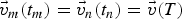 $\vec v_m (t_m ) = \vec v_n (t_n ) = \vec v(T)$. If the clock offsets of the two receivers are identical, i.e. τ m = τ n = τ, the receiver clock error terms can be approximated as:
 $$\eqalign{& (\vec e\kern2pt_n^j \cdot \vec v_n (t_n ) \cdot \tau _n - \vec e_n^i \cdot \vec v_n (t_n ) \cdot \tau _n ) - (\vec e\kern2pt_m^j \cdot \vec v_m (t_m ) \cdot \tau _m - \vec e\kern2pt_m^i \cdot \vec v_m (t_m ) \cdot \tau _m ) \cr & = {\rm [(}\vec e\kern2pt_n^j - \vec e\kern2pt_m^j ) - (\vec e\kern2pt_n^i - \vec e\kern2pt_m^i )] \cdot \vec v(T) \cdot \tau \cr & \approx 0} $$
It can be concluded from Equation (9) that the receiver clock error terms can also be neglected in case of identical clock offsets of receivers.
However, if the clock offsets of the two receivers are not identical, the receiver clock error terms can be given as:
 $$\eqalign{& (\vec e\kern1.5pt_n^j \cdot \vec v_n (t_n ) \cdot \tau _n - \vec e_n^i \cdot \vec v_n (t_n ) \cdot \tau _n ) - (\vec e\kern1.5pt_m^j \cdot \vec v_m (t_m ) \cdot \tau _m - \vec e\kern1.5pt_m^i \cdot \vec v_m (t_m ) \cdot \tau _m ) \cr & {\rm = (}\vec e\kern1.5pt_n^j - \vec e_n^i ) \cdot \vec v(T) \cdot \tau _n - (\vec e\kern1.5pt_m^j - \vec e\kern1.5pt_m^i ) \cdot \vec v(T) \cdot \tau _m} $$
The receiver clock error terms cannot be cancelled in Equation (10). For high-kinematic attitude determination cases, the receiver clock error terms can result in time-varying offsets in the baseline estimation (Buist et al., Reference Buist, Teunissen and Giorgi2010). In such cases, Equation (7) should be used to resolve the baseline parameters between antennae. However, from Equation (7), the definite impact of receiver clock terms on baseline estimation is implicit. In Section 2.2, we will discuss this problem from another point of view and the definite impact of receiver clock terms on baseline estimation will be presented.
2.2. Correcting the baseline vector
According to the relative positioning principle as shown in Figure 2, if the standard DD model is used, the baseline vector which is calculated from the raw measurements is actually the vector  $\vec B(t_m, t_n )$ between the position of receiver m at time t m and the position of receiver n at time t n:
 $$\vec B(t_m, t_n ) = \vec P_n (t_n ) - \vec P_m (t_m )$$
where  $\vec P_m (t_m )$ and $\vec P_n (t_n )$ denote the position of receiver m at time t m and position of receiver n at time t n respectively.

Figure 2. Baseline vector in relative positioning.
However, we use the baseline vector  $\vec B(T,T)$ between the two GPS antennae at the same nominal time tag to compute the attitude of vehicles. Therefore, corrections due to the time misalignment between the two receivers are made in order to obtain the baseline vector $\vec B(T,T)$. By taking the time misalignment into account, the position of two receivers m, n at time T can be given by:
 $$\vec P_m (T) = \vec P_m (t_m + \tau _m ) = \vec P_m (t_m ) + \vec v_m (t_m ) \cdot \tau _m $$
 $$\vec P_n (T) = \vec P_n (t_n + \tau _n ) = \vec P_n (t_n ) + \vec v_n (t_n ) \cdot \tau _n $$
where  $\vec v_m (t_m )$ represents the mean velocity of receiver m between time t m and t m + τ m, estimated from Doppler measurements at t m for approximation, and the same for $\vec v_n (t_n )$.
The baseline vector  $\vec B(T,T)$ at time T can be calculated with the following equation:
 $$\vec B(T,T) = \vec P_n (T) - \vec P_m (T)$$
Substituting Equations (12) and (13) into Equation (14), we have:
 $$\vec B(T,T) = \vec B(t_m, t_n ) + \Delta \vec B$$
where  $\Delta \vec B = \vec v(t_n ) \cdot \tau _n - \vec v(t_m ) \cdot \tau _m $.
In order to make the sequel analysis simpler and clearer, the same two assumptions regarding the velocities of the antennae are made here as in Section 2.1. In that case, we have:
 $$\vec v_n (t_n ) = \vec v_m (t_m ) = \vec v(T)$$
 Thus  $$\Delta \vec B$ can be simplified to
 $$\Delta \vec B = \vec v(T) \cdot (\tau _n - \tau _m )$$
It can be clearly seen from Equation (17) that the baseline estimation offset depends on the velocity of the vehicles and the time misalignment error between receivers. However, it is based on the assumption that the velocities of both receivers are identical at the same time and the velocities of the antennae vary insignificantly between the true signal reception time and the receiver clock time. Actually, as satellites are in motion around the Earth and the Global Navigation Satellite System (GNSS) antennae are also mounted on a moving platform, the sensed Doppler shift is a function of time, and its observed value will vary from one measurement instant to another (from one receiver to another). In the data processing procedure, the velocities of each receiver are calculated using Doppler measurements of the corresponding receiver epoch-wise. The velocity also varies from one measurement instant to another and from one receiver to another. For high kinematic vehicles with low velocity change (low acceleration) and low rate attitude changes, the approaches presented in this paper can effectively eliminate the time misalignment error without introducing large additional errors from neglecting the velocity differences. Thus our approaches can achieve remarkable results in such cases. However, if the vehicle is moving with high velocity changes (high acceleration) or high attitude changes, the assumptions may be invalid and the approaches may be restricted. Note also that the Least-Squares Ambiguity Decorrelation Adjustment (LAMBDA) method (Teunissen, Reference Teunissen1995) is used for integer ambiguity resolution and the baseline length constraint is used for ambiguity validation.
Experimental tests show that we can achieve similar results using either approach previously presented. Therefore, we do not make a distinction between the two approaches in Section 4.
3. INFLUENCE OF TIME MISALIGNMENT ON BASELINE VECTOR AND ATTITUDE DETERMINATION
Equation (17) shows that the correction term is proportional to the velocity of moving vehicles and the time misalignment between the receivers. Figure 3 shows the baseline offsets introduced by the time misalignments of different receivers with different velocities. For static cases,  $\Delta \vec B$ is equal to zero, which means that the time misalignment error can be ignored. For low-kinematic cases, the impact of the time misalignment is not significant if the time misalignment is smaller than 0·5 ms. For cases with high vehicle speeds, the baseline vector offset can be up to 5 cm, if the velocity is 50 m/s and time misalignment is 1 ms.

Figure 3. Baseline vector offsets introduced by different time misalignments with different velocities.
Receiver clock offsets are often less than a few milliseconds, which may result in a clock jump in many receivers. This depends on the clock steering mechanisms adopted by receivers. These can be divided into two categories. One is continuous steering, in which case the clock offset is generally kept within a few μs (e.g., NovAtel Smart 3100 IS and South NGS-9600 et al.). The other introduces discrete jumps into the receiver's estimate of time; e.g., Trimble 4700 and South Ashtech CH Z-XII3 et al., jumps typically occur when the clock offset exceeds 1 ms in magnitude (Kim and Langley, Reference Kim and Langley2001; Kim and Lee, Reference Kim and Lee2009, 2012; Guo and Zhang, Reference Guo and Zhang2014).
For a single baseline attitude determination system, once the baseline vector between the two antennae is determined, yaw and pitch can be calculated by a direct computation method as:
 $$y = \arctan (e/n)$$
 $$p = \arctan ({u / {\sqrt {(e^2 + n^2 )}}} )$$
where(e, n, u) denotes the baseline vector in the local horizontal coordinate frame with the origin at the master antenna.
The influence of baseline error on the computed yaw and pitch can be derived by differentiating Equations (18) and (19):
 $${\rm d}y = \displaystyle{{n\,{\rm d}e{\rm} - {\rm} e\,{\rm d}n} \over {n^2 + e^2}} = \displaystyle{{{\rm cos(}y{\rm ) d}e{\rm} - {\rm sin(}y{\rm ) d}n} \over {l\cos (\,p)}}$$
 $$\eqalign{{\rm d}p &= - \displaystyle{{ue} \over {(e^2 + n^2 + u^2 )\sqrt {e^2 + n^2}}} {\rm d}e - \displaystyle{{un} \over {(e^2 + n^2 + u^2 )\sqrt {e^2 + n^2}}} {\rm d}n + \displaystyle{{\sqrt {e^2 + n^2}} \over {e^2 + n^2 + u^2}} {\rm d}u \cr & = - \displaystyle{{\sin (\,p)\sin (y)} \over l}{\rm d}e - \displaystyle{{\sin (\,p)\cos (y)} \over l}{\rm d}n + \displaystyle{{\cos (\,p)} \over l}{\rm d}u}$$
where l is the length of the baseline, y is the yaw and p is the pitch.
According to Equations (20) and (21), the definite influence of baseline error on the computed yaw and pitch is inversely proportional to the baseline length; as well as depending on the baseline error and the attitude of the moving vehicle.
Moreover, considering Cauchy–Schwarz inequality, it can be deduced from Equations (20) and (21) that:
 $${\rm d}y \le \displaystyle{{{\rm d}l^{\prime}} \over {l\cos (\,p)}},{\rm d}p \le \displaystyle{{{\rm d}l} \over l}$$
Where  ${\rm d}l = \sqrt {({\rm d}e)^2 + ({\rm d}n)^2 + ({\rm d}u)^2} $ denotes the baseline error and ${\rm d}l' = \sqrt {({\rm d}e)^2 + ({\rm d}n)^2} $ denotes the horizontal baseline error.
From Equation (22), the maximum angular error is proportional to the baseline error and inversely proportional to the baseline separation. The maximum angular errors under different baseline separations with 1 ms time misalignment between receivers are calculated and shown in Figure 4. It can be seen that the angular error decreases dramatically as the baseline length increases. The angular error is extremely significant if the baseline length is shorter than 6 m (e.g., it can be as much as ~3·0o with a baseline separation of 1 m for a vehicle with 50 m/s velocity). Due to the limited installation space on vehicles, the baseline separation in most attitude determination systems is generally fairly short. Thus, receiver time misalignment compensation must be properly considered.

Figure 4. Maximum angular errors for 1 ms time misalignment at different velocities.
4. EXPERIMENTAL RESULTS AND ANALYSIS
In this section, two independent high-kinematic airborne experiments (with respect to vehicles on land or at sea) were carried out to verify the performance of our methods. First, we set up the experiments by using airborne zero baselines (one antenna shared by two independent receivers) to demonstrate the baseline vector offsets introduced by time misalignment. This allows the baseline vector correction to be quantified accurately because the true value of baseline vector is zero. In the second experiment we implemented a non-zero baseline case to demonstrate the influence of receiver time misalignment on attitude determination.
4.1. Airborne Experiment 1
The experiment was performed on 3 August 2005 to collect LIDAR measurements in Greenland, and the flight took off at 9:53 UTC and landed at 13:30 UTC. Two receivers (TPS LEGACY and TPS EGGDT) with different oscillators were used and shared a common GPS antenna on the aircraft. The aircraft made turns, climbs and descents several times during the flight and the flight trajectory is depicted in Figure 5.

Figure 5. Aircraft flight path (left) and altitude profile (right).
The number of satellites tracked and the HDOP/VDOP is shown in Figure 6 to illustrate the observation conditions and satellite geometry.

Figure 6. The number of satellites in view and HDOP/VDOP plot.
Figure 7 shows the clock offsets of the two receivers, calculated through SPP using pseudo-range measurements. In the figure it can be seen that the clock offsets of the two receivers were kept within 0·5 ms and the time misalignment between the two receivers varied smoothly during the experiment, except for the epoch near the beginning where a clock jump occurs on the TPS EGGDT receiver.
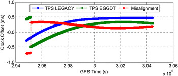
Figure 7. Clock offsets and the time misalignment of the receivers.
Figures 8 and 9 show the baseline errors in east and north directions without making receiver time misalignment correction. It can be seen that the variation of baseline error is correlated with the variation in the velocity of the vehicle; the higher the velocity, the larger the baseline error. Subsequently, no significant baseline vector errors occurred at the beginning, because the aircraft did not take off during this period. Figure 10 shows the vertical component in the baseline errors without correction for receiver time misalignment. There is no significant vertical error because the vertical flight velocity is very low.

Figure 8. The baseline errors with respect to flight velocities in the East without correcting for time misalignments.

Figure 9. The baseline errors with respect to flight velocities in the North without correcting for time misalignments.

Figure 10. The baseline errors with respect to vertical flight velocities without correcting for time misalignments.
Figure 11 shows the baseline errors after correcting receiver time misalignment. The magnitudes of each component are below 1 cm therefore the influence of time misalignment on baseline estimation is completely removed. By comparing Figures 8 and 9 and Figure 11, it can be concluded that the proposed approaches can effectively eliminate the undesirable effects from receiver time misalignment.
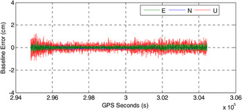
Figure 11. The baseline errors after correcting for time misalignments.
In the above airborne zero-baseline experiment, if the true signal reception times of two receivers are identical, the baseline vector we obtain should be close to zero. However, the true signal reception times of the two receivers are actually not identical. As the aircraft moves very fast, the antenna position changes quickly even over a very short time (e.g. 1 ms). The positions of the antenna are not the same at different reception times and so the computed baseline vector actually refers to a displacement vector between the positions of the same antenna at different reception times. Therefore, the computed baseline length is definitely not zero.
4.2. Airborne Experiment 2
The second experiment was conducted on 4 July 2003 while making an airborne LIDAR survey of the sea-ice freeboard in the North Atlantic. The flight took off at 13:07 UTC at Höfn, Iceland and landed at 18:09 UTC at Stornoway, Outer Hebrides, Scotland. Three receivers, TRIMBLE 4000SSI, ASHTECH UZ-12 and JPS LEGACY and two antennae were used on the aircraft. The TRIMBLE 4000SSI and ASHTECH UZ-12 had different oscillators but shared a common GPS antenna, while the JPS LEGACY was connected to another antenna. The baseline separation between the two antennae was 3·79 m.
The flight trajectory and flight profile in height is depicted in Figure 12. The number of satellites in view and the HDOP/VDOP during the flight are shown in Figure 13. The three-dimensional velocities of the aircraft, which were calculated from Doppler measurements, are shown in Figure 14.

Figure 12. Aircraft flight path (left) and altitude profile (right).

Figure 13. The number of satellites in view and the HDOP/VDOP during the flight.

Figure 14. Velocities of the aircraft.
4.2.1. Zero Baseline Results
Figure 15 shows the clock offsets of the two receivers and the time misalignment between them during the flight. The receiver clock offsets of ASHTECH UZ-12 are small while that of TRIMBLE 4000SSI experiences periodic saw-tooth shaped behaviour and can reach a maximum value of about 1 ms. There are significant time misalignments between the two receivers.

Figure 15. Clock offsets and time misalignments of receivers.
Figure 16 shows the time series of baseline vectors without correction of receiver time misalignment. The true baseline vector should be close to zero as the two receivers shared the same antenna. However, due to the time misalignment, the calculated baseline vector is not close to zero. From Figures 14, 15 and 16, we observe that the calculated baseline vector changes with the time misalignments as well as the velocities. The baseline errors are proportional to the magnitude of time misalignments and velocities. The baseline errors in the East and North vary periodically in saw-tooth-like shapes and are closely correlated with the variation of the time misalignment between the two receivers. This is reasonable, because the aircraft was moving steadily with a velocity of about 50 m/s in the North and East respectively for most of the flight period. At the beginning and end of the flight, the velocities of the aircraft are small, thus the baseline vector errors are close to zero. There are no significant errors in the vertical direction, since the vertical velocity is not significant.

Figure 16. Baseline errors without correction of receiver time misalignment errors.
Figure 17 shows the baseline vector errors after applying the receiver time misalignment compensation. It can be seen that the errors in each component are below 1 cm in most cases and the time-varying offsets for the baseline solution are almost completely removed. Comparing Figure 16 with Figure 17, it can be concluded that the proposed approaches can effectively eliminate the undesirable effects of receiver time misalignment. However, the vertical component is noisier than the horizontal components due to the larger uncertainties of the height components as determined by the GPS technique.

Figure 17. Baseline vector errors after receiver time misalignment error correction.
4.2.2. Non-zero Baseline Results
Two non-zero baseline vectors are calculated in this experiment. One is the displacement vector between receiver TRIMBLE 4000SSI and JPS LEGACY and the other is the vector between ASHTECH UZ-12 and JPS LEGACY. The results (i.e. baseline vector and yaw/pitch) presented here are related to the first displacement vector mentioned. In order to verify the performance of our method, we make a comparison of the results with and without time misalignment correction.
Figure 18 shows the clock offsets of the two receivers and their time misalignments during the flight. The variation trend of time misalignment between the two receivers is similar to that of the zero-baseline case.

Figure 18. Clock offsets and time misalignments of receivers.
Figure 19 shows the differences of the baseline vectors with and without receiver time misalignment compensation. The variation trend is similar to that of the zero-baseline case and so it will not be discussed further here. The maximum difference between the baseline vectors can reach about 10 cm, which is equivalent to an attitude error of about 1·5o with a baseline length of 3·79 m. This is the maximum bias that can occur. The actual biases in the yaw/pitch are related to the attitude of the baseline vector and the biased vector. Although they are usually smaller than the maximum biases, they can still be significant and thus cannot be neglected.

Figure 19. Differences of baseline vectors with and without time misalignment correction.
Figure 20 shows the differences of yaw/pitch with and without receiver time misalignment correction. It can be seen that the differences also show periodic behaviour. The maximum difference can reach about 0·5o in the yaw and 0·1o in the pitch respectively. These biases are unacceptable for precise attitude determination applications. These magnitudes correspond to our specific experiment with a baseline separation of 3·79 m. In many practical applications, however, the baseline separations are smaller due to the limited space of the platform. In such cases, the biases will be even more significant. Therefore, the receiver time misalignment should be properly compensated for high-kinematic attitude determination systems with short baseline separations.

Figure 20. Differences of yaw/pitch with and without correcting for time misalignment.
4.3. Discussion
In relative positioning, typical GPS receivers record measurements at regularly specified intervals and keep the individual internal clocks of oscillators synchronized with GPS time. We generally regard the same receiver clock time measurements of two involved receivers as simultaneous observations when calculating the baseline vectors. However, as the receivers often use different oscillators, the same receiver clock time of two measurements does not mean that they are simultaneous. For GPS receivers with continuous clock steering mechanisms, the time misalignment between receivers is not significant as the receiver clock is synchronized to GPS time at every epoch. Nevertheless, the clock offsets of GPS receivers with clock jumping can easily reach a few milliseconds, because the receiver's oscillator is not calibrated at every epoch; instead it is reset when the clock drift reaches a certain limit (Hoyle et al., Reference Hoyle, Lachapelle, Cannon and Wang2002).
In principle, it is not essential that exactly simultaneous measurements should be used as long as all errors can be reduced to a negligible level when the double differences are made. Whether the influence of time misalignment on baseline vector computation is taken into consideration depends on the application for which the baseline vector is being calculated. Currently, the time misalignment between receivers is ignored for most applications. For static or low-kinematic cases, the effect is insignificant, so it could be ignored. However, for applications involving vehicles moving with high speeds, the time misalignment cannot be ignored if accurate baseline vectors need to be achieved.
In GPS-based attitude determination systems, the exact baseline vector should be derived from two antenna positions at precisely the same time. Therefore, if the time misalignment between receivers is not properly compensated for, a baseline vector offset will be introduced and thus it will deteriorate the value of attitude parameters. Taking Airborne Experiment 2 as an example, the baseline vector offset often reaches about 5 cm, which is equivalent to an attitude bias of about 2·8o for a baseline length of 1 m (Note that the bias to which we refer here corresponds to the maximum bias that can occur). These biases are unacceptable for precise attitude determination applications.
Spacecraft formation flying is another set of applications for which the time misalignment between receivers should be properly considered. For spacecraft formation flying, the influence of the effect is normally kept small by keeping the clock offset small, which is generally achieved by utilising expensive high-end space-application-specific receivers (e.g., blackjack receivers with Ultra Stable Oscillator (USO) in the Gravity Recovery and Climate Experiment (GRACE) satellite). Due to the constraints on cost, mass, volume, and power on micro-satellites, this type of high-end receiver cannot usually be adopted and therefore various companies and research institutions have made efforts to come up with solutions using Commercial-Off-The-Shelf (COTS) components (see e.g. Unwin et al., Reference Unwin, Oldfield and Underwood1998; Saito et al., Reference Saito, Mizuno, Kawahara, Shinkai, Sakai, Hamada and Sakaki2006; Montenbruck et al., Reference Montenbruck, Markgraf, Garcia-Fernandez and Helm2008). In this case, the clock offset of the receivers may be as much as a few milliseconds. Due to very high velocities of the spacecraft (about 7 km/s), a 1 ms time misalignment between receivers could result in an error of about 7 m in the baseline vector. This is unacceptable for precise spacecraft formation flying applications. Therefore, the time misalignment effect should be taken into account if such receivers are utilised.
Although, in this paper, the time misalignment between receivers is only discussed for GPS attitude determination systems, the method is also applicable for other GNSS attitude determination systems (e.g., GLONASS, BeiDou, Galileo), whether they are used stand-alone or as a combination.
5. CONCLUSIONS
In this paper the effects of time misalignment on GPS-based attitude determination are investigated. This receiver time misalignment should be properly compensated to prevent adverse effects on attitude determination. Two effective approaches are proposed to correct the offset introduced by the time misalignment. The presented approaches are well-suited for high-kinematic applications with low velocity changes (low acceleration) or low rate attitude changes. In the first approach, we first reduce the raw measurements of two receivers from different signal reception times to the same signal reception time. Then, we use the deduced measurements to estimate the baseline vector and compute the attitude parameters. In the second approach, we first estimate the baseline vector using raw measurements and then add corrections to the baseline vector. The two approaches can deliver similar results. In static applications, the effects of time misalignment can be ignored. In low-kinematic attitude determination applications, the impact of time misalignment may not be very significant due to the low velocities of moving vehicles. However, in high-kinematic applications, the effect should be compensated for correctly if the time misalignment is large. A 1 ms misalignment between the two receivers involved could introduce about 5 cm additional offsets to a baseline vector for an aircraft with about 50 m/s velocity, which is equivalent to an attitude error of about 2·8o if the baseline length is 1 m (the bias we refer to here corresponds to the maximum bias that can occur). In the specific airborne experiment presented, where the baseline length is 3·79 m, the biases corrected by the proposed method can reach about 0·5o in yaw and 0·1o in pitch respectively. These experimental results show that this error can be effectively eliminated by employing the proposed correction methods in a GPS-based attitude determination system.
ACKNOWLEDGEMENTS
This work is supported by the National Nature Science Foundation of China (NSFC, No: 41204030, 41474025). The authors also acknowledge helpful comments from the anonymous reviewers.


