


1. INTRODUCTION
Personal navigation is one of the subfields of navigation research (Montello, 2005). Linking information from different sources is the basic principle of orientation and navigation using mobile navigation systems. Therefore, to be usable for this purpose, such a system should provide users with enough support to link mobile maps, reality and their mental maps. The problem with current navigation systems is their modest suitability for helping pedestrian travellers, especially when they are crossing an unfamiliar urban area. We think that mobile device limitations, combined with a technology-focused application development philosophy, negatively influence the usability of pedestrian navigation systems. To cope with this problem, a different, user-focused approach should be followed, where the user requirements, information needs and preferences initiate and direct the design and implementation process. At the same time, user feedback should be continuously collected, revealing possible problems and indicating necessary revisions of the system. Following a user-centred rather than a technology-centred design has been gaining popularity recently (e.g. Haklay and Nivala, Reference Haklay, Nivala and Haklay2010). Nevertheless, there still is a need for more user-centred design (UCD) approaches in the development of mobile navigation systems, as current implementations still suffer from usability problems.
A milestone for UCD-based navigation system development has been the GiMoDig project (Sarjakoski and Sarjakoski, Reference Sarjakoski and Sarjakoski2005), which accredited the significance of landmarks for orientation and navigation, confirming many earlier research findings (e.g. Krüger et al., Reference Krüger, Aslan and Zimmer2004; Raubal and Winter, Reference Raubal and Winter2002). Landmarks function as confirmation points to route directions and as decision points, and assist in the formation of spatial knowledge. When someone is walking through an unfamiliar environment, an area map is gradually structured cognitively around the landmarks. Through experience, this process results in route knowledge, i.e. relating landmark patterns to navigation decisions, and survey knowledge based on 2D scaled cognitive maps. This knowledge is used, for example, by people to travel, understand or share navigation instructions, translate maps and organize travelling plans, without necessarily having direct experience of the environment (Ishikawa and Montello, Reference Ishikawa and Montello2006).
The importance of landmarks for orientation and navigation using mobile maps was verified during the earlier stages of this research. Furthermore, landmark visibility information proved to be a crucial factor for successful navigation. Considering these findings, different ways to efficiently present landmarks on mobile interfaces were investigated, combined with new techniques for route planning, mobile map adaptation and multiple map viewing.
The remainder of this paper is structured as follows: the next section provides an overview of a Requirement Analysis, which was the basis for the conceptual design of a landmark-based pedestrian navigation system. One of the system's core functions was indicating landmark visibility. To calculate the visibility, a computational framework was used, as detailed in section 3. Subsequently, the migration of visibility data to mobile devices is described in section 4. In section 5, our prototype user testing is presented and the results are discussed.
2. REQUIREMENT ANALYSIS FINDINGS: NEW TECHNICAL SOLUTIONS NEEDED
In the first stage of this research we investigated the information requirements, preferences and problems of current users of pedestrian navigation systems (Delikostidis and van Elzakker, Reference Delikostidis and van Elzakker2009a). For that aim, a field-based qualitative experiment with eight test persons (TPs) was executed, in the context of a mobile navigation system user visiting two unfamiliar areas in Amsterdam. The research technique incorporated a multi-camera field-observation system, screen logging, thinking aloud and semi-structured interviews. Two existing mobile navigation systems were put to the test in the experiment: iGo My way v.8 (http://www.igonavigation.com) and Google Maps (http://www.google.com/mobile/maps/).
Great attention was paid by the researchers to how landmarks are used by TPs (important types, usage, preferred representations, how cognitive landmarks are linked to physical landmarks, and so on.) An important finding was that, often, TPs could not properly associate landmarks with mobile map information, either because landmarks were completely invisible on the map or were not present in successive zoom levels. Sometimes, their presented form was not easily perceivable. Problems were also observed with the TPs' cognitive landmarks. Besides the aforementioned representation issues, landmark-based cognitive map development was decelerated by TPs continuously looking at the mobile screen. They argued that if they were using a paper map (or no map at all) they would have memorized more landmarks.
Despite all this, TPs did use landmarks as links between reality and mobile maps and tried to orient the latter towards the direction of real landmarks. This was problematic in areas with low diversity of structural elements in the environment. The TPs often got confused and/or disoriented when trying to rely merely on the on-map position arrow, a not very accurate navigation tool at walking speeds. For the TPs, the most important landmarks ranged from big shops to churches, from restaurants to noticeable monuments and from canals to bridges and parks, typical to the test areas. Ultimately, tall buildings were always regarded as global spatial reference points during orientation and navigation. Representations and building models in 3D on the map were considered confusing by most TPs, but only a couple of important 3D landmarks were desired (which also makes the software run faster and smoother).
The Requirement Analysis outcomes guided a process of task analysis, user case modelling and conceptual design, forming the basis for the development of a usable prototype interface that could help address the identified problems (Delikostidis and van Elzakker, Reference Delikostidis and van Elzakker2009b). During this process, four main orientation and navigation tasks were classified: Initial Orientation, Identification of Destination/Travel Decision, Route Confirmation/Control/Reorientation and Destination Confirmation. Meanwhile, corresponding user questions for each task were formulated.
The need for a landmark visibility indication on the mobile map was identified as a technical solution which could considerably help users to answer many of their spatial questions during all four tasks. As the users' position and orientation determine which landmarks are visible in reality, landmark visibility information would help them orient and navigate. For instance, when users are looking in a particular direction, they can only see nearby (local) landmarks falling into their field of view. Concurrently, global landmarks, such as very tall buildings, are visible in particular directions, but often this is impossible due to the blockage of view by other buildings or massive objects.
Providing users with visibility information of global landmarks would help them align reality, the mobile map and their mental maps with less effort. Further, they could also find their destination(s) more easily, especially when the direction of specific landmarks was somehow referenced to the direction of the destination on the map.
For indicating global landmark visibility on the mobile map, a framework for visibility analysis is required, to determine whether particular landmarks are seen from successive positions in reality. Therefore, as an input, a 2·5D or 3D map of the area of interest is needed, in this case of the greater area of Amsterdam. Solely for the aims of this research, a 2·5D map was kindly provided by the municipality of Amsterdam as restricted data in ESRI shapefile format. The geographic area that this map covered is shown in Figure 1. A selection of global landmarks inside the area for visibility calculation was made in terms of height: any object or building with a height ⩾30 m was defined as a global landmark.
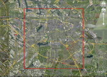
Figure 1. The area of Amsterdam for which the visibility of global landmarks was calculated (bounded by the red lines).
3. LANDMARK VISIBILITY ANALYSIS
Geographic Information Systems (GIS) provide a rich collection of analysis functionality for 2·5D models, such as visibility computation, which has been considerably researched already (e.g., Haverkort et al., Reference Haverkort, Toma and Zhuang2009; de Smith et al., Reference de Smith, Goodchild and Longley2012). For 3D analysis, however, only a few techniques have been established for general purposes. Moser et al. (Reference Moser, Albrecht and Kosar2010) presented an overview of current 3D GIS analysis capabilities for 3D city models. For example, although it is possible to add 3D features to the virtual environment in current GIS tools, visibility analysis is still performed solely on the 2·5D surface raster (e.g. Putra, Reference Putra2008; Vanhorn and Mosurinjohn, Reference Vanhorn and Mosurinjohn2010). 2·5D models, such as Digital Surface Models (DSM), are an extension of 2D representations by an additional attribute for the elevation, while in 3D models, elevation is the third dimension of every point in 3D space and thus part of the spatial structure.
Gross (Reference Gross1991) introduced an approach for analysing visibility by 3D perspective transformations. He coded the rendered objects by colour and counted the according pixels in the rendered image. Bishop et al. (Reference Bishop, Wherrett and Miller2000) additionally used depth images to classify objects in fore, middle, and background. Bishop (Reference Bishop2003) discussed these techniques, stating that these “have considerable benefit over the long standing 2·5D GIS approach”. Paliou et al. (Reference Paliou, Wheatley and Earl2011) utilized 3D modelling tools for 3D visibility analysis by adding light sources at possible observer points and calculating the illumination of target objects.
For the landmark visibility analysis we use an image-based 3D analysis technique (Engel and Döllner, Reference Engel and Döllner2009), which has several advantages over a GIS approach:
• The visual contact between surfaces can be quantified. Visibility is not handled in a binary manner (visible or not).
• The analysis is done in 3D and not on a 2·5D surface raster as in most GIS applications. In this way, general 3D spatial models can be used without restrictions regarding their geometry, topology and design.
• The quality of the models can be heterogeneous, not bound to the resolution of a raster or to other criteria e.g. specific levels of detail.
• The technique provides several parameters to adjust accuracy, computation time and memory consumption
3.1. Input and Output Data of the Algorithm
The visibility analysis is done in a pre-processing step. The input data for the algorithm is a virtual 3D city model with identified landmarks. The input models are not restricted to any particular format. The single requirement is that the model can be transformed into a triangle mesh.
The quality of the model is crucial for the analysis. This includes the position, size and form of the buildings and objects, but not their appearance, such as colours or textures. For our prototype we generated 3D building geometry from footprints, which corresponds to CityGML (Kolbe, Reference Kolbe, Lee and Zlatanova2009) LoD 1. More complex landmarks were modelled by multiple parts to create more correct building shapes and roof forms (corresponding to CityGML LoD 2).
The output of the algorithm is a digital raster image for every landmark, containing scalar values from 0 to 1 (Figure 2), which can be visualized as a terrain texture of the analysed area (Figure 3). Combined with a Digital Elevation Model (DEM), each pixel of the 2D image represents a 3D coordinate in the city model. The value at each pixel denotes the fraction of the landmark that is visible to a 1·75 m tall pedestrian located at these 3D coordinates. Thereby, 0 indicates that the landmark is totally invisible due to occlusion, 1 that the landmark is fully visible, and the values in between that the landmark is partially occluded. The distance to the landmark is not taken into account.
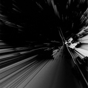
Figure 2. Visibility layer of the Rembrandt Tower in Amsterdam in the form of a grey scale raster image. Bright tints represent high visibility and dark ones represent low visibility.
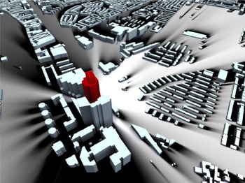
Figure 3. Visibility layer of the Rembrandt Tower in Amsterdam (red) – visualized as a terrain texture in the 3D city model. A Bright ground colour represents high visibility and dark represents low visibility.
3.2. Algorithm
Figuratively speaking, the discrete, image-based 3D analysis technique is based on traversing the analysed area and sending out rays from every point. Each of these rays evaluates whether it hits a landmark. To formalize the image-based 3D analysis, we introduce a function A that is evaluated for a position p in the virtual environment E:
 $${\bf A}(\,p,E) = \int_\Omega {\,f\,(\,p,hit(E,\omega ))} d\omega $$
In this definition, Ω denotes the scope of the analysis i.e. all the directions in which the rays can be sent out. The hit function determines the hit point that is hit by the ray ω and is closest to p. The evaluation function f evaluates the identity of the hit object and returns 1 if the object is a landmark, otherwise 0.
For a pragmatic, discrete implementation, we utilize the rasterization step of the programmable real-time rendering pipeline (Akenine-Möller et al., Reference Akenine-Möller, Haines and Hoffman2008) to determine the hit point and object instead of performing ray casting or ray tracing (Woop et al., Reference Woop, Schmittler and Slusallek2005). This way, we can easily exploit the computational capabilities of current consumer graphics hardware. Therefore, we place a virtual camera on p and render the virtual environment into G-buffers (Saito and Takahashi, Reference Saito and Takahashi1990), which are then analysed to calculate the results of f. G-Buffers are images containing additional information per pixel such as object identity. Thus, we approximate the scope Ω of the ray bundles by a 3D frustum of the camera and the hit function by z-buffering. This way, the analysis computation is performed on a discrete representation  $\rm \bar \Omega $ of all rays in Ω, that is a projection of the 3D scene at a sample point onto a finite, discrete view plane $\rm \bar \Omega = [0,N[ \times [0,M[$$. The implementation uses this view plane to compute an approximated, quantified result:
 $${\bf A}(\,p,E) \approx \int_{\rm \bar \Omega} {\,f\,(\,p,hil(E,\omega ))} d\omega = \sum\limits_{i \in [0,N} {\sum\limits_{[\,j \in [0,M} {\,f\,(\,p,hil(E,\omega _{i,j} ))}} $$
 By increasing or decreasing the resolution of $\rm \bar \Omega $ we can directly control the computational complexity and the approximation error of the analysis.
3.3. Implementation in Detail
To discretize the analysed area, the pixels of the output image are mapped to positions in the virtual 3D city model, which are translated to eye level above ground and used as the origin for a virtual camera. This camera is oriented to the current analysed landmark and represents a virtual pedestrian observing the landmark.
For every camera position, the landmark is rendered twice: firstly, solely to measure its size in pixels and thus its maximum visual quantity and secondly, together with the entire environment model. The second rendering of the landmark considers potential occlusions by the environment due to the depth test and the amount of rendered landmark pixels yields the actual visual quantity of the landmark. This is divided by the maximum visual quantity to get the relative visibility of the landmark.
Pixel counting can be accelerated using modern computer graphics hardware, by executing occlusion queries (Bartz et al., Reference Bartz, Meißner and Hüttner1998). Occlusion queries return the amount of fragments that pass all tests of the fragment pipeline. This saves the transfer of G-buffer from the graphics memory into the main memory, reducing computational time drastically. The implementation is based on OpenGL and the Virtual Rendering System (http://www.vrs3d.org).
3.4. Distortion Correction
Due to the perspective projection, pixels at the edges of the rendered G-Buffer cover a smaller solid angle than pixels in the centre. Therefore, objects projected on the edges of a G-Buffer appear larger than those in the centre; even if they have the same geometric size and distance to the virtual camera (Figure 4). To compensate for this distortion, we introduce a correction function e that weights the evaluation results:
 $${\bf A}(\,p,E) \approx \sum\limits_{i \in [0,N} {\sum\limits_{[\,j \in [0,M} {\,f\,(\,p,hit(E,\omega _{i,j} ))}} e(\omega _{i,j} )$$
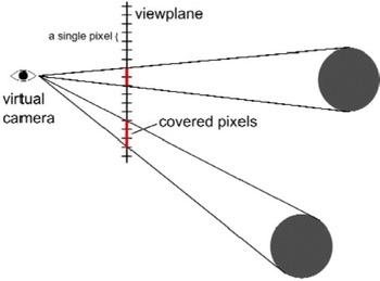
Figure 4. Objects projected on the edge of the view plane cover more pixels (in red) than objects of the same size and distance to the virtual camera but projected on the centre of the view plane.
The correction function e calculates for every pixel the viewing angle Δα in horizontal and vertical directions. The product of both is approximately the solid angle covered by the pixel (also called instantaneous field of view).
 $$\eqalign{e(\omega _{i,j} ) = & {\rm \Delta} \alpha _i {\rm \Delta} \alpha _j \cr {\rm \Delta} \alpha _i = & |atan(i - N/2 + 1) \cdot texelsize) - atan((i - N/2).texelsize| \cr texelsize = & \displaystyle{{{\rm tan}(\,fo\upsilon /2)} \over {N/2}}} $$
The results of e are pre-computed and stored in a texture with the same resolution as the viewport of the virtual camera. During G-Buffer processing, this value can be read and multiplied with the result of f.
3.5. Resolution of the Visibility Layer
The resolution of the discrete visibility layer has a high impact on the spatial accuracy during runtime of the application. Every pixel in the visibility layer stores the visibility of a landmark from a specific position. When the user is between these positions the visibility of the landmark has to be approximated by taking the nearest available position or by interpolating the values of the neighbouring positions. Near a building, these values can vary strongly (e.g., fully visible outside of the building and completely invisible for a position inside the building) and the approximation error for the values in-between can be large (Figure 5).
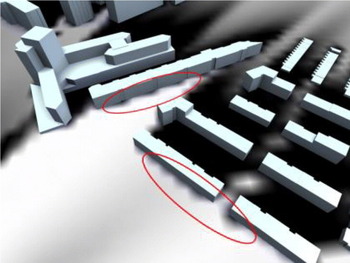
Figure 5. Interpolation errors using a visibility layer of insufficient resolution. Instead of hard transitions from visible to invisible under building walls, the interpolation of the visibility values for sparse camera positions inside and outside buildings creates a significant serrated area of incorrect partial visibility.
A higher resolution increases the density of virtual camera positions and reduces these approximation errors, but it also increases the computational time (Table 1), which is directly proportional to the amount of virtual camera positions. As the analysis is done as a pre-processing step, the memory consumption of the visibility layers is more crucial than the computational time. Memory is scarce on mobile devices and restricts the resolution for permanent storage.
Table 1. Analysis time and size of the resulting image per landmark as a function of the resolution. The analysis was performed on an Intel Xeon 2·8 GHz with 6 GB RAM and NVIDIA Quadro 4000.

4. MIGRATING TO MOBILE INTERFACES
To transform the results of the previously described framework to a landmark visibility indication function on an interface of a pedestrian navigation system, a prototype Android smartphone application was developed during the implementation stage of the UCD process. The prototype was named “LandNavin” (after Landmark-based Navigation interface), referred to as “LN” from now on. LN was built upon the Google Maps API, including, as basic tools, a zoom-able and pan-able map showing the position of the user, a scale bar, a rotating compass and different types of landmarks. Finally, it not only integrated the landmark visibility indication function, but also several new solutions for map orientation and control, routeing, landmark filtering, scaling and presentation, and concurrent provision of overview and detail maps. The implementation of these technical solutions was directed by the outcomes of the requirement analysis, conceptual modelling and solution design procedures performed earlier. However, the focus here is particularly on the presentation of the landmark visibility analysis framework and the usability of the landmark visibility indication as its result.
4.1. Computation and Performance
The computational power required for the 3D visibility analysis of the area of Amsterdam still exceeds the capabilities of modern mobile devices. As mentioned, a state of the art desktop computer needs about 6 minutes to compute a 512 × 512 pixel visibility raster map of a single landmark. A typical smartphone has limited CPU speed (e.g. 1 GHz), limited RAM memory (e.g. 512MB) and only a subset of the OpenGL specifications implemented in its graphics hardware. It is therefore not well-suited for the job. Hence, careful design was necessary from our side to provide an application that is suitable for smartphones, has comfortable performance, and still meets the requirements set onto the visualization aspects.
Several options were investigated, such as having the entire 3D visibility computation performed on the smartphone or on a desktop computer, having the computation performed on-the-fly (on-demand) or pre-calculated, and having the resulting visibility data available as a web service or in fixed images. Looking ahead, the performance and network bandwidth of the fastest mobile device available at the time of development (a Samsung Galaxy S i9000) was considered. After purchasing this device, extensive prototyping and testing was performed. What is technically achievable and what functionality is considered to work flawlessly (and add value to the usability) was then evaluated.
While the user is moving around, the application should provide him with live landmark visibility information. The device's GPS is used for the coordinates of his location, falling back to GSM cell-based positioning when the device fails to have a GPS lock. On-demand visibility analysis would make it easier to update the landmarks database, originally constituting a preferred situation. However, as noted earlier, this requires much more computational power and storage capacity than modern smartphones have available. Therefore, a client/server model was considered, with a powerful desktop server performing the on-demand 3D computations, and the smartphone receiving the result through a (wireless) network link/web service. The 3D visibility analysis of a single location with respect to a sole landmark is almost instantaneous (<2 ms on a modern desktop computer that could be used to host this as a web service). Nevertheless, the visibility requests would be almost continuous, as new visibility values per landmark are required whenever the user moves to a new position. Moreover, in our experience, the mobile network link has many hiccups or unexpected pauses, creating a bottleneck, possibly worsened by a concurrent use of the link for supplying the Google Maps base map raster data to the mobile application. Wi-Fi has fewer hiccups than 3G/GPRS connections, but cannot yet be used to walk around in a city (although many cities are now considering offering free Wi-Fi).
All things considered, a web service for the visibility data adds far too much latency to the mobile application, deteriorating its performance and response times, which become seconds instead of milliseconds, making it rather unusable. Therefore, we decided to follow the approach of pre-calculating 3D visibility for each landmark on a desktop computer and copying the resulting visibility images to the internal storage of the mobile device. Hence, as much as possible is pre-calculated and the remaining necessary calculations are kept to a minimum. Essentially, the only calculation still required by the mobile device is the application of the image's georeference formulae on the coordinates of the user's location to get the pixel location. Subsequently, the correct visibility value of that location can be immediately fetched from each image.
Tests have shown that, although the processing requirement is kept to a minimum, there is a limit to the number of landmarks that the application can handle comfortably (about 200). Above this number, more time is spent in processing the visibility values (adjusting each landmark icon on the map) rather than drawing the background map on the rotating canvas. This will be observed as a slowing-down response of the application's user interface, reducing its refresh rate to 1 frame per second or even less.
4.2. From Landmark Visibility to Landmark Icon
The visibility value of a landmark at a certain location indicates the fraction of visibility of that landmark from the user's location. To help users navigate better and understand faster their location and orientation, the following rules were applied for displaying landmark icons on the map of LN:
1 Landmarks behind the user (outside the user's field of view) are assumed to be invisible and their icon is not drawn on the mobile map.
2 Landmarks within the user's field of view are either fully visible, partially visible (fraction) or obstructed. Depending on the fraction of visibility, icons are drawn more intense/opaque: more visible landmarks can be drawn more intense/opaque and vice versa. Another option is to use different colours depending on landmark visibility, or a combination of transparency and colour.
Through experimentation, it appeared that the smartphone display is not well readable outdoors, due to the high intensity of ambient light. Thus icons should be clear and have a high contrast, while the transparency and gradient effects on colours should not be used. In our approach, the landmarks are either in the user's field of view (icon drawn) or behind the user (icon not drawn), and either visible (icon surrounded by a blue circle), or obstructed (icon surrounded by a red circle). A threshold is put on the visibility fraction, below which the landmark is regarded as obstructed, hence partially visible landmarks, with “too small” visible parts are “obstructed”.
The users are further assisted by the following tools to orient and locate themselves. First of all, the mobile device has an electronic compass, which permits drawing the map properly oriented. The map is centred to the user's location, indicated by a position arrow symbol. Landmarks behind the user (assuming the user is holding the mobile device top-side up) are not showing an icon on the map. All landmarks in front of the user are represented by an icon surrounded by a dashed coloured circle indicating landmark visibility (Figure 6).
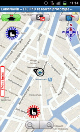
Figure 6. LN interface showing two global landmarks (churches). One is visible (blue dashed circle around landmark symbol) and the other is invisible (red dashed circle around landmark symbol) from the current position.
5. TESTING THE USABILITY OF THE LANDMARK VISIBILITY INDICATION
5.1 Methodology, participants and execution
Subsequent to the completion of LN, a field-based evaluation was executed to assess the usability of the prototype and its functions. The aim of the evaluation was to discover possible usability problems of LN and gather information on the performance and behaviour of TPs in a qualitative manner. This was done through a series of orientation and navigation assignments, as described in Section 2, with a moderate sample size, following well-established guidelines for usability testing studies.
Navigating from a starting point to an unfamiliar destination was the basis of each user test session incorporating a series of task scenarios that were developed. The scenarios reflected real use and user contexts in which there is a need for an electronic navigation tool. It was considered useful to compare the user's performance using another existing and comparable application interface next to LN, Google Mobile Maps (GM).
Conducting the usability testing in the field was regarded as more convenient than doing it in the lab, as central to this research were the links between reality, mobile maps and the users' mental maps. One of the main problems with field-based testing, the high-resource demand, was already successfully addressed by using the remote observation and recording system developed by Delikostidis and van Elzakker (Reference Delikostidis and van Elzakker2009a), extended by Delikostidis and van Elzakker (Reference Delikostidis and van Elzakker2011). The usability evaluation methodology was a combination of pre-selection questionnaires, observation, thinking aloud, synchronous multi-video and audio recording, screen logging, and post-session semi-structured interviews.
The pre-selection questionnaires were mainly used to check the (un-)familiarity of the TPs with the test areas but also profiled the TPs. Combining video observation and thinking aloud allowed for directly investigating TPs' reactions and interactions with the prototype and their feelings and mental processes while using LN (and GM) during the given tasks. And, finally, the post-session interviews helped to justify the experimental findings and also to gather more information on particular parts of the experiment where the TPs showed interesting or unexpected behaviour.
For this experiment, two test areas were selected. One was in the centre of Amsterdam, and the other one away from it, in a mostly residential and commercial area. The TPs were transported from Enschede (where recruited) to Amsterdam by train and instructed during the ride. Each TP executed a session in one of the two Amsterdam areas, divided into two parts. They had to navigate from a pre-defined starting point to the first destination using either LN or GM and then to navigate to the second destination using the other application interface. The sequence of using each interface was reversed for each new TP to control the “learning effect”. The total number of TPs was 24 (2 areas × 2 interface sequences × 6 TPs) and they represented potential users of the interface. Their age ranged from 18 to 60 years old and they had mixed profiles (16 with geo-information related backgrounds and eight without).
The research data acquired from the usability testing comprised of three types of material: questionnaires, synchronized video/audio recordings of the test sessions (Figure 7) and audio recordings of the interviews.
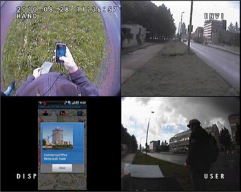
Figure 7. Example screenshot of the video recordings. The different cameras attached to the field observation and recording system have captured the interactions of the participants with the smartphone, the direction in which they look and a screenshot of the smartphone quantitative information from which the landmark visibility indication was evaluated and important usability issues were identified.
The first step in the analysis of the data was a verbatim transcription of the recordings with the qualitative research software Atlas.ti (http://www.atlasti.com). The transcription constituted a source of very rich and valuable qualitative and quantitative information from which the landmark visibility indication was evaluated and important usability issues were identified.
5.2 User test results
During the test tasks, the TPs made extended use of the landmark visibility indication, considering it an important supporting tool for their orientation and navigation. Using it, their performance was quite satisfying, leading to shorter average task completion times and higher task completion rates with LN compared to GM overall. Furthermore, the number of critical stops during navigation was lower with LN compared to GM in three out of four TP groups. The information acquired from the TPs through the post-session semi-structured interviews was also very helpful for assessing the usability of the landmark visibility indication. For the large majority of TPs (21 out of 24), this was a useful function, which could be further improved, according to a few TPs, by eliminating global landmarks from the map when not visible in reality. Among the TPs, only two found the function slightly confusing in the beginning and another three found its accuracy not always very good.
Although the landmark visibility indication did not work 100% accurately for all TPs and some of them did not experience it extensively in both states (visible/invisible), most of them found the function very useful. There were some suggestions for presentation modifications, but the majority of TPs liked the current implementation of the idea.
6. CONCLUSIONS
This paper has presented the theoretical framework of landmark visibility analysis, applied as a landmark visibility indication function in the development of LandNavin, a mobile navigation system for pedestrians. The algorithm used in the framework for landmark visibility analysis worked well and produced useful results. Although there are still issues to be addressed when migrating this technology to mobile devices, e.g. the difficulties of calculating landmark visibility for new landmarks dynamically on smartphones, its potential for creating very usable navigation systems is large.
Our LandNavin prototype, developed following a User-Centred Design methodology, was tested with representative users to evaluate the landmark visibility indication in real contexts of use. The aim of the assessment was to gather solely qualitative evidence on the usability of the method with a moderate number of participants.
The results show that a landmark visibility indication constitutes a useful tool for the majority of the participants, helping them relate reality with the mobile map more easily, which also supports the development and use of their cognitive maps. Most participants were satisfied with the implementation of the function, and the few who found it confusing or not always accurate, provided valuable feedback for further improvements. This should be taken into account when developing future iterations of the proposed approach.
Using landmark visibility analysis, different usable new tools can be developed for mobile navigation systems. User-centred design methodologies can help identify the real needs of users and design solutions to address them.


