


1. INTRODUCTION
Recently, Strap-down Inertial Navigation Systems (SINS) have demonstrated their value, finding applications in many fields, both military and civil, including aircraft, ships, cars and rocket systems. They employ an Inertial Measurement Unit (IMU) to measure acceleration with accelerometers and angular velocity with gyroscopes instead of using external information to determine position and attitude quickly and with relatively high accuracy. The initial alignment is a critical part of SINS operation, providing initial values, the purpose of which is to obtain a coordinate transformation matrix from body frame to computation frame, and drive the misalignment angles to zero. Several methods have been used to achieve the initial alignment. For example, gyrocompass alignment has been used (Kouba and Mason, Reference Kouba and Mason1962; Liu and Xu, Reference Liu and Xu2009; Hemmati and Masoumnia, Reference Hemmati and Masoumnia2012). The multi-position algorithm was applied in the fix-location alignment by Lai et al. (Reference Lai, Xiong, Liu and Jiang2012) and Liang et al. (Reference Liang, Yongyuan and Li2009). Also, the inertial freezing alignment (Liang et al., Reference Liang, Yongyuan and Wu2008) is an effective method to achieve fix-location initial alignment, which is faster while still maintaining a stronger anti-disturbance ability than some other methods. In this paper, our application is focused on a rocket navigation system. During the initial alignment, the rocket stands in a fixed location; however there are always disturbances such as wind gusts and wobble of the vehicle, causing a slight swaying of the rocket. The inertial freezing alignment is a perfect choice to accomplish the initial alignment in this situation.
The location of the IMU is not usually at the swaying centre, resulting in a lever arm effect (Xiasou and Dejun, Reference Xiaosu and Dejun1994) on the system, with a consequential impact on the initial alignment. Thus, lever arm effect introduces a large error in the output of the accelerometers, and analysis and removal of the lever arm disturbance is usually processed for the entire system in earlier works. However, in spite of the lever arm effect, the inertial sensors have constant drift and bias, which would generate rapid error accumulation or even divergence in the integration system. Here, sensor drift countered by lever arm effect compensation is proposed to improve navigation performance. Kalman filters (Fuquan et al., (Reference Fuquan, Chuanhong and Lianfeng2010); Titterton, (Reference Titterton2004); Ali and Ushaq, (Reference Ali and Ushaq2009); Hide et al., (Reference Hide., Moore. and Smith2003) and Pehlivanoglu and Ercan, (Reference Pehlivanoglu and Ercan2013)) have been widely used to compute the online estimation of sensor drift to achieve further compensation to improve alignment accuracy. In this paper, the harmful disturbing acceleration caused by lever arm effect is firstly filtered with a Finite Impulse Response (FIR) filter, and a rough attitude matrix is provided through inertial freezing alignment with the compensation of lever arm effect error. Next, a Kalman filter is employed to estimate sensor drift, and finally, the attitude matrix is calculated again with the compensation of the sensor drift and to get a more accurate mathematical platform for the initial alignment. A flowchart of the process is shown in Figure 1.
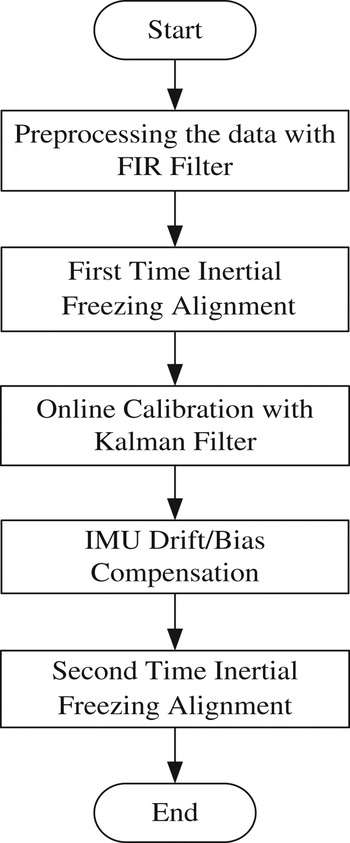
Figure 1. Flowchart of the initial alignment for the swaying base rocket navigation system.
The remainder of this paper is organized as follows: the description of inertial freezing alignment is presented in Section 2. The lever arm effect and its compensation are given in Section 3. Section 4 presents the analysis of inertial sensor drifts and bias to the system and Kalman filter online estimation. The algorithm verification experiments and conclusion can be found in Sections 5 and 6, respectively.
Assuming that L represents the latitude, λ represents longitude, ω ie is the Earth's rotation angular velocity, the local acceleration due to the actual gravity is denoted by g, ϕ is defined as the misalignment angle, (O bXbYbZb) stands for the body frame, (O eXeYeZe) is the earth frame, (O nXnYnZn) represents the navigation frame, (O iXiYiZi) is the inertial frame. Also, the inertial freezing frame i b0 is defined as fixing the vehicle frame at time t 0 to work as an inertial frame system afterwards. The subscripts b, e, i, n, i b0 denote the corresponding components in each frame.
2. PRINCIPLE OF INERTIAL FREEZING ALIGNMENT
The inertial freezing alignment is based on the principle that the movement trajectory of gravitational acceleration g is a conical surface in the inertial frame, and the movement of g includes the Earth's rotation axis information, with the projection of two different times' gravity g in the inertial frame. The attitude matrix can be computed with the analytical solution.
In this algorithm, the attitude matrix is broken down into four matrices:
 $$\eqalign{ & C_b^n = C_e^n C_i^e C_{i_{b0}} ^i C_b^{i_{b0}}$$
 $$ {\rm Where}\,{C_e^n\! = \!\left[ {\matrix{ { - \sin \lambda}\! &\! {\cos \lambda} \!&\! 0 \cr { - \sin L\cos \lambda}\! &\! { - \sin L\sin \lambda}\! &\! {\cos L} \cr {\cos L\cos \lambda}\! &\! {\cos L\sin \lambda}\! &\! {\sin L} \cr}} \right]_, C_i^e\! =\! \left[ {\matrix{ {\cos \omega _{ie} (t - t_0 )}\! &\! {\sin \omega _{ie} (t - t_0 )}\! &\! 0 \cr { - \sin \omega _{ie} (t - t_0 )} \!& \!{\cos \omega _{ie} (t - t_0 )}\! &\! 0 \cr 0 \!&\! 0 \!&\! 1 \cr}} \right]} $$ $C_b^{i_{b0}} $ is the transformation matrix from body b frame to inertial freezing frame i b0. This can be computed with the outputs of the gyroscopes through quaternion. Then, the key to obtaining the attitude matrix is the $C_i^{i_{b0}} $, it is completed by the following steps:
 $$f^{i_{b0}} = C_b^{i_{b0}} f^b = C_b^{ib0} ( - g^b + a_D^b + \nabla ^b ) = - C_i^{i_{b0}} g^i + C_b^{i_{b0}} (a_D^b + \nabla ^b )$$
Where a Db is acceleration disturbance, ∇b the acceleration bias. After integrating equation (2), while omitting the effect of periodic item a Db and small quantity ∇b, the velocity in the i b0 frame becomes
 $$V^{i_{b0}} = \int_{t_0} ^{t_k} {\,f^{i_{b0}}} dt = \int_{t_0} ^{t_k} {\left[ { - C_i^{i_{b0}} g^i + C_b^{i_{b0}} (a_D^b + \nabla ^b )} \right]} dt \approx \int_{t_0} ^{t_k} { - C_i^{i_{bo}} g^i dt} $$
Then we have  $\quad\tilde V^{i_{b0}} = \int _{t_0} ^{t_k} - C_i^{i_{b0}} g^i dt = C_i^{i_{b0}} \int _{t_0} ^{t_k} - g^i dt$
Let  $\int _{t_0} ^{t_k} - g^i dt$ be Vi, then
 $$V^i = \int_{t_0} ^{t_k} { - g^i} dt$$
Because
 $$g^i = C_e^i C_n^e g^n = \left[ {\matrix{ { - g \cdot \cos L \cdot \cos [\lambda + \omega _{ie} (t - t_0 )]} \cr { - g \cdot \cos L \cdot \sin [\lambda + \omega _{ie} (t - t_0 )]} \cr { - g\sin L} \cr}} \right]$$
Thus,
 $$\eqalign{ V^i (t_k ) =& \left[ {\displaystyle{{g\cos L \cdot [\sin (\lambda + \omega _{ie} (t_k - t_0 )) - \sin \lambda ]} \over {\omega _{ie}}}} \right. \cr & \times \left. {\displaystyle{{g\cos L \cdot [\cos \lambda - \cos (\lambda + \omega _{ie} (t_k - t_0 ))]} \over {\omega _{ie}}} g\sin L(t_k - t_0 )} \right]^T} $$
Assume two different times t k1,t k2, and t 0< t k1<t k2, using (3) and (4), we have
 $$\left\{ \matrix{\tilde V^{i_{b0}} (t_{k1} ) = C_i^{i_{bo}} V^i (t_{k1} ) \cr \tilde V^{i_{bo}} (t_{k2} ) = C_i^{i_{bo}} V^i (t_{k2} ) } \right.$$
So,
 $$\hat C_{i_{b0}} ^i = \left[ {\matrix{ {\left[ {V^i (t_{k1} )} \right]^T} \cr {\left[ {V^i (t_{k2} )} \right]^T} \cr {\left[ {V^i (t_{k1} ) \times V^i (t_{k2} )} \right]^T} \cr}} \right]^{ - 1} \left[ {\matrix{ {\left[ {\tilde V^{i_{b0}} (t_{k1} )} \right]^T} \cr {\left[ {\tilde V^{i_{b0}} (t_{k2} )} \right]^T} \cr {\left[ {\tilde V^{i_{b0}} (t_{k1} ) \times \tilde V^{i_{b0}} (t_{k2} )} \right]^T} \cr}} \right]$$
 Therefore,  $\hat C_{i_{b0}} ^i $ is derived from (7). Substituting it into (1), the attitude matrix can be computed.
3. PROCESSING AND COMPENSATION OF LEVER ARM EFFECT FOR ACCELEROMETERS
For the vehicle equipped with a strap-down inertial measurement unit, the ideal location of the accelerometers is in the swaying centre (O b), but they are usually sited elsewhere. Assuming that the accelerometers are located at P, and the vehicle body is swaying on its base, noise would be introduced in the outputs of the accelerometers, namely the centrifugal acceleration and tangential acceleration. This is known as the lever arm effect, as shown in Figure 2. Lever arm effect will seriously affect the accuracy of SINS in initial alignment (Xiaosu and Dejun, Reference Xiaosu and Dejun1994). There are several methods (Seo et al., (Reference Seo, Lee and Park2005), Yanrui et al. (Reference Yanrui, Deurloo and Luisa2011), Groves, (Reference Groves2003)) to compensate for the errors generated by the lever arm effect; in this paper, both parts of the lever arm effect have been analysed and compensated individually.

Figure 2. The principle of lever arm effect.
From Figure 2 we have
 $$R_p = R_o + r_p $$
Making derivatives to time in (8), we have
 $$f_p = f_o + \dot \omega _{ib} \times r_p + \omega _{ib} \times (\omega _{ib} \times r_p )$$
The disturbance acceleration resulting from lever arm effect can be divided into two parts, the centrifugal acceleration and tangential acceleration, and compensated separately.
• With the acknowledgement of the location of IMU installation and the swaying centre of the vehicle, according to (9), the centrifugal acceleration disturbance can be calculated from the outputs of gyroscopes and the length of lever arm in the three axis directions. This is then compensated from the output of accelerometers.
• As far as the tangential acceleration disturbance compensation is concerned, instead of using derivatives of gyroscope outputs and the lengths of lever arm based on (9), which would introduce great noise to the calculation and result in serious error, a FIR low-pass filter is adopted to pre-filter the acceleration. Since a FIR filter can effectively filter the tangential acceleration due to the vehicle linear movement, at the same time, it is possible to evaluate the time-delay of the FIR filter in order to compensate it to improve the accuracy of initial alignment.
The FIR digital filter is designed to use the limited length unit sample response h(n) to approximate the infinite length unit sample response h d(n) process. Window design is a commonly used method, and the main idea is to truncate the impulse response sequence h d(n) of an infinite time width with a window function sequence of a finite length in order to acquire the filter finite length impulse response h(n) of the FIR filter. As the unit sampling response h d(n) of the filter with the ideal rectangular frequency characteristics is symmetric, employing the symmetry window function sequence ω(n), h(n) would be accordingly symmetric, making the FIR digital filter H(ejω) in linear phase.
The window design method is described in Figure 3 as below:

Figure 3. The framework of window design.
In this paper, Kaiser Window, an adjustable window cluster, is adopted to design the FIR filter, whose expression is shown in equation (10):
 $$\omega (n) = \displaystyle{{I_0 [\beta \sqrt {\left. {1 - \left( {\displaystyle{{2N} \over {N - 1}} - 1} \right)^2} \right]}} \over {I_0 (\beta )}}0 \les n \les N - 1$$
Where, I 0(x) is the first class of zero-order Bessel function, expressed in series in equation (11). N is the length of the window and β is an adjustable parameter, which affects the side-lobe of the filter; the larger β is, the smaller the side-lobe of the spectrum will be. Usually, the value range of β is: 4 to 9.
 $$I_0 (x) = 1 + \sum\limits_{k = 1}^\infty {\left[\displaystyle{{\left(\displaystyle{x \over 2}\right)^k} \over {k!}}} \right]^2 $$
The steps for using Kaiser Window to design a linear-phase FIR filter are summarized as follows:
3.1. Window length calculation
The window length N is determined by the cut-off frequency of the pass-band ss, the attenuation frequency of the stop-band wp, and the sampling frequency.
 $$N = \displaystyle{A \over {\Delta \omega}} f_s $$
where A is a constant related to filters performance, normally set 10; f s is the sample frequency.
3.2. Calculating hd(n)
 $$h_d (n) = \displaystyle{1 \over {2\pi}} \int_{ - \pi} ^\pi {H_d} (e^{\,j\omega} )e^{\,j\omega n} d\omega $$
In most cases, it is too difficult to do the integral to H d(ejω) directly. So, we use M point sampling to H d(ejω).
3.3. Truncating hdp(n) to obtain h(n)
 $$h(n) = h_{dp} (n) \cdot \omega (n)$$
3.4. Obtaining the H(z) and H(ejω) of FIR from h(n)
After the FIR filter design is completed, it is inserted into the initial alignment system to remove the acceleration disturbance.
4. ESTIMATION AND COMPENSATION OF GYROSCOPE DRIFT
In addition to the lever arm effect, inertial sensor drift is another major factor that affects the system accuracy. To ensure initial alignment and navigation system accuracy, usually the IMU would be put onto a sophisticated turntable to complete calibration, and be compensated by the system software. Normally, after the completion of system calibration, gyros' and accelerometers' installation angles remain constant. However, non-repetitive errors in the gyro drift and accelerometer bias can occur with successive system starts, especially after a dormant period. The drift and bias would be very different relative to the original calibration value, as a result of which the system cannot meet the required accuracy of alignment and navigation. To solve this problem, the IMU should be disassembled from the vehicle and put on the turntable to re-calibrate gyro drift and accelerometer bias every few months in order to improve system performance. Obviously, this would be rather inconvenient in terms of utilization and maintenance. In this case, Kalman filtering is used to make an online estimation of the sensor drift rate to improve the alignment accuracy.
The continuous linear system state equation:
 $$\mathop X\limits^\cdot (t) = F(t)X(t) + \Gamma (t)W(t)$$
Observation equation
 $$Z(t) = H(t)X(t) + V(t)$$
Where, X(t) = [δV EδVN ϕE ϕN ϕU ∇x ∇yεx εy εz]T.
 $$F(t) = \left[ {\matrix{ {F_{11}} & {F_{12}} & 0 & { - f_u} & {\,f_n} & {C_{11}} & {C_{12}} & 0 & 0 & 0 \cr {F_{21}} & {F_{21}} & {\,f_u} & 0 & { - f_e} & {C_{21}} & {C_{22}} & 0 & 0 & 0 \cr 0 & { - \displaystyle{1 \over {R_n}}} & 0 & {F_{34}} & {F_{35}} & 0 & 0 & { - C_{11}} & { - C_{12}} & { - C_{13}} \cr {\displaystyle{1 \over {R_e}}} & 0 & {F_{43}} & 0 & { - \displaystyle{{V_n} \over {R_n}}} & 0 & 0 & { - C_{21}} & { - C_{22}} & { - C_{23}} \cr {\displaystyle{{tgL} \over {R_e}}} & 0 & {F_{53}} & {\displaystyle{{V_n} \over {R_n}}} & 0 & 0 & 0 & { - C_{31}} & { - C_{32}} & { - C_{33}} \cr 0 & 0 & 0 & 0 & 0 & 0 & 0 & 0 & 0 & 0 \cr 0 & 0 & 0 & 0 & 0 & 0 & 0 & 0 & 0 & 0 \cr 0 & 0 & 0 & 0 & 0 & 0 & 0 & 0 & 0 & 0 \cr 0 & 0 & 0 & 0 & 0 & 0 & 0 & 0 & 0 & 0 \cr 0 & 0 & 0 & 0 & 0 & 0 & 0 & 0 & 0 & 0 \cr}} \right]$$
 $$\eqalign{ & F_{11} = \displaystyle{{V_n} \over {R_n}} {\rm t}gL - \displaystyle{{V_u} \over {R_n}}, \;F_{12} = 2\omega _{ie} \sin L + \displaystyle{{V_e} \over {R_e}} {\rm t}gL,\;F_{22} = - \displaystyle{{V_u} \over {R_n}}, \cr & F_{21} = - 2(\omega _{ie} \sin L + \displaystyle{{V_e} \over {R_e}} {\rm t}gL),\;F_{34} = \omega _{ie} \sin L + \displaystyle{{V_e} \over {R_e}} {\rm t}gL, \cr & F_{35} = - (\omega _{ie} \cos L + \displaystyle{{V_e} \over {R_e}}), \;F_{43} = - F_{34}, \;F_{53} = - F_{35}} $$
C 11∼C 33 are the elements of the attitude matrix. A local level ENU (East-North-Up) frame is adopted as the navigation frame. Subscripts x, y, z denote the body frame axes. V, δV and ϕ represent the velocity, velocity error and attitude error, respectively. f is the output of the accelerometer. ∇ x ,∇y are generalized accelerometer errors, ε is gyro drift.
In the simulation, the system needs to be discretized, the discrete system state equation and observation equation shown in (17) and (18).
 $$X_k = \phi _{k,k - 1} X_{k - 1} + \Gamma _{k,k - 1} W_{k - 1} $$
 $$Z_k = H_k X_k + V_k $$
The system noise is W k=[w vewvn wϕe wϕn wϕu 0 0 0 0 0]T
The measurement equation is:
 $$Z_k = \left[ {\matrix{ {V_{se} + v_{noise}} \cr {V_{sn} + v_{noise}} \cr}} \right] = H_k X + V_k $$
 Where, H k is the measurement matrix, V se, Vsn are eastern velocity error and the northern velocity error,  $H_k = \left[ {\matrix{ 1 & 0 & 0 & 0 & 0 & 0 & 0 & 0 & 0 & 0 \cr 0 & 1 & 0 & 0 & 0 & 0 & 0 & 0 & 0 & 0 \cr}} \right]$, v noise is the velocity noise, V k is the system measurement noise.
The specific steps of a discrete Kalman filter are as follows:
State forecast equation:
 $$\hat X_{k,k - 1} = \Phi _{k,k - 1} \hat X_{k - 1} $$
State estimation:
 $$\hat X_k = \hat X_{k,k - 1} + K_k [Z_k - H_k \hat X_{k,k - 1} ]$$
Filter gain matrix:
 $$K_k = P_{k,k - 1} H_k^T [H_k P_{k,k - 1} H_k^T + R_k ]^{ - 1} $
Prediction error variance matrix:
 $$P_{k,k - 1} = \Phi _{k,k - 1} P_{k - 1} \Phi _{k,k - 1}^T + \Gamma _{k,k - 1} Q_{k - 1} \Gamma _{k,k - 1}^T $$
Estimation error variance matrix:
 $$P_k = [I - k_k H_k ]P_{k,k - 1} [I - K_k H_k ]^T + K_k R_k K_k^T $$
Where X k is the system n-dimensional estimated state vector at time k. Φk,k−1 is the system n×n dimension state transition matrix from time k−1 to time k, W k−1 is the p-dimensional system noise sequence at the time k−1, Γk,k−1 is the n×p dimension noise input matrix, indicating the impact level of system noise on each state from time k−1 to time k. Z k is the system m-dimension observation sequence at time k, V k is the m-dimension observation noise sequence, H k is the m×n dimension observation matrix. Q k is the p×p dimension symmetric non-negative definite covariance matrix of the system process noise W k, Rk is the m×m dimension positive definite covariance matrix of the system measurement noise V k.
5. EXPERIMENTS AND VALIDATION
A block diagram describing the algorithms involved to obtain better accuracy for the rocket initial alignment system is in Figure 4.

Figure 4. The framework of the improved initial alignment method.
During the simulations, the outputs of the gyros and accelerometers are simulated to provide the raw data, the lever arm disturbance is processed with the FIR filter and the gyro drift is estimated and compensated by the Kalman filter. The algorithm has been tested and validated by means of simulations on the platform of VC++. Considering that the algorithm is applied in the rocket navigation system, the corresponding simulation setting is presented here as follows:
Assuming that the vehicle is on the swaying base, the azimuth swaying amplitude is 0·3°(swaying cycle is 7 s), the rolling swaying amplitude is 0·15°(swaying cycle is 6 s), the pitch swaying amplitude is 0·1°(swaying cycle is 5 s). The initial position is 32°N, 118°E.
The gyro constant drift rate ε x=ε y=ε z=0·01°/h, and the accelerometer bias is ∇ x=∇ y=∇ z=0·01×10−3g. The stochastic noise of the SINS gyroscopes and accelerometers is Gaussian white noise with the level of N(0,(0·005°/h)2) and N(0, (0·05×10−3 g)2), respectively. r x=0·7 m, r y=0·7 m, r z=40·0 m.
Figure 5 shows the estimation of gyro drifts in three axes with the Kalman filter. It can be seen that the gyro's drift in x direction and y direction are estimated in 12 min, while the drift in z direction is not capable of estimation due to its low observability (Andrews et al., (2007), Xianghong and Dejun, (Reference Xianghong and Dejun1997)) on a swaying base. These estimated gyro drifts are capable of being compensated in the following section to improve system performance.

Figure 5. Gyro drift estimations in three axes.
Figure 6 shows the 30 s acceleration signals in three axes before and after FIR filtering. The red dashed line is the acceleration signal before the filter and the blue curve is the acceleration signal after the FIR filter. It can be clearly seen that the disturbance on the acceleration signals are greatly filtered by the FIR filter, which helps to ensure the success of the initial alignment.
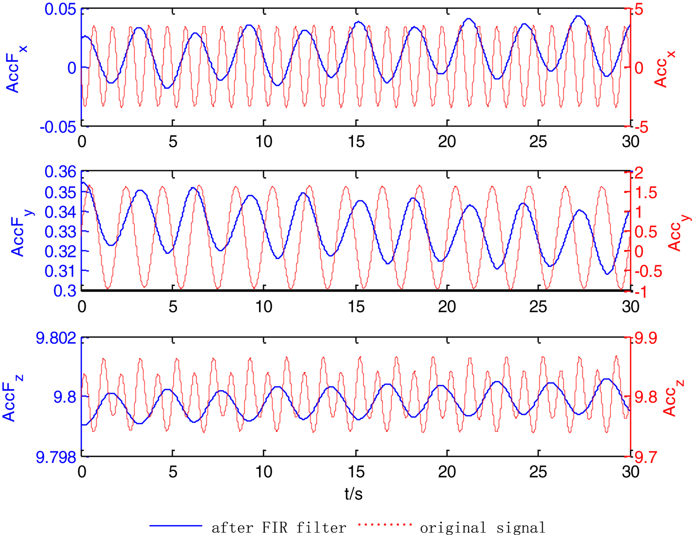
Figure 6. Accelerations in three axes before and after FIR filtering.
Figures 7–9 show eight times attitude error with different compensation levels. Figure 7 shows the azimuth error, Figure 8 shows the pitch error and Figure 9 shows the roll error. It is clear that attitude accuracy has been greatly enhanced after lever arm effect compensation, and with subsequent gyro drift compensation, the alignment is at least 6–8 times more accurate. This illustrates the effectiveness of the algorithm.

Figure 7. Eight times azimuth error with different compensations.

Figure 8. Eight times pitch error with different compensations.

Figure 9. Eight times roll error with different compensations.
6. CONCLUSION
This paper presents an efficient alignment approach for a swaying base rocket navigation system. An algorithm associated with the inertial freezing alignment is employed to obtain the mathematical platform for the navigation system. Considering the environmental disturbance and the sensor drift as the main error source, an FIR filter has been applied to the system to reduce the lever arm effect on the acceleration measurement. In addition, a Kalman filter is implemented to compute the online estimation of gyro drift that can be compensated to improve the system performance. Experiments were conducted and the results are so encouraging that the inertial freezing alignment with the FIR and Kalman filters is able to provide a viable means of achieving good accuracy for the rocket initial alignment system. To verify its true robustness, further research in laboratory and even field tests would be needed. Moreover, it will be necessary to examine more data records corresponding to a wider range of operational and environmental cases.
ACKNOWLEDGMENTS
This work is funded by The Major State Basic Research Development Program of China (973 program, No.613121010201) and the Scientific Research Foundation of Graduate School of Southeast University with Granted number (YBJJ1242).


