


Introduction
Within the framework of the European Project for Ice Coring in Antarctica (EPICA) a deep ice core (EDML) was drilled in Dronning Maud Land (DML), Antarctica, near the German summer station, Kohnen (EPICA Community Members, 2006). To obtain high-resolution climate information of the last glacial cycle, a drilling site was chosen that provides comparatively high accumulation rates, large ice thickness and nearly undisturbed layering of the ice. The EDML drilling site (75.0025° S, 0.0684° E;2891.7m above the World Geodetic System 1984 (WGS84) ellipsoid) is located in the Atlantic sector of Antarctica (Fig. 1) and is used to investigate the connection between Northern and Southern Hemisphere climate variability in the past. The area surrounding the EDML drilling site is situated between two transient ice divides which fork at approximately 75.1° S, 1° E, according to the elevation model of Reference Bamber and BindschadlerBamber and Bindschadler (1997). The deep ice-core drilling was carried out in the austral summer seasons 2000/01 to 2005/06. The ice thickness in this region is 2782 ± 5 m, as measured by airborne radio-echo sounding, and the total recovered core length was 2774.15 m (personal communication from F. Wilhelms, 2006). The drilling finished when subglacial water entered the borehole. The recent accumulation rate in the surroundings of the EDML drilling site is 64kgm–2 a–1(Reference Eisen, Rack, Nixdorf and WilhelmsEisen and others, 2005), with small-scale spatial variability of ~10%.
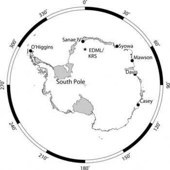
Fig. 1. Location map of the EDML drilling site in Antarctica, marked with a star. Six International Global Navigation Satellite Systems Service (IGS) reference stations are indicated with filled circles. They were used for determining the position of the local reference point Kohnen Reference Station (KRS) adjacent to the EDML drilling site.
Accurate interpretation of the EDML ice-core data (e.g. past accumulation from annual layer thicknesses) requires knowledge of the complete strain field to correct for dynamic layer thickness variation. In this paper, we determine the topography, flow and strain field in the wider surroundings of the drilling site. Similar investigations were previously made at several drilling sites in Antarctica and Greenland. For example, Reference VittuariVittuari and others (2004) present a velocity field at Dome C (the first EPICA deep-drilling site (EPICA Community Members, 2004)) in the Indo-Pacific sector of the Antarctic ice sheet. In Greenland, Reference Hvidberg, Keller and GundestrupHvidberg and others (2002) investigated the ice flow at NorthGRIP, a drilling site that is also located in the vicinity of a transient ice divide. For the EDML site, a digital elevation model (DEM) is derived from the combination of ground-based kinematic GPS (global positioning system) and ICESat (Ice, Cloud and land Elevation Satellite) laser altimetry, providing highly accurate surface topography in the region of interest. This forms, together with ice velocity data, the basis for estimating and interpreting deformation in the upper part of the ice sheet.
Data and Methods
Static and kinematic GPS measurements were used for our investigation. The elevation data derived from the kinematic GPS data were complemented by NASA’s ICESat satellite laser altimetry data (US National Snow and Ice Data Center (NSIDC) http://nsidc.org/data/icesat/).
Kohnen Reference Station (KRS)
Kohnen Reference Station (KRS), which is located at the German summer station Kohnen (75.0018° S, 0.0667° E), is used for processing our GPS measurements. This is a nonpermanent GPS station, providing data at 1 s intervals only during the drilling campaigns 2000/01 to 2005/06 (with interruptions in the season 2004/05). The KRS GPS antenna was mounted on the northern corner of the Kohnen station. With the aid of the International Global Navigation Satellite Systems Service (IGS) network, the daily position of KRS was determined using the GPS stations Mawson, Sanae IV, Syowa, Davis, Casey and O’Higgins (Fig. 1). The KRS positions were determined with the post-processing software GAMIT, assuming motion of the site was negligible during the processing window (Scripps Institution of Oceanography, http://sopac.ucsd.edu/processing/gamit/).
Surface profiles from kinematic GPS measurements
Kinematic GPS measurements combined with ground-penetrating radar (GPR) recorded during the 2000/01 field campaign (Reference Eisen, Rack, Nixdorf and WilhelmsEisen and others, 2005) form the basis for generating a DEM with a higher accuracy and resolution than former DEMs in the surroundings of the EDML drilling site. A Trimble SSI 4000 GPS receiver was mounted on a snowmobile which was navigated at a velocity of about 10kmh–1 along predefined tracks (Fig. 2, solid lines) in the area of investigation (74.8–75.1 ° S, 0.2° W–0.8° E). There are two networks of kinematic GPS profiles, both centered on the EDML drilling site. The length of the edges of the first grid is 10 km with a profile spacing of 1–3 km. The second grid is a star-like pattern, which consists of seven 20–25 km legs. The kinematic GPS data were processed with Trimble Geomatics Office™ (TGOTM), including precise ephemeris and ionosphere-free solution.

Fig. 2. Data coverage for the DEM derived in the present study. The solid lines present the kinematic GPS profiles, and the dotted lines the ICESat GLAS12 ground tracks. Sites used for static GPS measurements are marked with filled circles; the star marks the EDML drilling site.
Flow and strain networks using static GPS measurements
In order to determine horizontal velocities and strain rates, static GPS measurements around the EDML drilling site were carried out with Ashtech Z-12 and Trimble SSI 4000 GPS receivers in the austral summer seasons between 1999/2000 and 2005/06. For the velocity network 13 points in the surroundings of the EDML drilling site were used (Fig. 2). These points are marked with aluminium stakes and were surveyed for approximately 1 hour per season to find their positions. The static GPS data were also processed with TGOTM. All determined positions are available in the PANGAEA database (doi: 10.1594/PANGAEA.611331).
Surface profiles from satellite altimetry
The Geoscience Laser Altimeter System (GLAS) on board NASA’s ICESat provides global altimetry data with a wavelength of 1064 nm up to 86° N and 86° S. The laser footprint has a diameter of 60 m, and the along-track distance between the footprints is 172 m. The positioning error is 35 m (Reference ZwallyZwally and others, 2002). In this paper, GLAS12 altimetry data for the periods L1a (20 February to 20 March 2003) and L2a (25 September to 18 November 2003) are used to determine the surface elevation model of the investigated area. The ground tracks of these measurements across the investigated area are plotted in Figure 2 as dotted lines. The GLAS12 satellite laser altimetry data and the corresponding NSIDC GLAS Altimetry elevation extractor Tool (NGAT) are provided by NSIDC (http://nsidc.org/data/icesat/).
Data Accuracy
Knowledge of potential errors is essential for determining the quality of the kinematic and static GPS data. The general GPS errors and those of our solutions are presented in this section. The distance between the reference station and the survey point or profile is the principal factor affecting the accuracy of the position to be determined.
GPS errors
GPS observations at high latitudes are affected by the relatively weak satellite geometry, and hence formal errors are larger here than at other latitudes. Ionospheric and tropospheric effects were minimized by adopting the ionosphere-free linear combination and applying a tropospheric model. Further error reduction occurs through the double-differencing approach used in TGOTM and the relatively short baselines.
Kinematic GPS measurements
Since we used KRS, located in the center of the kinematic GPS profiles, systematic positioning errors are negligible. The accuracy of the kinematic GPS measurements is estimated by a crossover-point analysis. The histogram in Figure 3 shows the elevation differences at the 1615 crossover points. The mean elevation difference is 0.03 m with a standard deviation of 0.12 m.

Fig. 3. Histogram of elevation differences at 1615 crossover points of the surveyed kinematic GPS profiles.
Static GPS measurements
All stakes (Fig. 2) were occupied for an observation period of ~1 hour in several campaigns. The length of the baselines to KRS varied between 0.03 km (BA01) and 19.4 km (DML27). The positions of all stakes were computed using TGOTM, and the formal horizontal and vertical errors (Table 1) were derived for every point in a processing report. The formal errors issued by GPS software are usually over-optimistic. Experience shows that these errors need to be scaled by a factor of 5–20, to be closer to the true uncertainty of the static GPS (personal communication from M. King, 2007). We take a factor of 20 as a conservative estimate of the precision of the GPS positions. As the accuracy depends on the baseline length, we use the points BA01 and DML27 to estimate the accuracy of the static GPS measurements.
Table 1. Table 1. Error estimates for BA01 and DML27
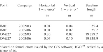
The positions of these two points were calculated against KRS for two campaigns. They have quite different horizontal and vertical errors, which can be attributed to the longer baseline length between KRS and DML27. However, there are also significant differences between campaigns for the same point. For DML27, the horizontal and vertical errors in 2002/03 are almost an order of magnitude larger than in 2005/06. This may stem from the high sunspot activity in 2002/03 (http://solarscience.msfc.nasa.gov/SunspotCycle. shtml) in combination with the baseline length, despite using the ionosphere-free solution of TGOTM. We assume that the maximum horizontal and vertical errors for our solutions are given by the values for DML27 of 0.30 m and 0.82 m, respectively, from the campaign in 2002/03.
GLAS data
ICESat’s positioning precision is stated as 35 m and the predicted elevation data accuracy is 0.15 m (Reference ZwallyZwally and others, 2002). Reference ShumanShuman and others (2006) presented a new elevation accuracy assessment of ~0.02 m for low-slope and clear-sky conditions. Our area of investigation is a low-slope region, but clouds during the observation period cannot be excluded over the whole period. The elevation measurements of the ICESat laser altimeter refer to the TOPEX/ Poseidon ellipsoid. Differences in elevation between the TOPEX/Poseidon ellipsoid and the WGS84 ellipsoid are approximately 0.71 m in the region of interest (personal communication from T. Haran, 2005). When transforming to the WGS84 ellipsoid we subtract this value from all GLAS12 elevation data.
Results
Surface topography
The derived surface topography in the area of investigation refers to the WGS84 ellipsoid and is a combination of the GPS and the GLAS12 datasets (Fig. 4, contours). A crossover-point analysis was performed before combining the datasets to identify systematic offsets and to estimate the uncertainties. As crossover points for the GPS data we use the average of all GPS measurements within the diameter of the GLAS footprint of about 60 m. Considering all crossover points, the GLAS12 data (transformed to the WGS84 ellipsoid) are found to be 0.119 m lower than the GPS data, on average. This elevation difference was added to the GLAS12 data, i.e. we corrected the elevations to the GPS profiles. To get sufficient spatial coverage of elevation data over the whole area of investigation, we interpolated the combined dataset with a minimum-curvature algorithm (Reference Wessel and SmithWessel and Smith, 1991) on a 5 km × 5 km grid (Fig. 4). With this grid size, at least one data point was available for each gridcell, even several tens of kilometers away from the drilling site.
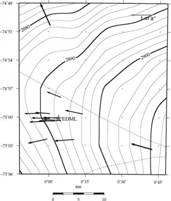
Fig. 4. Surface flow-velocity vectors in the area of interest, plotted on the contour map of the combined and gridded (5km × 5 km) GPS/GLAS12 elevation model. The contour interval is 2m. The dotted curves indicate the ice divide corresponding to the DEM of Reference Bamber and BindschadlerBamber and Bindschadler (1997).
Surface velocity
The velocity magnitude at the survey points between the two ice divides varies between 0.62 m a–1 (PEN5) and 0.96 m a–1(DML27). The flow direction varies between 257.9° (PEN4) and 291.3° (PEN1). The flow velocity of DML26, north of the divide, is outside this range, moving in a direction of 335.9° with a magnitude of 1.07 m a–1 (Table 2; Fig. 4).
Table 2. Calculated mean annual horizontal ice-flow velocities
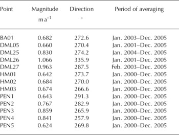
The location of the EDML drilling site was surveyed on 10 January 2001, before the drilling operation started, yielding 75.0025° S, 0.068° E and 2891.7 m at the snow surface. As excavation of the drill trench does not allow accurate remeasurements, we use the mean velocities of the points next to it, DML25 and BA01. We thus obtain a value of 0.756m a–1 in the direction of 273.4° for the ice velocity at the drilling site. The precision of the velocity measurements differs, depending on the period and data used (see Table 1). We therefore perform a propagation of errors by
Only the horizontal errors are used; the vertical errors are neglected for calculating the propagated error (δv) of the annual movement. Here, v is the velocity magnitude and s the horizontal offset of the survey point over the measurement interval (t). The term δsm is the mean of the horizontal errors for the survey point of the two campaigns used for the determination of the velocities. The time error, δt, is assumed to be a constant of 1 day (1/365.25 years), because the start and end time is rounded by the day. The resulting errors for sites DML27 and BA01 are 0.059 and 0.003 m a–1, respectively. As discussed above, we take the error at DML27 as the maximum error of the velocity determination, as it has the longest baseline.
Surface strain rates
Strain rates were determined from a pentagon-shaped network (PEN1–PEN5) with BA01 as the center reference pole (Fig. 5). Using the horizontal surface velocities in Table 2, with the geodetical nomenclature of y as the eastward and x as the northward components, we determine the strain-rate components from (Reference PatersonPaterson, 1994)
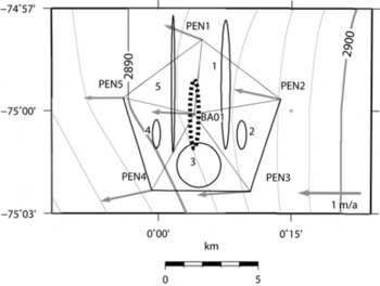
Fig. 5. Velocity vectors of the pentagon-shaped network (PEN1–PEN5) and BA01. Strain ellipses are plotted for the five strain triangles, indicated by numbers 1–5. The mean strain ellipse (dotted) is centered on BA01. See text for the calculation of the mean strain ellipse. The elevation contour interval is 2m.
and the combined strain rate as
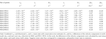
where Δvx and Δvy are the differences of the x and y velocity components of the considered pair of survey points, and ∆x and ∆y are the distances between the stakes in the × and y directions. Distances from the reference pole to each pentagon point vary between 3961.85 m (BA01–PEN5) and 5173.28 m (BA01–PEN3). Using Equation (3) the combined surface strain rate is calculated for every pair of neighboring points (west–east and south–north), yielding ten values (Table 3).
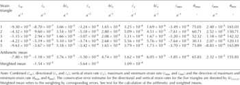
Table 3. Strain rates for pairs of survey points
To determine the strain rates, we divide the pentagon into five strain triangles (Fig. 5) and assume the strain is constant over the area of the triangle. We calculate the average of the strain for each triangle (e.g. the mean of BA01/PEN1, BA01/ PEN2 and PEN1/PEN2 for the northeastern triangle, numbered 1). The principal components are calculated using the rotation, θ, of the × and y axes
This provides one of two values for θ, which are 90° apart. One gives the direction of the maximum strain rate, ![]() max, the other of minimum strain rate,
max, the other of minimum strain rate, ![]() min. The strain-rate magnitudes along these directions follow from
min. The strain-rate magnitudes along these directions follow from
This calculation is repeated for every strain triangle. The direction of maximum strain rate varies between 30.1° and 75.0°. Using the incompressibility condition (Reference PatersonPaterson, 1994)
we estimate the flow-induced vertical strain rate ![]() z
. It varies between 1.31 × 10⁻⁶ and 3.79 × 10⁻⁴a–1 (Table 4), with a standard variation of 6.49 × 10⁻⁵ a–1. To estimate a strain rate representative of the EDML drilling site, we determine the average horizontal deformation and its direction at BA01. For this purpose, the arithmetic means of
z
. It varies between 1.31 × 10⁻⁶ and 3.79 × 10⁻⁴a–1 (Table 4), with a standard variation of 6.49 × 10⁻⁵ a–1. To estimate a strain rate representative of the EDML drilling site, we determine the average horizontal deformation and its direction at BA01. For this purpose, the arithmetic means of ![]() xy
,
xy
, ![]() x
and
x
and
![]() y
from the strain triangles are calculated and used in Equations (4) and (5) (Table 4). The maximum rate is –1.85 × 10⁻⁴a–1, acting in the direction of 65.8°. The minimum rate, 2.32 × 10⁻⁵a–1, acts in the direction of 155.8°. In addition to the arithmetic mean, we determine the weighted mean for the directional and vertical strain-rate components (
y
from the strain triangles are calculated and used in Equations (4) and (5) (Table 4). The maximum rate is –1.85 × 10⁻⁴a–1, acting in the direction of 65.8°. The minimum rate, 2.32 × 10⁻⁵a–1, acts in the direction of 155.8°. In addition to the arithmetic mean, we determine the weighted mean for the directional and vertical strain-rate components (![]() x,y,z), using the strain-rate error weights (Table 4). The arithmetic mean of the vertical strain rate,
x,y,z), using the strain-rate error weights (Table 4). The arithmetic mean of the vertical strain rate,
![]() z, is (1.62 ± 1.25) × 10–4 a–1, and the weighted mean is (1.09 ± 1.25) × 10–4 a–1.
z, is (1.62 ± 1.25) × 10–4 a–1, and the weighted mean is (1.09 ± 1.25) × 10–4 a–1.
Table 4. Strain rates for the strain triangles
Discussion
The DEM presented here is compared with the DEM generated by Reference Bamber and BindschadlerBamber and Bindschadler (1997) from European Remote-sensing Satellite-1 (ERS-1) radar altimetry, which is also available on a 5 km × 5 km grid. For comparison, we subtract the Reference Bamber and BindschadlerBamber and Bindschadler (1997) DEM from our combined GPS/GLAS12 DEM. The northeastern edge of the area of investigation is striking, where the elevations of the Reference Bamber and BindschadlerBamber and Bindschadler (1997) DEM are about 2 m higher than those in our DEM (Fig. 6). Calculating the mean difference between the combined GPS/GLAS12 DEM and the Bamber and Bindschadler (1997) DEM for every 5 km × 5 km gridcell, we determine a mean elevation difference of –0.33 m. That is, the DEM of Reference Bamber and BindschadlerBamber and Bindschadler (1997) is about 0.3 m higher than our combined GPS/GLAS12 DEM.
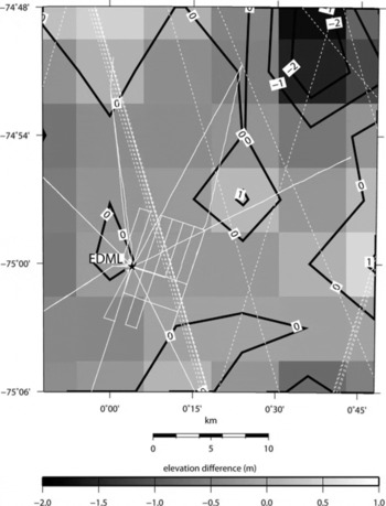
Fig. 6. Elevation differences of our GPS/GLAS12 DEM minus the Reference Bamber and BindschadlerBamber and Bindschadler (1997) DEM. The contour interval is 1 m. Kinematic GPS and GLAS12 data coverage used in this paper (Fig. 2) are plotted as white dotted (GLAS12) and solid (GPS) lines.
The topography in the region of interest shows a smooth surface, slightly sloping down to the west. One major feature is a transient ice divide, which splits ~20 km upstream of the drilling location, thus separating three drainage basins. Of our 13 survey points, 12 are located between the two branches of the ice divide;only DML26 is located north of both ice branches (Fig. 4). As it represents a different drainage basin and flow regime, we exclude DML26 from further analysis. The ice divide and the local surface elevation are the largest factors determining the flow and strain field. This is evident from comparison of the mean slope direction at the drilling site with the mean flow direction of 273.5° from the GPS-based velocity measurements. Small differences in magnitude and direction of the horizontal ice-flow velocities of the survey points are likewise mainly caused by the relative location of the survey point in respect to the ice divide. Points very close to the ice divide are generally slower and the direction of movement is nearly parallel to the course of the divide (Fig. 4 and Table 2, e.g. PEN1). The magnitude of the flow velocity increases with increasing distance from the divide, and the northward flow component is reduced (Fig. 4;Table 2). An exception is PEN5, which has a slightly lower velocity (0.624 m a–1) than PEN1 (0.643 m a–1) despite the greater distance from the divide. Although this difference is smaller than the estimated conservative maximum velocity error of 0.059 m a–1, we try to identify the origin of this variation.
Investigating the local bedrock topography in the vicinity of PEN5, available from airborne radio-echo soundings (Reference Steinhage, Nixdorf, Meyer and MillerSteinhage and others, 1999), PEN5 is found to be located above a depression of the subglacial topography (Fig. 7). The depression is ~5 km wide and several tens of meters deep, with respect to the surrounding average bedrock elevation. Because of the smoothing effect of ice dynamics, the surface elevation is much smoother than the bedrock topography. Surface topography varies only in the order of meters. The depression therefore simply causes locally increased ice thickness, but not a significant feature at the surface. The slightly lower velocity at PEN5, compared to the other stakes, is thus a consequence of the flux balance required by the larger ice thickness.

Fig. 7. Subglacial topography of the area of investigation gridded on a 500m × 500m raster after Reference Steinhage, Nixdorf, Meyer and MillerSteinhage and others (1999). The spacing between the contours is 50 m. The dotted line represents the ice divide corresponding to Reference Bamber and BindschadlerBamber and Bindschadler (1997).
The surface strain rate at BA01, averaged from the strain triangles of the five pentagon points (PEN1–PEN5), is considered to be representative for the EDML ice core, as BA01 is only 93 m to the northeast of the drilling site. Most error estimates for the strain rates (Tables 3 and 4) are about equal to or smaller than the nominal value of the strain rate. For some strain rates with very small nominal values, the error is more than one order of magnitude larger (e.g. triangle 3, Table 4). We emphasize that the velocity errors are very conservative estimates, so the strain-rate errors are also conservative estimates. The average maximum principal component of the strain rate at BA01 is negative (–1.85 × 10⁻⁴a–1). It acts as a compressing force in the direction of 65.8°. The minimum principal component of the strain rate at BA01 is positive (2.32 × 10⁻⁵a–1). It therefore corresponds to a dilatational force and acts along an axis in the direction of 155.8°. This results from the low magnitude of the velocity at PEN5. Both BA01 and PEN2 (upstream of PEN5) are moving faster than PEN5, which induces the along-flow compression of the ice mass. The average vertical strain rate, as calculated above, shows that the compression in the northwest–southeast direction only partly compensates the dilatational component of the strain field in the northeast– southwest direction, perpendicular to the ice flow at EDML, and layer thinning is required in the vertical component to achieve balance.
Conclusion
We provide an improved dataset for the surface topography and flow velocity in the vicinity of the EDML drilling site. A DEM of high accuracy was derived from a combination of kinematic surface GPS measurements and satellite laser altimetry from ICESat’s GLAS12 data. Static GPS measurements at 13 stakes between the austral summer seasons 1997/98 and 2005/06 provided the basis for deriving the flow velocity field and resulting strain rates. The flow velocity field is, in general, divergent along the course of and in between the two branches of the ice divide. On top of this general field, small velocity variations are superimposed, which are caused by local variations in ice thickness resulting from undulations in bedrock topography. The horizontal strain field, calculated from the velocities, shows lateral extension and smaller longitudinal compression. This results in layer thinning in the EDML ice core, which has to be accounted for to yield a correct interpretation of ice-core data.
Acknowledgements
The data of GPS reference stations were allocated by A. R¨lke of the Institute for Planetary Geodesy of the Technical University of Dresden (http://www.tu-dresden.de/ ipg/). Satellite altimetry data were provided by the US National Snow and Ice Data Center, Boulder, CO (http:// nsidc.org/data/icesat/). The authors thank D. Jansen for helpful discussions. This work is a contribution to the European Project for Ice Coring in Antarctica (EPICA), a joint European Science Foundation (ESF)/European Commission (EC) scientific program, funded by the EC and by national contributions from Belgium, Denmark, France, Germany, Italy, The Netherlands, Norway, Sweden, Switzerland and the UK. The main logistic support at Dronning Maud Land was provided by AWI. This is EPICA publication No. 177. Preparation of this work was supported by Deutsche Forschumgsgemeinschaft with the ‘Emmy Noether’ scholarship EI-672/1 to O.E. This paper was enhanced significantly by the comments of M. King, R. Jacobel and R. Bindschadler.


