1. Introduction

There is increased interest in combining new geodetic elevation data with historical data, mainly from oblique or vertical aerial photographs, to determine the long-term mass changes of glaciers due to climate change. The geodetic mass balance is defined by Reference Fountain, Krimmel and TrabantFountain and others (1997) as the surface-elevation change integrated over the glacier, divided by the total area and multiplied by the assumed average density. Surface elevations for historical epochs can be extracted from archived photographs and then compared to more recent elevation datasets, which can also be derived from photogrammetry or other more modern techniques (e.g. laser/radar altimetry or global positioning systems, GPS). Both datasets are usually presented as digital elevation models (DEMs). Over the past 50 years, glaciers and ice caps in Norway have been photographed from aircraft by the Norwegian Water Resources and Energy Directorate (NVE); we use the photographs of Svartisen ice cap in this paper.

The geodetic mass balance has been compared with the mass balance estimated from direct glaciological field measurements in a number of studies, and the differences are often found to be large (e.g. Reference KrimmelKrimmel, 1999; Reference Østrem and HaakensenØstrem and Haakensen, 1999; Reference CogleyCogley, 2009; Reference Haug, Rolstad, Elvehøy, Jackson and Maalen-JohansenHaug and others, 2009). The discrepancy is currently unresolved and may stem from errors in either method. Due to the large reported discrepancies, it is important to assess the uncertainties of both measurement methods. In this paper, we focus on the estimate of the geodetic mass-balance uncertainty using geostatistical methods.

Both the geodetic and direct glaciological mass-balance methods have several error sources. For the geodetic approach, uncertainties arise from: (1) elevation uncertainties from sequential DEMs; (2) accumulation/ablation corrections; and (3) the assumption of constant snow thickness and density. The absolute errors of the elevations are of less importance, because they only indicate how accurate the elevations are relative to a datum (Reference Cox and MarchCox and March, 2004). For the traditional field-based methods, errors are often systematic and arise from: (1) spatial sampling of the point measurements; (2) stakes sinking in the firn area; (3) snow probes deviating from the vertical; (4) snow stakes penetrating the summer surface; and (5) internal refreezing and internal ablation (Reference KrimmelKrimmel, 1999; Reference Østrem and HaakensenØstrem and Haakensen, 1999; Reference Cox and MarchCox and March, 2004). Systematic errors increase linearly with time; hence the error in the cumulative traditional mass balance can increase considerably as the time interval increases. The geodetic mass balance will not accumulate annual systematic errors, and can be used to check that the traditional mass balance is free of systematic errors (e.g. Reference KrimmelKrimmel, 1999; Reference Cox and MarchCox and March, 2004) and to adjust the traditional method.

If the geodetic mass balance is determined by integration over an entire drainage basin, then the spatial correlation of the elevation differences in the DEMs will strongly influence the integrated uncertainty of the geodetic mass balance. If uncertainties of point measurements (i.e. the standard deviation of the elevation error based on individual gridpoints) are used to represent the integrated uncertainty then the uncertainties are effectively implied to be totally correlated. When estimating the integrated uncertainty, there can be several orders of magnitude difference between totally correlated or uncorrelated errors. When the uncertainty is expressed in terms of the standard deviation of the elevation error, uncorrelated integrated errors will be a factor n ^1/2 smaller than correlated errors, where n is the number of gridpoints over which the spatial integration is carried out. For datasets with a grid resolution of 10 m, applied over an integration area of 100 km², this difference is of the order of 10³. There is a clear need to quantify the integrated uncertainty properly by including the spatial correlation.

Currently various methods are used to assess the integrated mass-balance uncertainty. Some approaches use representative bedrock statistics and assume the errors to be totally correlated (e.g. Reference AndreassenAndreassen, 1999; Reference Cogley and Jung-RothenhäuslerCogley and Jung-Rothenhäusler, 2004; Reference Cox and MarchCox and March, 2004). Other authors (e.g. Reference Thibert, Blanc, Vincent and EckertThibert and others, 2008) estimate uncertainties in glacier volume assuming spatially uncorrelated elevation errors. Reference Nuth, Kohler, Aas, Brandt and HagenNuth and others (2007) acknowledge the importance of spatial correlation in integrated uncertainty estimates and approach the problem differently. They investigated the semivariogram cloud and subjectively estimated that elevation differences were correlated over a distance of ∼500 m. Based on this they assumed that areas of 1 km² were uncorrelated with each other and then assessed the uncertainty of the spatially averaged elevation difference using standard uncorrelated error propagation methods. Geostatistics have also been applied by Reference Cogley and Jung-RothenhäuslerCogley and Jung-Rothenhåusler (2004) to indicate the spatial correlation of DEM errors. They found correlation distances of 50–250 m in that study, but no account was taken of the spatial correlation in estimating the uncertainty of the average elevation difference. Although there is a general awareness that DEM elevation differences may be spatially correlated, there has hardly been any attempt to quantify the effect of this on the total uncertainty estimate of the geodetic mass balance for a drainage basin.

The error in elevation difference is often estimated by comparing the DEMs over bare rocks (Reference Cox and MarchCox and March, 2004; Reference Nuth, Kohler, Aas, Brandt and HagenNuth and others, 2007; Reference Haug, Rolstad, Elvehøy, Jackson and Maalen-JohansenHaug and others, 2009), but this uncertainty may not be representative of the glacier surface. Uncertainties and spatial scales of correlation in the elevation data may depend on a wide range of parameters, such as recording geometry, surface-type properties, slope and terrain roughness. Whether the elevation difference error and its spatial correlation scale determined for rocks is representative of the glacier surface can be assessed by comparing the DEM with independent data over the glacier surface (e.g. laser or radar altimetry).

Our aim is to describe and test a method for estimating the uncertainty in the elevation difference when spatial averaging is applied. The method takes into account the standard deviation of the elevation difference error as well as the degree of spatial correlation of the elevation difference, using the surrounding rocks of a glacier, to assess the spatially averaged uncertainty for a specific area (e.g. a drainage basin) in the geodetic mass balance. The method is based on well-established geostatistical techniques and is applicable to all types of elevation datasets (e.g. photogrammetry, laser and radar altimetry and GPS). We also seek to evaluate how representative the uncertainty, determined for the rock surface, is for the glacier surfaces for this dataset. We achieve this by comparing part of the photogrammetric elevation dataset to coincident laser altimetry data, and then applying the same geostatistical method to these data.

We first provide a short summary of the use of photogrammetry in estimating the geodetic mass balance of glaciers. We then describe the geostatistical method for estimating the uncertainty when determining average elevation differences. We present results of the geodetic mass balance of western Svartisen estimated from photogrammetric DEMs from 1968, 1986 and 2002, and the uncertainty assessment based on a statistical assessment of the bedrock data. We make a comparison between coincident laser altimetry data and photogrammetrical data, and a geostatistical analysis of the different surface types. Finally we discuss the results, and their implication for the mass-balance calculations.

2. Estimating Geodetic Mass Balance Using Photogrammetry

The geodetic mass balance of a glacier can be estimated from surface-elevation data acquired at two different epochs using various techniques (photogrammetry, laser scanning, GPS or geodetic surveys). The ice volume change over the intervening period is estimated by subtracting the surface elevations, assuming a constant bedrock elevation, and dividing by the glacier area. The volume change can be converted to mass (water equivalent) if the column-averaged ice density of the glacier mass is known.

Generating DEMs using digital photogrammetry is described by Reference SchenkSchenk (1999) and Reference KääbKääb (2005). Details concerning the method applied in this study are given by Reference Haug, Rolstad, Elvehøy, Jackson and Maalen-JohansenHaug and others (2009), who calculated the geodetic mass balance for Svartisen. A summary description of these calculations is provided in section 4.2 of this paper.

Photogrammetrical-elevation errors arise mainly from orientation errors and the inaccurate identification of corresponding features in the stereo models. Since glaciers are often situated in remote areas, deploying visible ground-control point (GCP) targets in the terrain is difficult, time-consuming and expensive. In addition, the poor contrasts in snow-covered areas inhibit the identification of features in the stereo models. Photogrammetrical absolute errors were recently thoroughly assessed by Reference Thibert, Blanc, Vincent and EckertThibert and others (2008), where standard error propagation was used to estimate the uncertainty of the geodetic mass balance of a drainage basin. In that case the elevation errors were assumed to be spatially uncorrelated.

Uncertainties in photogrammetrical-elevation data and the spatial scales of correlation may be different over rock and glacier surfaces for three main reasons. (1) The image contrast is different over rocks, blue ice and snow, and all areas may have a varying degree of sun and shadows. Lack of contrast, especially in snow areas, is a well-known problem in photogrammetry over glaciers, and gridcells in a DEM are often based on interpolated values from the surrounding cells. (2) The terrain in glaciated regions is often steep and an inaccurate horizontal position can lead to large errors in the elevation difference. The surrounding hillsides are often steeper than the glacier surface, and elevation-difference errors may thus be larger for the hills than for the glacier. (3) The roughness of the terrain will be different for rocks and glaciated areas, which require a different spatial resolution of the measured elevations. In general, the glacier surface is smoother than the rocks, and with the same spatial resolution the elevation-difference error over rocks may be larger than for the glacier.

3. Estimating the Uncertainty of the Spatially Averaged Elevation Difference Using Geostatistics

Spatial statistics, or geostatistics as it is generally referred to, is widely used in the geosciences and there are a range of texts covering this subject (e.g. Reference CressieCressie, 1993; Reference Webster and OliverWebster and Oliver, 2001). There are also a number of examples where geostatistical methods have been used for glaciological applications, but these are chiefly related to estimates of the semivariogram for use in kriging interpolation (e.g. Reference Hock and JensenHock and Jensen, 1999; Reference Stosius and HerzfeldStosius and Herzfeld, 2004; Reference RotschkyRotschky and others, 2007; Reference Herzfeld, McBride, Zwally and DimarzioHerzfeld and others, 2008). Occasionally semivariograms are utilized for other purposes, such as the automatic detection of crevasses (Reference Kodde, Pfeifer, Gorte, Geist and HöfleKodde and others, 2007). The use of geostatistics for indicating uncertainty in mass-balance calculations is limited to the studies of Reference Cogley and Jung-RothenhäuslerCogley and Jung-Rothenhäusler (2004) and Reference Nuth, Kohler, Aas, Brandt and HagenNuth and others (2007), described in the introduction.

Estimation of changes in the total mass of a glacier requires the difference in elevation between two DEMs. This difference is averaged over a whole ice cap or individual drainage basin, to obtain the mean change in height, and thus volume, of the area. The surrounding bedrock, which is assumed to be the same at both epochs, can be used to obtain statistical information concerning the elevation difference errors of the two DEMs when no other statistical information is available. The error in the bedrock elevation differences may be used to indicate the uncertainty in the glacier elevation differences. Alternatively, if elevations are measured concurrently in the same glaciated region, then statistical information from these differences can be used to aid uncertainty estimates.

The difference between two DEMs can be separated into two components. The first is the large-scale bias, or spatial trend, of the elevation difference. This may be due to a range of errors inherent in the photogrammetrical method concerning orientation of the stereo models or unaccounted for distortions in the images. Such spatial trends can, to a large extent, be removed by fitting spatially dependent analytical functions to the elevation difference. Polynomial fitting is an example of such a detrending method. The second component is of a more stochastic nature and is present on smaller spatial scales, from the individual-pixel level upwards. Both components can be analysed using geostatistical concepts after detrending has been applied.

The standard error, σ _Δz , of the elevation difference over bedrock, Δz, which is defined as the standard deviation of the measured differences of two DEMs, is suitable for providing an estimate of the uncertainty at the individual-pixel scale. However, this is not enough to estimate the uncertainty in the elevation difference when averaging over an extended area, since there will be some degree of spatial correlation that must be taken into account. Geostatistical methods can be used to provide information about this spatial correlation to improve the uncertainty estimation when averaging over extended areas. This is achieved by assessing the spatial covariance of the elevation differences with the use of semivariograms, which are frequently used for kriging interpolation. Semivariogram models are fitted to the empirical data, and the integration of these enables the uncertainty of the spatially averaged elevation difference to be estimated. This section provides a description of the method applied.

3.1. Geostatistics, covariance and the semivariogram

Uncertainty is estimated by determining the variance of some quantity, in this case the elevation difference, Δz. The variance, Var, of the mean, written as the expectation value,E, of the spatially varying quantity Δz(x), where x representstwo-dimensional spatial coordinates, is given by:

(1)

This means that in order to estimate the uncertainty of the mean of Δz(x) it is necessary to determine the mean of the covariance, Cov, of Δz(x). For simplicity of notation the left-hand side of Equation (1) will be referred to as , which is the variance of the spatial average over an area A.

In spatial applications the covariance can be described by the auto-covariance function. This describes how covariance changes as a function of distance, or lag, h, from any point in space. For the case of elevation differences, Δ(x), this is written as

(2)

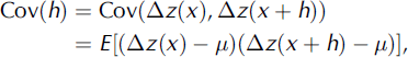
where μ is the mean of the elevation differences, or μ = E[Δz(x)]. Implicit in this description is the assumption of ‘first- and second-order stationarity’. In the current application, this means that the mean, μ, and the variance, , of the elevation difference are constant in space. For the practical application of the theory, this requires that there be no large-scale trends in the data and that there is no significant variation in the variance in space.

The auto-covariance is further related to the auto-variance, Var(h), by

(3)

In geostatistics the most frequently used auto-variance concept is the semi-variance or semivariogram, γ(h), when it is presented as a function of lag. This is simply half the auto-variance (Equation (3)), and is written as

(4)

where the covariance at h = 0, Cov(0), is equivalent in our application to the variance of the elevation difference, , such that

(5)

Equations (1), (4) and (5) can be combined to derive a relationship for the variance of the spatially averaged elevation difference, , in terms of the semivariogram and the variance of the elevation difference, :

(6)

The reason for expressing in terms of the semivariogram, γ(h), is that it is used extensively in geostatistical applications to specify the spatial variance, particularly for interpolation using kriging methods. The empirical semivariogram can be calculated from the available data and fitted with an analytical semivariogram model. There are a number of well-established models that can be used to describe the semivariogram (e.g. spherical, exponential and Gaussian models). For more details concerning the above definitions, and geostatistics in general, the reader is referred to texts such as Reference Webster and OliverWebster and Oliver (2001) and Reference CressieCressie (1993) from which Equations (1–6) have been adapted.

3.2. Estimating the spatially averaged uncertainty

Equation (6) states that in order to estimate the variance of the spatially averaged elevat{ = 0 }on difference, it is necessary to calculate the mean of the spatial covariance, the right-hand side of Equation (6). Spatially, this is achieved by integration over an area, A, and dividing by that area, i.e.

(7)

Converting the above integral to polar coordinates and assuming the area, A, is a circular region of radius L, such that A = πL ², Equations (6) and (7) can be combined to give

(8)

Since the semivariogram, defined in Equation (4), approaches when the covariance approaches 0, we also expect the integral in Equation (8) to approach 0 over sufficiently large distances.

3.3. Integration of an analytical form of the semivariogram

In order to solve Equation (8) we use an analytical function to describe the semivariogram. We choose the spherical equation (Reference Webster and OliverWebster and Oliver, 2001) that is commonly applied as a semivariogram model for kriging applications. In the following derivation, only a single isotropic spherical model is evaluated, for demonstration purposes. In the Appendix the result of the integration is also provided for a combined, or double-nested, model that uses two spherical models with different parameters. This model accommodates different scales of variance, as found in the data provided below.

A spherical semivariogram model is described by

(9)

where c = c ₀ + c ₁, c ₀ is known as the nugget, c ₁ the sill and a ₁ is the range; δh is the Kronecker delta part of the semivariogram that describes the correlation of a point with itself. A visual representation of these parameters, for the nested model, is provided in the Appendix (Fig. 13). Traditionally the nugget variance was introduced in mining applications to represent small-scale discontinuities introduced by solid ‘nuggets’ of minerals. In other spatial applications, such as here, it generally refers to unresolved scales of variance, i.e. variance on scales less than the sampling distance, and represents the spatially uncorrelated variance. The range indicates the distance within which some correlation exists between spatially separated points; at distances larger than the range there is no correlation. The sill, c ₁, is the maximum spatially correlated variance. The addition of this with the nugget, c ₀, represents the total variance, c, for distances greater than the range, i.e. c = c ₀ + c ₁, and should be equivalent to if Equation (4) is to be consistent over large distances, reflecting the assumption of stationarity, i.e.

(10)

Equation (8), after implementation of Equations (9) and (10),can be integrated to provide the following expression for the variance of the spatially averaged elevation difference, :

(11)

In Equation (11) we have replaced the Kronecker delta, δh, with the sampling distance, Δh. This parameter is defined in Equation (12) such that the sampling grid area, Δx ², is equivalent to the integrated area out to Δh. This allows the general application of the method to gridded data of spacing Δx:

(12)

For pure-nugget semivariograms, i.e. c ₁ = 0, Equation (11) is equivalent to the assumption of totally uncorrelated data and will provide the same relationship as the division of by the factor n, where n is the number of gridpoints over which the elevation difference is averaged.

In Figure 1 the influence of the nugget and range parameters on the spatially averaged uncertainty is visualized. Increasing the range clearly has a significant influence on the uncertainty estimates, with larger-scale spatial correlation leading to larger uncertainties for any given averaging area. An increasing nugget fraction of the total variance leads to decreasing uncertainties for any given averaging area, since the uncorrelated contribution to the total variance increases.

Fig. 1. Normalized standard deviation, σ_A /σ _Δz, of the spatially averaged elevation difference as a function of the averaging area (logarithmic scale), based on Equation (11). (a) The effect of a progressive doubling of the semivariogram range, a ₁, on the standard deviation, for the case where the nugget variance c ₀ = 0. (b) The effect of increasing the proportion of the nugget total variance, c ₀/c, where the range used for this example is 400 m.

For integration distances L > a ₁ (i.e. for distances over which there is no correlation) the integral decreases with the inverse of the area. Indeed, in many applications where the scale of the variance, represented by the range, a ₁, is smaller than the typical distance over which the integration is performed, Equation (11) can be interpreted in a simpler manner. Given a spherical semivariogram form with no nugget (i.e. c ₀ = 0 and c ₁ = c), an effective ‘correlated’ area, A _cor can be defined that is uncorrelated on scales larger than its size. This can be written as:

(13)

and the variance of the mean of the area, A, would then be approximated by:

(14)

Equation (14) represents the simplest outcome of the method. There may, however, be multi- or large-scale variance in the elevation difference data, such that the area to be averaged over is within the determined correlation range, especially if individual regions, such as the ablation area of a glacier, are to be assessed. Even so, Equation (14) provides a ‘rule of thumb’ when assessing the likely uncertainty in the spatial average of the elevation difference, when the area to be averaged over is larger than the determined correlation range.

4. Application Region and Dataset

4.1. Western Svartisen

The western Svartisen ice cap is located at ∼67° N, 14° E in a maritime climate in northern Norway and ranges in elevation from 10 to 1595 m a.s.l. (Fig. 2). The ice cap is the second largest glacier on mainland Norway, with an area of 190 km². NVE has performed traditional mass-balance measurements on the outlet glacier Engabreen annually since 1970. Reference Kjøllmoen, Andreassen, Engeset, Elvehøy and JacksonKjøllmoen and others (2003) report a positive cumulative mass balance of 22 m w.e. from 1970 to 2002 for the Engabreen drainage basin.

Fig. 2. Map of Svartisen, Norway. The grey area shows the extent of the ice cap and black curves outline the Engabreen and Storglombreen drainage basins.

4.2. Photogrammetrical elevation data

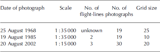
Vertical aerial photographs were collected for western Svartisen in 1968, 1985 and 2002 (Table 1). The 1968 DEM was digitized earlier by the Norwegian Mapping Authority from an analogue contour map. A triangular irregular network (TIN) was constructed from the analogue contour map and the DEM was interpolated from the TIN using bilinear interpolation.

Table 1. Photograph and DTM information

DEMs are constructed from digital photogrammetry for the years 1985 and 2002 using the software SocetSet and ImageStation. In the photogrammetrical software, block adjustment was conducted after registering the GCPs and tie points in the stereo models. The digital images in the stereo models were matched to identify identical features, and elevations were calculated according to the determined recording geometry. Mismatched points were edited manually. Where elevation points could not be measured, mainly in the low-contrast snow regions, interpolation was conducted using the photogrammetrical software package, to form a regular grid of elevation data (a DEM). The geodetic mass balance was calculated from these DEMs after conversion of volume changes to water equivalents.

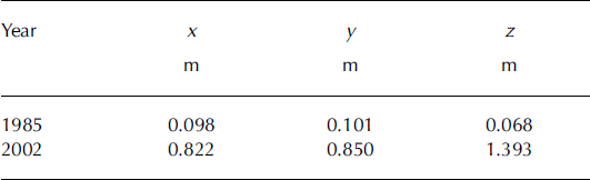
The root-mean-square (rms) error for the GCPs in the absolute orientation is shown in Table 2. Elevation contours over the three years are shown in Figure 3, before any detrending was carried out. The successful matching points from the digital photogrammetry of the 2002 photographs are shown in Figure 4. As the figure illustrates, there are relatively few measured elevation points in the snow-covered area in the centre. There are more points in the 1985 DEM in the snow area, and only the results for the 2002 DEM are included to show the worst case.

Fig. 3. Elevation contours for the three years. The contour interval is 20 m. The drainage basins are indicated: 1. Memorgebreen; 2. Fonndalsbreen; 3. Engabreen; 4. Dimdal–Frukosttindbreen; 5. Northern-part; 6. Storglombreen; 7. Flatisvatnet; 8. Nordfjord-breen. The grey area shows the coverage of the laser measurements.

Fig. 4. Measured points (black) in the DEM from 2002. The glacier area is shown in grey.

Table 2. The rms errors of the GCPs used for constructing DEMs in a digital photogrammetrical workstation

5. Application and Results: Geodetic Mass Balance and Estimated Uncertainties

5.1. Detrending of photogrammetrical-elevation difference data

The photogrammetrical DEMs are subtracted for both periods (1968–85 and 1985–2002). A detrending function, using least-squares fitting to the data, is determined over bedrock areas, and the function is applied to both bedrock areas and glaciated areas.

Some areas are excluded when determining the detrending function. Western Svartisen is situated in a steep mountainous area, but only 2% of the ice cap has a slope >30°. Areas steeper than 30°, and shadow areas where few identical features are matched in the stereo pairs, are excluded when determining the function. Exclusion of steep mountainsides reduces elevation differences that stem from horizontal shifts of the DEMs due to uncertainty in the absolute orientation.

Zeroth-, first-, second- and third-order detrending functions are evaluated. The zeroth order represents a constant value. A second-order detrending function is eventually used because third-order terms did not reduce the rms errors of the detrending function substantially. The rms errors of the detrending functions for the four different orders and the differences between orders are shown in Table 3.

Table 3. Rms errors for different orders of the detrending functions for the two periods. The differences between the lower-order functions are shown in parentheses. The different orders are: zeroth – constant in space; first – linear; second – quadratic; and third – cubic

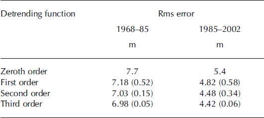
The mean difference between the 1985 DEM and the 1968 DEM over bedrock before the detrending function is applied is −0.14 m, which means that the 1985 DEM is, on average, slightly lower than the 1968 DEM. The difference between the 2002 DEM and the 1985 DEM over bedrock before the detrending is applied is 0.75 m. The range of the data points in the second-order detrending is −3.3 to 4.2 for 1968–85, and −6.1 to 4.6 for 1985–2002.

5.2. Semivariograms for bedrock

We estimate the elevation errors for both periods by investigating the semivariograms of the detrended elevation differences over bedrock. Semivariograms are used in order to determine the scale at which the elevation differences correlate (range) and to determine the nugget and sill parameters. The empirical semivariograms are derived by binning the variances at different discrete lag distances. In order to capture the different scales, binning is carried out at 25 m intervals for scales <1 km, and at 200 m intervals for scales <20 km. Individual spherical semivariogram models are fitted to the two scales to identify the different scales and their semivariogram parameters. Fitting is carried out using an unconstrained non-linear optimization technique for all three parameters. To combine the individually determined semivariograms into a double semivariogram the fitted short-scale sill + nugget variance is subtracted from the fitted long-scale sill + nugget variance to determine the long-scale sill, c ₂. The nugget variance, c ₀, and short-scale sill variance, c ₁, are then determined by subtracting the long-scale semivariogram from the short-scale empirical semivariogram and refitting.

Two scales of variance are identified for the 1968–85 elevation-difference data, with ranges of 430 and 3100 m. The fitted semivariograms are shown in Figure 5 and the fitted parameters are listed in Table 4. The larger scale is less well pronounced and only adds a small amount of variance to the smaller scale.

Fig. 5. Semivariograms for the 1968–85 bedrock elevation difference: (a) the empirical values are binned using 25 m bins over a distance of 1 km; (b) 200 m bins are used over a distance of 20 km. A single spherical semivariogram model is fitted to the data and shown as a solid curve. Although there is significant scatter on the larger scale (b) the fitted semivariogram indicates a weak larger-scale variance with a range of 3100 m. See Table 4 for the fitted semivariogram parameters.

Table 4. Table showing the deduced semivariogram parameters of nugget (c ₀), sill ₍ c ₁, c ₂) and range (a ₁, a ₂) for the double-spherical model described in the Appendix

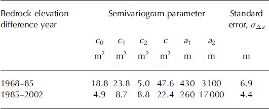
Two distinct scales of variance are identified for the 1985–2002 elevation difference, at 260 and 17 000 m, and are shown in Figure 6. The smaller-scale variance is similar to that seen in the 1968–85 bedrock semivariograms (Fig. 5) and the fitted parameters are listed in Table 4. The large-scale variability seems to indicate a trend that has not been totally removed by the detrending. Though the larger scale may be interpreted as a spatial trend in the data, its existence will contribute significantly to the uncertainty when averaging is carried out.

Fig. 6. Semivariograms for the 1985–2002 bedrock elevation difference: (a) the empirical values are binned using 25 m bins over a distance of 1 km; (b) 200 m bins are used over a distance of 20 km. A single spherical semivariogram model is fitted to the data and shown as a solid curve. There is a discernible larger-scale variance (b) that can be seen to vary with lag distance. See Table 4 for the fitted semivariogram parameters.

5.3. Uncertainty in the spatially averaged elevation difference

Based on the values of sill, nugget and range that are determined by fitting of the semivariograms (Table 4) the uncertainty, σ_A , in the spatial average elevation difference is calculated as a function of the averaging area using Equation (A2). The results are shown in Figure 7. In spite of the higher standard error ₍ σ _Az) for the 1968–85 differences, the uncertainty decreases faster due to the relatively short spatial scale of the variance. The standard error for the 1985–2002 differences is lower, but due to the longer spatial scale of the variance, the uncertainty decreases more slowly. Also indicated in Figure 7 are the estimated uncertainties assuming the standard errors, σ _Az, to be totally correlated and totally uncorrelated in space.

Fig. 7. Uncertainty, σ _A, of the spatially averaged elevation difference as a function of the averaging area (logarithmic scale) based on the analysis of the elevation difference statistics determined over bedrock (Table 4): (a) the 1968–85 result and (b) the 1985–2002 result. Included in the plots, for reference, are the estimated uncertainties assuming that the standard error of the elevation difference is totally uncorrelated (thin red continuous curve) and totally correlated (thin red dotted line) in space.

5.4. Geodetic mass balance and its uncertainty

The geodetic mass balances of the western Svartisen ice cap and the eight different drainage basins are listed in Table 5. The calculated surface-elevation change is shown in Figure 8. In both periods all the drainage basins have negative or close to zero mass balance, with Memorgebreen as most negative in the first period. In the period 1985–2002 the Northern-part drainage basin is most negative, while Memorgebreen is not mapped. The mass balances of the two largest drainage basins, Engabreen and Storglombreen, are less negative than the mass balances of the other glaciers.

Fig. 8. Surface-elevation change for the western Svartisen ice cap: (a) 1968–85; (b) 1985–2002. The black curves mark the different drainage basins. The hatched area is where poor contrast is found.

Table 5. Summary of the mass-balance calculations and uncertainty estimates for western Svartisen and its drainage basins for the two investigation periods. Provided are the drainage basin area, the geodetic mass balance, the contribution of the spatial average uncertainty to the mass balance and the total mass-balance uncertainty. Drainage basins without complete coverage are not included

In addition to the uncertainty in the elevation difference, the total uncertainty in the geodetic mass balance depends on the ablation corrections and density assumptions. The ablation correction is calculated based on the sum of positive degree-days and the glacier melt rate calculated by Reference SchulerSchuler and others (2005). Because the sum of positive degree-days is measured only at the glacier plateau and the glacier melt rate is calculated only for Engabreen, uncertainties are introduced. These uncertainties are the same for all drainage basins. The density of the glacier mass is assumed to be constant over the 34 year period, and this also introduces uncertainties. Here the uncertainties vary from drainage basin to drainage basin depending on the size of snow, firn and blue-ice areas in the basins. Further information on the calculation of ablation and density uncertainties can be found in Reference Haug, Rolstad, Elvehøy, Jackson and Maalen-JohansenHaug and others (2009). Ablation corrections and density uncertainties are assumed to be uncorrelated with the elevation measurements, and the total uncertainty in geodetic mass balance is estimated using standard error propagation for uncorrelated variables. In Table 5 the estimated uncertainties, in terms of standard deviation, are shown for each of the drainage basins. These are based on the geostatistical analysis of the bedrock variance as shown in Figure 7, as well as on the ablation and density corrections. For the first period, both sources of uncertainty contribute to the mass-balance uncertainty. For the second period the elevation difference uncertainties are significantly larger than the other uncertainties and the latter hardly contribute to the total uncertainty.

6. Application and Results: Comparison of Laser Scanning and Photogrammetricalelevation Data

The DEM derived from laser scanning is subtracted from the 2002 photogrammetric DEM, and the result is shown in Figure 9. These two DEMs were separated by a period of 3 days. Large elevation differences are found in the snow-covered areas, where elevation differences are as high as ±15 m. This area corresponds to the area with few successful matching points due to poor contrast in the 2002 digital photogrammetrical DEM, shown in Figure 4. In this area most elevations are based on bilinear interpolation of the available matching points (Fig. 9). When the elevation difference over bedrock is calculated, areas containing forest are avoided, since the DEM constructed from photogrammetry reflects the vegetation height instead of the bedrock height. No spatial detrending is carried out on the elevation difference. The mean difference between the two DEMs, zeroth-order detrending, is subtracted from the elevation difference map.

Fig. 9. The difference between the 2002 DEM constructed from photogrammetry and the DEM constructed from laser scanning. Green indicates areas where the DEM constructed by photogrammetry has higher elevations, and red indicates areas where it has lower elevations. The black curve marks the area of poor contrast in the 2002 DEM.

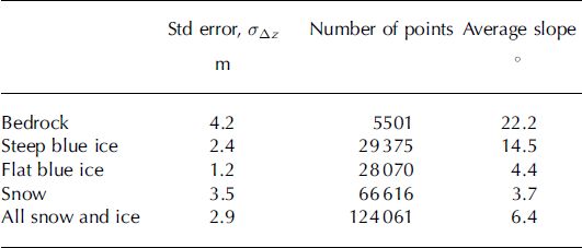
We want to investigate whether the geostatistics of elevation errors determined over bedrock are representative for glacier surface types, and three different glacier surface types are identified according to surface properties and slope. The elevation gradients of the laser DEM are calculated from the eight neighbouring gridcells with 20 m resolution. To define continuous-surface-type areas, the areas are separated manually into four surface types and the average gradient values are calculated for the areas. The surface-type areas of bedrock, flat blue ice, steep blue ice and snow are shown in Figure 10, and their corresponding average slopes and standard errors are given in Table 6.

Fig. 10. (a) The areas of the different surface types; and (b) the elevation gradients for the same areas.

Table 6. Standard error of the difference between the 2002 DEM constructed from photogrammetry and the DEM constructed from laser scanning for the different surface types. Also shown are the average slopes of the different regions

Semivariograms of the elevation difference grid (Fig. 9) have been made for the same four surface types (Fig. 10). From these the spherical semivariogram parameters, as described above, have been deduced and are given in Table 7. The empirical semivariogram and the fitted spherical semivariograms are presented in Figure 11. For these surfaces, only one scale of variance was found.

Fig. 11. Semivariograms of the difference between the 2002 DEM constructed from photogrammetry and the DEM constructed from laser scanning for four different surface types: (a) all snow and ice; (b) snow (interpolated); (c) bedrock; (d) steep blue ice. Empirical values of the variance are determined by binning in 25 m bins. A single spherical semivariogram model is fitted to the data and is shown as a solid curve. See Table 7 for the fitted semivariogram parameters.

Table 7. The deduced semivariogram parameters of range (a ₁), nugget (c ₀), sill (c ₁) and the square root of sill plus nugget (c ^1/2), for the different surface types. The last parameter reflects the standard errors (σ _Az ) in Table 6

The differing spatial ranges of the correlation of the surfaces types, as well as their standard errors, have consequences for the estimated uncertainty when spatially averaging to obtain average elevation differences. Using Equation (11) and the semivariogram parameters presented in Table 7, it is possible to estimate the uncertainty for each of the surface types described above as a function of averaging area. This is presented in Figure 12. The uncertainty in snow is the largest of all the surface types, due to the combination of a high standard error, σ_Δz, and a long correlation distance (range). Even though bedrock has the highest standard error (Table 6), it has a short correlation distance (range) and also an estimated nugget variance that is approximately half the total variance. As a result, the spatially averaged uncertainty is low compared to snow. The two blue-ice types have very similar uncertainties, close to that calculated for bedrock.

Fig. 12. The estimated uncertainty in the spatially averaged elevation difference between the laser and photogrammetric DEMs presented as a function of averaging area (logarithmic scale). These are based on the semivariogram parameters listed in Table 7 and the application of Equation (11).

7. Discussion

Comparison of the traditional and geodetic mass balance for Engabreen drainage basin shows that the two methods give significantly different results. For the period 1970–2002 the cumulative traditional mass balance is 22 m w.e. (Reference Kjøllmoen, Andreassen, Engeset, Elvehøy and JacksonKjøllmoen and others, 2003). The geodetic mass balance for the period 1968–85 is −2.1 ± 1.2 m w.e., and from 1985 to 2002 it is −0.3 ± 2.6 m w.e. Given the validity of the uncertainty assessment carried out here, the deviation cannot be explained by the uncertainty in the geodetic mass balance. Reference Elvehøy, Jackson and AndreassenElvehøy and others (2009) showed that incorrectly defined drainage basin boundaries can lead to significant differences in mass-balance estimates for Engabreen, but these are not sufficient to explain the differences between the geodetic and traditional mass-balance methods. Possible additional explanations for the excess of mass according to the field measurements are annual systematic errors. It is known that stakes sink into the snowpack and that snow probes deviate from the vertical, especially in high-accumulation areas. There may also be basal melting and internal ablation that is not accounted for in the traditional mass budget. These explanations require further investigation.

The elevation differences of the photogrammetrical DEMs are analysed to determine the spatial correlation, and three spatial scales are found: (1) at hundreds of metres (260 and 430 m for both periods); (2) at kilometres (3100 m for the first period); and (3) at tens of kilometres (17 000 m for the second period). We suggest that the hundred-metre scales are due to the matching procedure in the digital photogrammetrical software for identification of conjugate points in the stereo models for elevation measurements. Pyramids of coarse-resolution images are established and the matching is typically conducted on squares of 15 × 15 pixels, which may correspond to ground coverage of some hundreds of metres. We suggest that the weak intermediate kilometre scale may be due to block instability from the aerotriangulation; the individual stereo models are not correctly orientated relatively. The scale of the aerial photographs from 1968 and 1985 is 1 :35 000,which yields a stereo ground coverage of a few kilometres for each stereo model, similar to the 3100 m scale of spatial correlation that is found for this period. The third scale of correlation, of tens of kilometres, is expected to be due to the absolute orientation of the stereo models in the block. We emphasize that our interpretations are tentative in nature and that further photogrammetrical experiments must be conducted to verify these.

The intermediate kilometre variance scale is not well pronounced and is only evident in the 1968–85 elevation difference data. The evaluation of the required polynomial order of the detrending function for the elevation differences shows that third-order terms have little influence on the rms error, indicating that the blocks are stable. According to this result, the stereo models should be well oriented relatively, which may explain the low pronunciation of the intermediate kilometre scale. It is our impression that the 2002 block is stable, since tie points are extensively used during the aero-triangulation, and for the period 1985–2002 there is no kilometre correlation scale.

The largest, several kilometre, correlation scale is found only for the last period; we assume that this is due to poor geo-referencing of parts of the 2002 DEM. The geo-referencing is less accurate for this DEM mainly because visible GCP targets were not deployed in the terrain at all corners of the model, so some areas have many, well-defined GCPs and some areas have fewer or poorly defined GCPs.

The spatially averaged variance of the semivariogram (Equation (11)) shows that the scale of the correlation, indicated by the semivariogram parameter of range, is important in determining the rate of reduction in the uncertainty with increased averaging area. The uncertainty of the spatial average of the elevation differences decreases quickly as a function of averaging area during 1968–85, but more slowly for 1985–2002, as seen in Figure 7. This is due to the considerably shorter correlation scale for the first period (Table 4). The large correlation scale for the second period is, as suggested, most likely caused by less accurate geo-referencing, and this emphasizes how important it is for accuracy that visible GCP targets are deployed in the terrain and properly identified in the images.

The scales of correlation found for the various surface types, using the comparison of laser and photogrammetrical DEMs, may be due to uncertainties in both DEMs. These errors may vary for the two methods depending on surface types and slopes. There may, for instance, exist a correlation scale similar to the width of the laser scan (∼600 m). However, in this paper we do not focus on uncertainty contributions from laser measurements and we assume, based on the comparison of laser data with GPS measurements, that the laser measurements are the more accurate of the two. Standard errors of 0.08 m were found, when compared with GPS measurements, for the laser altimetry data (Reference Geist, Elvehøy, Jackson and StötterGeist and others, 2005).

Different standard errors are found for the elevation difference between the photogrammetrical and laser data for the four surface types (Table 6). The estimated value is largest for bedrock, which can be attributed to both its rougher surface and its steeper slope. When the slope and roughness increase, small orientation errors lead to larger elevation differences, and increased geometric distortion leads to less accurate matching results for the photogrammetrical elevation measurements. On blue ice, higher standard deviations of the elevation differences occur over steeper than over flat areas, as a result of both the larger slope and the advection of crevasses over the 3 day interim period. The velocities in the crevassed steep blue-ice part of the glacier are up to 0.8 m d⁻¹ at the time of the year when measurements were made (Reference Jackson, Brown and ElvehøyJackson and others, 2005), which will lead to a small shift in the crevasse pattern. Laser beams may also penetrate deeper into the crevasses to give different elevations from photogrammetrical-elevation measurements. For the case of snow, the high standard deviation of the elevation differences is due to the limited availability of data in this region. The resulting variability, and correlation scale, in this area depends on the spatial distribution of the available data, as well as on the interpolation method used to provide complete coverage for the photogrammetrical DEM.

Correlation scales for the laser and photogrammetricalelevation differences are determined for the four surface types (Table 7), and the results reflect the nature of the different surfaces. Bedrock, for instance, has a very short correlation range, with the fitted semivariogram model range found to be just 140 m. Snow and flat ice surfaces indicate a larger range of 740–790 m, with much smaller nugget contributions. This is the expected result, that flatter and more homogeneous regions are correlated over longer distances. However, the bedrock and blue-ice semivariograms also contain a large nugget component relative to the sill (Table 7), indicating that a significant amount of the variance detected in these surfaces is not spatially correlated. This is in contrast to the snow surface, which has a very small nugget component relative to the sill, indicating stronger spatial correlation. This last point is the clear result of the spatial interpolation carried out in the snow-covered areas, leading to strongly correlated local trends on spatial scales less than the average distance between successful photogrammetric matching points.

The comparison of photogrammetrical-elevation data with laser scanning data for the various surface types shows that the scale of the spatial correlation depends strongly on the elevation gradient (Table 6). As glaciers are often flatter and smoother than the surrounding bedrock, this has implications for the estimation of uncertainties for the glacier based on statistics of elevation errors based on bedrock. The uncertainty will thus, in general, not reduce as quickly, with increasing averaging area, for a flat glacier surface as it would for steeper and rougher bedrock. Similarly, the standard errors of the flat ice areas should be lower than those for rock.

The geostatistical analysis of the different surface types indicates that the small-scale statistical characteristics of the different surfaces do vary to some degree, particularly for the case of snow where the spatial photogrammetrical sampling is poor. However, it is difficult to extrapolate these differences, found from the comparison of laser and photogrammetric DEMs, to the differences between two photogrammetric DEMs. Firstly, the bedrock elevation-difference semivariogram range is almost twice as large for the 1985–2002 photogrammetric DEM difference as it is for the 2002 laser/photogrammetric DEM difference and, secondly, the contribution of the nugget variance to the 2002 laser/photogrammetric DEM is much larger than that found for the 1986–2002 photogrammetric DEM difference. As such it is difficult to compare the two datasets directly. Despite this, there is a need to provide an alternative to just using bedrock statistics for application to snow-covered surfaces where photogrammetrical sampling is often poor. We recommend that the small-scale spatial characteristics of the bedrock difference be replaced over snow surfaces such that the nugget variance, c ₀, be set to 0 and the small-scale range, a ₁, be increased to 740 m. The total sill variance, c, should be kept the same.

To test the effect of this on the datasets available, the drainage basin mass-balance uncertainties (Table 5) are recalculated assuming the entire surface to be snow-covered, i.e. the worst case, using the snow-nugget and range parameters given above. The effect of this change is negligible for the 1985–2002 dataset, because the uncertainty is dominated by the large-scale correlations, which are assumed to be independent of surface type. For the 1968–85 dataset the effect over large scales is also minimal, an increase in σ_A of <0.1 m for both Engabreen and western Svartisen. There is a noticeable increase in the uncertainty for the smaller drainage basin Fonndalsbreen, where σ_A increases from 1.6 to 2.0 m as the result of the change in semivariogram parameters.

8. Conclusions

We have described and demonstrated a geostatistical method to estimate the uncertainty in the geodetic mass balance when using two DEMs that are spatially correlated. We found that there is a significant degree of spatial correlation in the elevation differences between two DEMs and that the uncertainty in the spatially averaged elevation change is dependent on both the scale of the spatial correlation and the standard deviation of the individual point errors. We applied the method to the western Svartisen ice cap and presented results for its geodetic mass balance and uncertainties, estimated from photogrammetric DEMs from 1968, 1985 and 2002. Further, we investigated the different geostatistical characteristics of bedrock and a range of glacier surfaces, using concurrent photogrammetric and laser altimetry measurements, to ascertain whether bedrock geostatistics were representative of glacier surface geostatistics.

We calculated the geodetic mass balance of western Svartisen using photogrammetry for the periods 1968–1985 and 1985–2002, and found it to be −2.6 ± 0.9 and −2.0 ± 2.2 m w.e., respectively. In the period 1985–2002 the two largest drainage basins, Engabreen and Storglombreen, showed a less negative mass balance than the other basins. The bulk of the accumulation area was situated within these two basins. For Engabreen drainage basin the geodetic mass balance was −2.1 ± 1.2 m w.e. for the first period, and −0.3 ± 2.5 m w.e. for the second period. This deviates considerably from the cumulative traditional mass balance, which was 22 m w.e. from 1970 to 2002.

The geostatistical nature of the elevation differences of the surrounding bedrock of western Svartisen has been assessed and their associated uncertainties have been estimated. The uncertainty in the elevation difference contributes significantly to the total uncertainty in geodetic mass balance, and we found large differences in the uncertainties for the two periods. The contribution of the elevation difference to the geodetic mass-balance uncertainty for 1968–85 is ± 0.4 m w.e., and for 1985–2002 it is ±2.1 m w.e. We suggest that the errors are largely due to inaccurate GCPs in some of the corners of the 2002 DEM.

Three correlation scales were found for the photogram-metrical data at a few hundred metres, at a few kilometres and at tens of kilometres. The short scale is hypothesized to be due to the automatic digital photogrammetrical-matching procedure for elevation measurement in various terrain types, the intermediate scale may be due to poor relative orientation of the stereo models in the block, while the largest scale is likely to be the result of absolute orientation errors. The intermediate scale is found, in these datasets, to be very weak.

Photogrammetrical data were compared to laser scanning data to evaluate how representative the statistics of elevation errors determined over bedrock are for the glacier surface statistics, and thus the estimated uncertainty. We found that the scale of the correlation, represented by the semivariogram parameter of range, depends on the elevation gradient and that the form of the semivariogram may differ between surfaces. The largest difference between bedrock and other surface types occurs over snow, where there are few photogrammetrical matching points due to poor contrast. This leads to a stronger small-scale spatial correlation, which is a result of the poor sampling density and the application of interpolation. To mitigate this, we recommend applying an alternative range and nugget value to snow-covered areas. However, tests on the current datasets show that these alternative parameters, applied to the small correlation scale, have a very limited effect on the overall uncertainty, since this is dominated by the larger-scale correlation when averaging over extended areas.