


1. Introduction
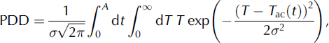
The positive degree-day model is a parameterization of surface melt widely used for its simplicity (Reference HockHock, 2003). Melt is assumed to be proportional to the number of positive degree-days (PDD), defined as the integral of positive Celsius temperature Tover a time interval A:

When modelling glaciers on the multi-millennium timescale needed for spin-up simulations or palaeo-ice-sheet reconstructions (e.g. Reference Charbit, Dumas, Kageyama, Roche and RitzCharbit and others, 2013), daily or hourly temperature data are usually not available and PDDs are typically calculated over 1 year using an average annual temperature cycle. Sub-annual temperature variability around the freezing point, however, significantly affects surface melt on a multi-year scale (Reference Arnold and MacKayArnold and MacKay, 1964). It is commonly included in models by assuming a normal probability distribution of T of known standard deviation u around the annual cycle T ac (Reference BraithwaiteBraithwaite, 1984). PDDs can then be computed using a double-integral formulation of Reference ReehReeh (1991),
or more efficiently using an error function formulation of Reference Calov and GreveCalov and Greve (2005),

These approaches have been implemented and used in several glacier models (e.g. Reference Letréguilly, Reeh and HuybrechtsLetréguilly and others, 1991; Reference GreveGreve, 1997; Reference Huybrechts and de WoldeHuybrechts and de Wolde, 1999; Reference Seddik, Greve, Zwinger, Gillet-Chaulet and GagliardiniSeddik and others, 2012; Reference Charbit, Dumas, Kageyama, Roche and RitzCharbit and others, 2013). However, with the exception of an available parameterization for the Greenland ice sheet (Reference Fausto, Ahlstrøm, Van As and SteffenFausto and others, 2011), σ is often assumed constant in time and space, despite its large influence on modelled surface melt and subsequent ice-sheet geometries (Reference Charbit, Dumas, Kageyama, Roche and RitzCharbit and others, 2013). Here I showthat σ is in fact highly variable spatially and seasonally, which has significant effects on PDD and surface mass-balance (SMB) computation.
2. Temperature Variability
Using the European Centre for Medium-Range Weather Forecasts’ ERA-Interim reanalysis data (Reference DeeDee and others, 2011) for the period 1979–2012, a monthly climatology is prepared, consisting of long-term monthly mean surface air temperature, long-term mean monthly precipitation and long-term monthly standard deviation of daily mean surface air temperature. Standard deviation is calculated using temperature deviations relative to the long-term monthly mean for the entire period, in order to capture both day-to-day and year-to-year variations of surface air temperature. Daily mean surface air temperature is computed beforehand as an average of the four daily analysis time-steps (00:00, 06:00, 12:00, 18:00), to avoid variability associated with the diurnal cycle. Since the annual temperature cycle is not removed from the time series, this approach may lead to slightly overestimated standard deviation values in spring and autumn when temperature varies significantly between the beginning and the end of a month.
Computed standard deviations range from 0.32 to 12.63 K, with a global annual average of 2.02 K. There is a tendency for higher values over continental regions (Fig. 1). Additionally, computed standard deviation follows an annual cycle, with a winter high and a summer low. This extends the conclusions obtained by Reference Fausto, Ahlstrøm, Van As and SteffenFausto and others (2011) over Greenland to non-glaciated regions, where summer temperatures are not constrained by 0°C by an ice surface.

Fig. 1. Spatial distributions of standard deviation of daily mean surface air temperature for January (top) and July (bottom) based on the ERA-Interim reanalysis data for the period 1979–2012. The maps show higher values in winter and over continental regions (Reference DeeDee and others, 2011).
3. Positive Degree-Days
A reference PDD distribution, hereafter PDDERA, is computed using Eqn (3) over 1 year and the monthly climatology described above. Furthermore, annual PDDs are computed using four additional, simplifying scenarios:
-
1. using Eqn (1) (PDD0);
-
2. using Eqn (3) with σ = 5 K, a value commonly used in ice-sheet modelling (Reference Huybrechts and de WoldeHuybrechts and de Wolde,1999; Reference Seddik, Greve, Zwinger, Gillet-Chaulet and GagliardiniSeddik and others, 2012; Reference Charbit, Dumas, Kageyama, Roche and RitzCharbit and others, 2013) (PDD5);
-
3. using an annual mean of standard deviation (PDDANN);
-
4. using a boreal summer (June–August (JJA)) mean of standard deviation (PDDJJA).
All four scenarios lead to significant errors in PDD estimates when applied on a continental scale (Fig. 2). Assuming zero temperature variability (PDD0) generally underestimates PDD values. Assuming σ = 5 K (PDD5) reduces errors in continental North America and Eurasia but overestimates PDD values in coastal locations and over the Greenland ice sheet. Using annual mean (PDDANN) or summer mean (PDDJJA) standard deviation generally yields smaller, yet significant, errors.

Fig. 2. PDD error (ΔPDD i = PDD i − PDDERA) over the Arctic using (a) zero temperature variability, (b) fixed temperature variability (σ = 5 K), (c) mean annual temperature variability and (d) mean summer temperature variability.
4. Surface Mass Balance
For each scenario, SMB is computed using a simple annual PDD model (github.com/jsegu/pypdd). Accumulation is assumed equal to precipitation when temperature is below 0°C, and decreasing linearly with temperature between 0 and 2°C. Melt is computed using degree-day factors of 3 mm °C−1 d−1 for snow and 8 mm °C−1 d−1 for ice (Reference Huybrechts and de WoldeHuybrechts and de Wolde,1999). Surface mass balance is computed over weeklong intervals prior to annual integration using a scheme similar to that implemented in the ice-sheet model PISM (Parallel Ice Sheet Model; www.pism-docs.org).
Over Greenland, using summer mean standard deviation in the SMB calculation (SMBJJA) gives smaller errors than other simplifying scenarios (Fig. 3). This confirms recent results obtained by Reference Rau and RogozhinaRau and Rogozhina (2013) from the ERA-40 reanalysis data. However, in all four cases, large SMB errors occur along the margin where most of the melt processes take place.

Fig. 3. Surface mass-balance error (ΔSMBi = SMBi – SMBERA) over Greenland using the same scenarios as in Figure 2.
5. Conclusion
Using gridded climate products, temperature variability can be assessed quantitatively on the continental scale. Monthly standard deviation of daily mean surface air temperature is highly variable both spatially and seasonally. When using standard deviation PDD formulations (Reference BraithwaiteBraithwaite, 1984; Reference ReehReeh, 1991; Reference Calov and GreveCalov and Greve, 2005), approximations of constant standard deviation do not hold on the continental scale and introduce significant errors in modelled PDD and SMB, which have immediate implications for numerical modelling studies of present-day and former glaciations. Under the assumption of a normal distribution of temperature around the annual cycle, numerical glacier models that use an annual PDD scheme should therefore implement spatially and seasonally variable standard deviations of daily mean surface air temperature in order to more realistically capture patterns of surface melt.
Standard-deviation and mass-balance data presented in Figs 1–3 were prepared globally and are available online at http://www.igsoc.org/hyperlink/13j081/.
Acknowledgements
I thank Caroline Clason, Ping Fu, Christian Helanow, Andrew Mercer, Arjen Stroeven and Qiong Zhang for help in preparing the first version of this correspondence, Irina Rogozhina for multiple advice on text and figures, Constantine Khroulev for sharing details of PISM’s PDD implementation through e-mail, and Regine Hock and Roger Braithwaite for constructive reviews and suggestions for improvements. Partial funding was provided by the Swedish Research Council (VR) to Stroeven (No. 2008- 3449) and Stockholm University.
7 September 2013


