Introduction
Ice cores recovered near the flow divide of four high-altitude ice caps (Fig. 1) in equatorial and mid-latitude regions are valuable sources of climatic records (Reference Thompson, Mosley-Thompson, Dansgaard and GrootesThompson and others, 1986, Reference Thompson1989, Reference Thompson1995a, Reference Thompson1997). The ice has thinned and stretched with time due to the force of the Earth–s gravity acting on the glacier. Measurements of surface velocity are needed to construct accurate numerical models of ice flow, which aid in dating the ice with depth (Reference Thompson, Bolzan, Brecher, Kruss, Mosley-Thompson and JezekThompson and others, 1982). The surface velocity is measured by observing the change in position between two surface stakes over time using geodetic techniques. The observed velocity is non-uniform and ranges from 1 to 20 m a-1, within a few hundred meters of the flow divide.
On high-altitude ice caps the position of a surface stake network measured during periodic visits within the 1–3 years of an active field program with conventional geodetic observations (electronic distance measurement (EDM), and horizontal and vertical directions) and/or space geodetic observations (the global positioning system (GPS)) is an effective approach to measure the surface velocity, because it is desirable the uncertainty in the surface velocity measurement be within a few per cent of the velocity magnitude (i.e. ? – 10 cm a-1). Remote-sensing techniques that register sequential visible and near-infrared imagery taken from satellite, aerial and terrestrial platforms all rely on tracking the motion of an identifiable surface feature, typically lacking in the accumulation zone enclosing the flow divide, and have uncertainties of 1–20 m a-1 (Reference Bindschadler and ScambosBindschadler and others, 1991; Reference Brecher and ThompsonBrecher and Thompson, 1993; Reference Fastook, Brecher and HughesFastook and others, 1995). Satellite radar interferometry (ISAR) can sense the mm-range change along the line of sight from the satellite to the footprint of the radar signal on the glacier surface between two successive passes of the satellite that occur within a span of a few days. After a few days the images decorrelate because the surface features change, so annual velocity must be extrapolated from the rate determined over a few days, increasing the uncertainty to 0.6–1.0 m a-1 (Reference Goldstein, Engelhardt, Kamb and FrolichGoldstein and others, 1993; Reference Rignot, Forster and IsacksRignot and others, 1996). While the field measurements between stakes are labor-intensive, they are a cost-effective approach providing adequate spatial coverage and precision to measure surface velocity on remote small ice caps.
To capture the spatial variation in non-uniform surface flow near the flow divide on typical ice caps, a network of connected chains of stakes is used. Reference NyeNye (1959) implemented repeated direct measurements of the distance and horizontal angle of five stake networks to determine the principal strains. Reference MacAyealMacAyeal (1985) introduced an additional refinement showing that in parallel and nearly uniform flow fields the precision of the principal strain estimates can be improved by using multiple-center-stake rosettes. In a non-uniform flow field a typical network should consist of a grid of stakes separated horizontally by one ice thickness, and with a lateral extent at least five ice thicknesses downstream of the divide, and at least two ice thicknesses perpendicular to the downstream direction (Whillans and Reference Tseng, Whillans and van der VeenVan der Veen, 1989; Reference Van der Veen and WhillansVan der Veen and Whillans, 1992). If desired, the principal strains at locations within the network can be computed from the velocity gradients of the surrounding stakes (Reference BrunnerBrunner, 1979; Reference PatersonPaterson, 1994).

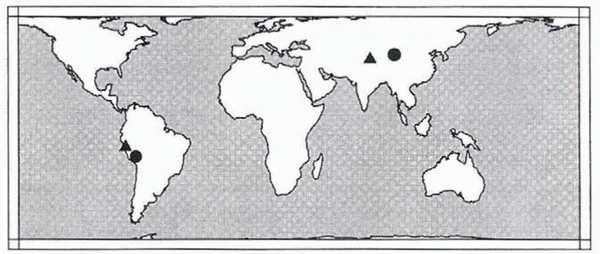
Fig. 1. Global map showing location of four surface strain networks established as part of the recovery of cores from high-altitude ice caps. Solid triangles show location of the Huascar–n and Guliya strain networks examined in this paper. Solid circles show location of Quelccaya and Dunde surface strain networks.
With the stakes placed to enclose the general flow pattern, designing a geodetic observation plan for the stake network begins with predicting, to first order, the anticipated magnitude and direction of the surface motion and the uncertainty in the surveyed stake positions. A mathematical model of glacial flow is used to predict the approximate motion (e.g. Reference Thompson, Bolzan, Brecher, Kruss, Mosley-Thompson and JezekThompson and others, 1982). The a priori geodetic observation precision estimates are typically available for the common geodetic observation techniques developed for purposes other than glaciology. However, the extreme cold and high-latitude/altitude environments may introduce systematic errors that are less significant in more benign environments (Reference Tseng, Whillans and van der VeenTseng and others, 1989). The primary design criterion is the position uncertainty that must be achieved for surveys separated by 1 or 2 years to determine the actual surface motion with a level of confidence. Specifically, the uncertainty in the measured velocity should be within a few per cent of the velocity magnitude. This criterion relies on the assumption that all geodetic observations are collected with their assumed random errors. If the geodetic observations contain blunders or systematic errors, then the velocity estimates are not of this quality.
Several steps are taken to minimize systematic errors and to guard against introducing blunders while simultaneously increasing the precision of the stake coordinate estimates. Systematic errors in distance observations are controlled by comparing EDM observations at a calibration range before and after field measurements (Reference FronczekFronczek, 1977) and by measuring the ambient air temperature and pressure to compute the refractive index. Systematic errors in direction observations are controlled by adjusting the vertical index of the theodolite and taking the mean of angles measured in both direct and reversed telescope orientations. Systematic errors in GPS observations are controlled by forming a linear combination of the two signals broadcast by the GPS satellites that is free of the first-order effects of the ionosphere, and by using a priori post-fit satellite orbits, modeling receiver clock drifts, and tropospheric refraction during data reduction (e.g. Reference LeickLeick, 1995).
Blunders are controlled by repeated observations and localized geometric checks. Repeated observations (e.g. measuring the distance between two points several times from both ends of a line) can identify blunders. In addition, taking the mean value of the repeated observations reduces the random error, which in turn improves the precision of the estimated position coordinates. Localized geometric checks (e.g. the sum of the observed internal horizontal angles of a plane triangle must equal 180–) can also identify a blunder.
In general, a geometric constraint on coordinates is increased by each observation type that involves a unique combination of stake coordinates. For example, measuring the length of all three sides and all three interior angles of a triangle provides more geometric redundancy than measuring only the length of all the sides. Various investigators have exploited these ideas by combining redundant heterogeneous geodetic observations in a least-squares adjustment to simultaneously increase the precision of the estimated stake position and provide some ability of the geodetic network to indicate observations that do not fit the model in the form of outlying residuals (Reference ChapmanChapman, 1966; Reference DrewDrew, 1983; Reference Hinze and SeeberHinze and Seeber, 1988).
The ability of the model to reject blunders rather than deform the coordinates to accommodate the incorrect observations is related to the number of geometric constraints, i.e. unique observations that form overlapping functional relationships among the unknown coordinates and the statistical tests adopted to identify residual outliers. This so-called internal reliability (Reference BarradaBarrada, 1968), which is related to data resolution analysis (Reference MenkeMenke, 1989), can be quantified. In fact, it can be performed as part of the pre-analysis along with evaluation of the precision criterion. In addition, the network can be analyzed for external reliability (Reference BarradaBarrada, 1968), which is related to model resolution (Reference MenkeMenke, 1989). This analysis involves computing the erroneous coordinate shifts that result from each undetected blunder whose magnitude falls just below the rejection threshold. Evaluation of network design should include the three criteria of precision and internal and external reliability. These criteria can be balanced using a trial-and-error approach or using a generalized optimization of geodetic networks considering all three simultaneously (Reference KuangKuang, 1993). Analyzing all three criteria increases the confidence in the derived estimated positions and, in turn, the velocity estimates.
In this paper, common conventional and space geodetic observations and appropriate coordinate systems for parameterizing these observations are reviewed. The problem of defining and then maintaining a common coordinate system (datum definition) for the initial and all subsequent measurement epochs is addressed. An iterative least-squares algorithm for non-linear functions is developed to simultaneously accommodate the redundant observations, provide a unique estimate of the stake coordinates and define a common coordinate system. Matrix relations to compute the propagated coordinate and residual precision are developed. A statistical analysis of the least-squares adjustment residuals is reviewed. The matrix relations and statistical test for internal and external reliability are given.
Finally, the tools to evaluate the three design criteria of precision and internal and external reliability are applied to two different surface stake networks. One is in the col of Huascar–n in the north-central Andes of Peru (Reference ThompsonThompson and others, 1995a), measured in September 1991 and 1992 using conventional geodetic observations of slant distance and vertical directions. The other is on the Guliya ice cap on the Qinghai–Tibetan Plateau in China (Reference ThompsonThompson and others, 1997), measured in May 1991 using slant distance and vertical directions and in September 1992 using slant distances and vertical and horizontal directions.
Coordinate Systems and Observations
The stake positions are described with coordinates, and thus the surface velocities are just changes in the stake coordinates with time. These coordinates are not measured direct K, but are computed, in the case of conventional surveying, from distance, vertical and horizontal angle observations using trigonometric relationships (e.g. the laws of sines and cosines), and in the case of GPS, by differencing satellite signal phase observations recorded at two points giving the coordinate differences directly (e.g. Reference LeickLeick, 1995).
The selection of the coordinate system in which to describe the stake positions is dictated to some extent by the observation types employed and the lateral extent of the network. GPS observations are best described in an Earth-centered-Earth-fixed (ECEF) frame, shown in Figure 2. This global frame is defined with origin at the center of mass of the Earth, the X axis through Greenwich, the Z axis aligned with the rotation (north) pole and the Y axis in the equatorial plane forming a righthand system (e.g. Reference LeickLeick, 1995). The GPS phase data, collected simultaneously at two stakes, are processed to estimate the ECEF coordinate differences between the two stakes as

The ECEF coordinates (X j , Y j , Z j ) are functions of the geodetic latitude (? j ), longitude (? j ) and ellipsoid height (h j ) by

where N is the radius of curvature in the prime vertical

where a is the semi-major axis of the ellipsoid and e is the eccentricity (e.g. Reference Vanicek and KrakinskyVanicek and Krakinsky, 1986).
Conventional geodetic observations of distance, vertical and horizontal directions between stakes measured with EDM and theodolite are best referenced to the local horizon because the instruments are leveled perpendicular to the geoid normal at each stake. Thus, conventional geodetic observations are most easily described in a local-horizon co-ordinate system, east (e), north (n) and up (u), also shown in Figure 2. The local-horizon system at any stake is defined with the origin at the stake, with the e axis in the east direction, the n axis in the north direction and the u axis aligned with the local ellipsoid normal. The e and n axes define the local-horizon plane which is perpendicular to the ellipsoidal normal. The angular separation between the geoid and ellipsoid normals is the deflection of the vertical (?) (e.g. Reference Vanicek and KrakinskyVanicek and Krakinsky, 1986). In general, the deflection of the vertical must be estimated (e.g. from gravity measurements) and used to align conventional geodetic observations, measured relative to the geoid normal, to the ellipsoid normal.

Fig. 2. The relationship between the global ECEF coordinates (Xj, Yj Zj), the geodetic coordinates (?j, ?j, hj), the local-horizon system defined at point j. the geoid normal, the conventional geodetic measurements of distance (ljk), horizontal direction (djk) and vertical direction (vjk) from point j to k, and the local-horizon system coordinates (ejk, njk, ujk) of point k.
The conventional geodetic observations can be expressed as functions of e, n and u coordinates where the distance between P k and P j is

the horizontal direction is

and the vertical direction is

Because the Earth has a curved surface the horizontal plane tangent to each surface point is unique. Thus each stake has a unique local-horizon system. In general, these individual local-horizon systems must be transformed into a single common coordinate system for simultaneous adjustment of all the data. It is possible to describe conventional observations as functions of global coordinates because each local-horizon system can be transformed into the ECEF global frame by

where ? j and ? j are the geodetic latitude and longitude of the point defining the origin of the local-horizon system.
For small networks of 1 km – 1 km, the computations can be simplified by adopting the e, n and u local-horizon system at a single point to use for the entire network, thereby ignoring Equation (7), by applying a correction for Earth curvature to the vertical directions (e.g. Reference Vanicek and KrakinskyVanicek and Krakinsky, 1986) and by assuming a constant value of the deflection of the vertical throughout the network. These approximations result in mm-level errors in coordinates for a network 1 km – 1 km.
Datum Definition
The datum for the adopted coordinate frame is defined by seven parameters: three translational components, three rotational components and scale. To correctly compute the surface velocity the observations in each separate survey must be in the same coordinate frame, or the change in the seven parameters must be known to transformation from one frame to the other. The measurements themselves may be sensitive to some of the seven datum parameters and implicitly and consistently define that part of the datum (Reference CasprayCaspray, 1988). For example, in conventional geodetic networks, distance measurement by EDM provides the scale. Height-difference measurements by vertical angle or differential leveling, between points that are not collinear, provide the two orientations about the two orthogonal axes (e and n) in the horizontal plane. Solar or stellar observations of the astronomical azimuth between any two stakes in the network provide the azimuthal orientation about u. Horizontal direction measurements between any two stakes provide no datum information.
A stake network measured with distances, vertical and horizontal directions has four ambiguous datum parameters. three translational components (e, n and u) and the orientation about u. These must be consistently defined to link together the coordinate system from year to year. If one network point is on local bedrock, the three translational components of this network can be defined by the adopted e, n and u coordinates of the bedrock point. If a second point can be located on bedrock then the orientation about u can be defined as the adopted direction of the line between the two points on bedrock. Then the glacier surface velocity is monitored relative to the surrounding local bedrock.
If the network cannot be extended to nearby bedrock, then some alternative definition of the origin and azimuthal orientation is needed. One approach is to adopt a single stake as the origin and observe the astronomic azimuth to another stake or simply adopt the direction from the origin stake to the other as the orientation. This approach is less desirable than fixing to bedrock, because all stake velocities are relative to the origin stake and do not include the motion of the origin stake relative to local bedrock. Likewise, the precision estimates of the velocity are arbitrary zero at the origin stake and increase with distance from it. A second, possibly better approach is to define the origin at the center of mass of all stake coordinates. For a stake network with uniform coverage of the ice-cap flow divide, this center point should be near the source and reasonably stable relative to the stakes in the network. The sum of relative displacements and orientation change about this point can be forced to be zero by adopting a free network, also called inner constraint approach (Reference WelschWelsch, 1979), to be discussed in the next section. A third alternative is to constrain the estimated motion to the direction and magnitude predicted by a glacier flow model. All these techniques to constrain the datum when it is not possible to establish an external reference to bedrock or global frame should be used with caution because they have been shown to complicate the interpretation of measured crustal deformation near strike slip faults (Reference PrescottPrescott, 1981; Reference Segall and MatthewsSegall and Matthews, 1988).
GPS observations of the stake positions in a global frame have a clear advantage over conventional observations regardless of whether the network extends to bedrock, because all seven parameters can be defined consistently by the GPS measurements. The three translation components of the network are measured by observing the global position (X, Y and Z) of at least one stake in the network with a precision of – 1.5 cm using a dual-frequency GPS receiver and the precise positioning technique (Reference Zumberge, Heflin, Jefferson, Watkins and WebbZumberge and others, 1997). The GPS-derived coordinate differences between this stake and all others define the three orientations and scale.
Also, one problem that frequently arises on larger surface stake networks is that the field time required to complete all measurements is such that significant motion has occurred in the part of the network measured first before measurements have been observed in the remaining network. Two approaches are used to solve this problem. (1) The measurements observed at widely separate times (e.g. the distance between stakes i and j in year one and year two) can be interpolated to one common day in year one and another common day in year two. This approach suffers somewhat since if a measurement cannot be repeated (e.g. the original stake is not recovered in year two) then the measurement cannot be used since it cannot be interpolated to the common time in year fine, even though if it were available it could be used to strengthen the year one network solution. (2) An alternative approach is to parameterize the stake positions in time as a position at an initial epoch and a velocity component. This approach can use all measurements, accommodating different measurement types or entirely different schemes (e.g. conventional measurements in year one and GPS in year two). Either approach can be used in the formulations discussed in this paper.
Least-Squares Estimation
The overdetermined system of observation–coordinate functional relationships (Equations (1) and (4-6)) is combined in a least-squares approach to obtain a unique estimate of the coordinates while also providing precision estimates of the coordinates and residuals, and permitting specification of a unique datum. In general, the observations (O), with a priori covariance ? 0, and the coordinates (X) are related through a non-linear function
where f is simply Equations (1) and (4–6) recast by moving the observed quantity to the righthand side of the equation. Additionally, a set of functions between parameters is required to add constraints to define the datum parameters not defined by the observations
with a priori covariance ? c . Explicit examples of g will be given later.
These functions are linearized by expanding as a Taylor series about the observations (O) and the approximate values of coordinates (X), and truncated after the first derivative
where L = f (O, X) and W = g (c, X) are the functions evaluated with O and X; A = ∂f/∂ X and G = ∂g/∂ X are the derivatives of the respective functions evaluated at X; ∂f/∂ O = I 0 and ∂g/∂ O = I c are the derivatives of the functions evaluated at O; ?X are the corrections to the approximate coordinate values, the quantity to be estimated; and V 0 and V c are the residuals.
The least-squares solution is derived by minimizing Lagrange–s function (?) which is the weighted sum of squared residuals subject to the constraints given by Equations (10) and (11) given as

where k 1 and k 2 are the Lagrange multipliers. This function is minimized by taking the partial derivatives of ? with respect to each of V 0, V c, k 1, k 2 and ?X and setting each of these equal to zero:


Examples of this approach are given in Reference MikhailMikhail (1976), Reference CasprayCaspray (1988) and Reference LeickLeick (1995). This system of five equations is reduced by solving Equation (13a) for V 0, substituting this into Equation (13c) and solving for k 1 and substituting this into Equation (13e). Next, Equation (13b) is solved for V c and substituted into Equation (13d). These steps which eliminate V 0, V c and k 1 reduce the original equations to

The solution for the unknowns can be written as

where the Q ij matrices satisfy the relationship

Multiplying the matrices in Equation (16) gives four equations that can be solved for Q ij (Reference LeickLeick, 1995):
Since ![]() exists Equation (17b) can be written as
exists Equation (17b) can be written as
This expression is substituted into Equation (17a) to give
In a similar manner, an expression for Q 12 is found by reversing the order of the two matrices on the left side of Equation (16) and multiplying the matrices to form four equations which can be rearranged to give
The expressions for Q 11 and Q 12 are substituted into Equation (15) to give
The updated a posteriori coordinates are
where X i are the a priori coordinates, ?X i are the estimated corrections, and the dependence on iterations i and i + 1 is shown explicitly. The functionals given in Equations (8) and (9) can be relinearized about the updated coordinates (X i+1) and the corrections re-estimate ?X i+1. This sequence of iterations can be repeated until the system converges. Noting that the initial coordinate values can be computed from a linear independent subset of the observations and using this approach, the system typically converges in two to four iterations. For clarity the subscripts i are omitted, but it should be understood that all matrices involving the coordinates are updated with each iteration.
For the case when two points of the network lie on bedrock, the most common approach to define the datum is to withhold the e, n and u coordinates of one bedrock point from the estimated coordinates, thereby constraining the translation, and to withhold the e or n coordinate of a second bedrock point to constrain approximately the orientation of the network about u. To compute the solution for ?X in Equation (21) the inverse of the (![]() ) must exist, which implies the matrix is of full rank. In general,
) must exist, which implies the matrix is of full rank. In general, ![]() is not full rank and is made so by defining the datum through the constraints G. Alternatively, by not estimating the e, n and u coordinates of one bedrock point, and the e or n of a second bedrock point, the column space of A is reduced by four, the size of the rank defect, and
is not full rank and is made so by defining the datum through the constraints G. Alternatively, by not estimating the e, n and u coordinates of one bedrock point, and the e or n of a second bedrock point, the column space of A is reduced by four, the size of the rank defect, and ![]() has full rank and can be inverted. This approach is often used because it does not require introducing the G matrix and the additional computational burden required to implement the constraints. However, this approach cannot be used to apply constraints involving more general functions (e.g. Equation (24)) of the coordinates.
has full rank and can be inverted. This approach is often used because it does not require introducing the G matrix and the additional computational burden required to implement the constraints. However, this approach cannot be used to apply constraints involving more general functions (e.g. Equation (24)) of the coordinates.
A more general approach for the case when two points of the network lie on bedrock defines the datum using Equation (21) and the weighted constraints of Equation (9). To constrain the estimated coordinates e
i
, n
i
and u
i
of point i to a priori values of ![]() , and
, and ![]() Equation (9) is
Equation (9) is
To constrain an azimuth of the line between points i and j to an a priori value ![]() Equation (9) is
Equation (9) is

For the case when no points lie on bedrock the free network or inner constraint least-squares algorithm is developed again with Equations (14–16) recognizing that the previously weighted constraints are enforced rigorously so –? c = 0 and W = 0 (Reference CasprayCaspray, 1988). Thus Equations (17) become
Since ![]() no longer exists the solution is derived using a different approach by first introducing the non-unique matrix E
t that forms the null space (e.g. Reference StrangStrang, 1988) of A so that
no longer exists the solution is derived using a different approach by first introducing the non-unique matrix E
t that forms the null space (e.g. Reference StrangStrang, 1988) of A so that
Premultiplying Equation (25a) by E gives
Postmultiplying Equation (27) by G t gives
Comparison of Equations (27) and (25d) shows
Premultiplying Equation (28) by G t along with Equation (29) gives
which with Equation (26) can be recast as
Because of Equation (25b) Equation (25a) can be written as
The inverse of ![]() has rank (A) + c, where c is the number of datum constraints, so its inverse exists. Premultiply Equation (32) by
has rank (A) + c, where c is the number of datum constraints, so its inverse exists. Premultiply Equation (32) by ![]() and with Equation (31), then
and with Equation (31), then
From Equations (27) and (29), Equation (33) is
Substituting Q 11 from Equation (34) into Equation (15) and noting Equation (26) and that – ? c = 0 and W = 0 gives
The selection of G is arbitrary, with specific selections giving the solution different properties (Reference Segall and MatthewsSegall and Matthews, 1988).
The inner constraint approach provides a convenient formulation to compute both the G and E matrices required to implement Equation (35). The inner constraint computes coordinate estimates with the property that the net translation and rotation about the center of mass of the coordinates is zero while minimizing the displacements ?X T ?X. The net translation is constrained to aero by
The net rotation is const rained to zero by
The scale is constrained with
For the three-dimensional Cartesian coordinate systems (e.g. e, n, u, or X, Y, Z) the elements of the G matrix are

Rows 1–3 constrain the translation of e, n and u, respectively. Rows 4–6 constrain the rotations about the e, n and u axes, respectively. Row 7 constrains the scale. It turns out that these elements form the null space components of the common three-dimensional geodetic coordinate systems (Reference BlahaBlaha, 1971; Reference LeickLeick, 1995). Thus E = G. Also, Equation (35) and Matrix (39) compute the equivalent pseudo-inverse solution as do other forms of a generalized inverse (Reference CasprayCaspray, 1988; Reference LeickLeick 1995). However, through Matrix (39), Equation (35) permits more explicit definition of which constraints to implement and which stake coordinates to include to define the datum.
Because the elements in Matrix (39) involve the most recent updated coordinate estimates, the datum defined for each iteration is unique. Each subsequent solution defines a slightly different datum. All solutions must be transformed to a common datum via a similarity transformation before the positions can be differenced for the velocity. The coordinate estimates and the covariances can be transformed to a common datum by adopting the G = E matrix defined for one particular iteration and transforming the results from all other iterations to the adopted datum using the relationships (Reference LeickLeick, 1995)
Statistical Analysis
The least-squares algorithms provide a convenient formulation to compute the covariance matrices of the estimated coordinates and the covariance of the observation residuals. These computations require the covariance of the observations, something fairly well known from experience, but only an approximate knowledge of the network geometry which is relatively insensitive to the actual magnitude of the observations. The matrix products that define these are referred to as cofactor matrices (Reference MikhailMikhail, 1976) and once scaled by the appropriate variance of unit weight are the co-variance matrices. The coordinate cofactor matrix is simply Q 11. For the weighted constraint approach Equation (19) gives
Likewise for the inner constraint approach, Equation (33) gives
The observation residual cofactor matrix is formed by propagating the parameter uncertainty in Equation (41) or (42) through Equation (11). Again for the weighted constraint approach
and from the inner constraint approach
These matrices will be used to normalize the residuals to create the standardized residuals for statistical analysis.
For pre-analysis and prior to the adjustment of observations, an a priori variance of unit weight ![]() is assumed. This reflects that initially the adopted covariance matrix of observations and the geometric model are assumed to be correct. The a priori parameter and observation residual covariances are
is assumed. This reflects that initially the adopted covariance matrix of observations and the geometric model are assumed to be correct. The a priori parameter and observation residual covariances are
and
where Q ?X is from Equation (41) or (42) and Q V is from Equation (43) or (44). After observations are collected and adjusted, the a posteriori variance of unit weight is given by

where n is the number of observations, R(A) is the rank of A, and c is the number of applied constraints. The a posteriori parameter covariance is
The a posteriori observation residual covariance is
where again Q ?X is from Equation (41) or (42) and Q V is from Equation (43) or (44).
It is assumed that the observations contain no un-modeled systematic errors or blunders. If this is correct, then the post-adjustment residuals contain no individual outliers and are normally distributed, and the observations fit the model. Several statistical tests are available to analyze to what significance level these three results are obtained (Reference MikhailMikhail, 1976). Of primary interest, to the pre-analysis of reliability is a local test to detect individual residual outliers.
Reference BarradaBarrada’s (1968) data-snooping test is based on the standardized residual. In general, the residuals have different variances, and thus different normal distributions. The residuals are transformed to a consistent distribution by dividing by their standard deviation, giving the standardized residuals

where ![]() are the diagonal elements of the covariance matrices given in Equations (48) and (49).
are the diagonal elements of the covariance matrices given in Equations (48) and (49).
To establish the statistical test, Reference BarradaBarrada (1968) defines the null hypothesis (H 0) as the model being correct and complete and the alternative hypothesis (H a) as one blunder having caused the rejection of H 0. The null hypothesis is rejected if
where u
?(0) is a critical value calculated by Barrada based upon ?
2 distribution. This critical value is a balance between the two errors, (1) H
0 is rejected when true, and (2) H
a is true but the blunder goes undetected because it does not reach the critical value in Relation (51). The first case is a so-called type I error with a probability ?. It implies that if ![]() reaches the critical value and is rejected, the probability that it was a good observation is ?. The second case is a so-called type II error with probability ?. It implies if
reaches the critical value and is rejected, the probability that it was a good observation is ?. The second case is a so-called type II error with probability ?. It implies if ![]() reaches the critical value, the probability it is the single blunder is 1 – ?. The balance arises because decreasing ? and ? values increases the critical value so that once
reaches the critical value, the probability it is the single blunder is 1 – ?. The balance arises because decreasing ? and ? values increases the critical value so that once ![]() reaches the critical value it is correctly identified as a blunder with a high probability. However, setting the threshold high can admit blunders that could have been identified, although with a higher probability that a good observation is rejected and the single blunder is not isolated.
reaches the critical value it is correctly identified as a blunder with a high probability. However, setting the threshold high can admit blunders that could have been identified, although with a higher probability that a good observation is rejected and the single blunder is not isolated.
Typical values are ? = 0.1% and ? = 20%, which gives u ?(0) = 4.1 (Reference CasprayCaspray, 1988). The ? value must have much higher probability because a single blunder tends to get smeared into the residuals of several observations and is difficult to detect. Also, in general, there may be more than one blunder in the data, though experience (Reference KokKok, 1984; Reference CasprayCaspray, 1988) has shown that removing the worst violator, computing the new parameter estimates and residuals then re-evaluating Equation (50) and Relation (51) is a practical approach for eliminating the blunders.
Prior to the actual collection of observations, with the observation covariance and the approximate network geometry, u ?(0) can be used to access a priori the magnitude of a blunder that can be detected. This permits pre-analysis of the internal and external reliability.
Internal and External Reliability
Small residuals alone are not a good indicator of the model fit to the data. If the total set of observations lacks sufficient overlapping redundant functional relationships (Equations (1) and (4-6)), the coordinates are free to shift to fit the erroneous data. Internal reliability is a measure of the control imposed on a single observation by all other observations in the network. Clearly, the rejection threshold depends on the number of independent functional relationships and the uncertainty of the observations. Constructing more functional relationships and decreasing the measurement uncertainty improve the self-checking ability of the network. The mathematical formulation of internal reliability follows that of Reference BarradaBarrada (1968) and Reference KokKok (1984) for geodetic applications, and Reference WigginsWiggins (1972) for internal reliability for geophysical applications.
The concept of redundancy numbers can be developed by first substituting Equation (35) or (21) into Equation (14) to give

Next the observation blunders are modeled as the combination of L and a perturbation vector ?O,
where ?O are erroneous shifts in the observations. Next the residuals containing the blunders are

This is reduced to
by recognizing ![]() and substituting for Q
v
from Equation (44).
and substituting for Q
v
from Equation (44).
Because ![]() is idempotent, i.e.
is idempotent, i.e. ![]() the rank of this matrix is equal to its trace (e.g. Reference StrangStrang, 1988), the sum of the diagonal elements,
the rank of this matrix is equal to its trace (e.g. Reference StrangStrang, 1988), the sum of the diagonal elements,

where rd
i
are the diagonal elements of ![]() , n is the number of observations and R(A) is the rank of the matrix A. The trace of
, n is the number of observations and R(A) is the rank of the matrix A. The trace of ![]() plus the datum constraint c is the degrees of freedom of the adjustment.
plus the datum constraint c is the degrees of freedom of the adjustment.
The rd i , associated with each observation i, is referred to as a redundancy number or data resolution parameter (Reference CasprayCaspray, 1988; Reference MenkeMenke, 1989). A number close to 1 indicates that the gain to the adjustment, in terms of degree of freedom, is high, implying that the functional relationship among the redundant observations is strong. If the redundancy number is near zero, the observation contributes less to the degree of freedom, i.e. the functional relationship of this observation to others is not strong. In this ease, coordinates are free to deform to fit the erroneous observation, and a small residual is not necessarily an indication of agreement between data and model. For geodetic networks, values of rd i < 0.3 are to be avoided (Reference CasprayCaspray, 1988).
For pre-analysis, these redundancy numbers can be incorporated with the statistical test for outlier detection to compute for each planned observation the maximum size of the error in that observation which can be detected as an outlier. This marginally delectable blunder (mdb) is computed from Relation (51), replacing ![]() with residual defined by the right side of Equation (55) divided by standard deviation computed from Equation (46) or (49),
with residual defined by the right side of Equation (55) divided by standard deviation computed from Equation (46) or (49),

where u ?(0) is a critical value in Relation (51). Analyzing the marginally detectable blunder for each observation of a planned-network geometry and observation scheme depicts the internal reliability of the network. The occurrence of a high mdb indicates an unreliable region of the network. A modification to the planned network to enhance the geometry and/or incorporate more observations can be investigated to improve the internal reliability.
The external reliability analysis determines the impact on the coordinate estimates of each mdb. For the weighted-constraints approach the effect of each mdb on all the coordinates is

and for the inner constraints approach is

where ?? ?i X are the shifts to all coordinates due to the mdb ? ?i of a single observation i. The computation in Equation (58) or (59) is performed for the mdb of each observation. The coordinate shifts can be plotted to allow an easy graphical assessment of the external reliability.
Application
The techniques developed in the preceding sections are now applied to two different stake networks. The Huascar–n network is an example where the local coordinate system of one stake was adopted for the entire network and where the translation and azimuthal orientation of the datum was defined by inner constraints because the network was not connected to bedrock. The Guliya network is an example where the global frame was required because of the 4 km extent of the network and where the translation and azimuthal orientation of the datum were defined by points on bedrock.
Figure 3 shows a 200 m – 500 m stake network at the col of Huascar–n (9–07° S, 77–37° W; 6030 m a.s.1.) in the north-central Andes of Peru. The network enclosed two drill sites from which ice cores of 160.4 and 166.1 m were recovered in 1993 (Reference ThompsonThompson and others, 1995a). To provide adequate spatial coverage of the surface motion, the array grid was spaced at approximately 150 m, one ice thickness, and was two ice thicknesses wide and five ice thicknesses long in the downstream direction. Near the flow divide, adjacent stakes were intervisible with a stake spacing of approximately one-ice thickness. Intervisibility between stakes separated by more than one and a half ice thicknesses was not typical. This array was representative of ones used on other ice caps in southern Peru and in China (Reference Thompson, Mosley-Thompson, Dansgaard and GrootesThompson and others, 1986; Reference ChadwellChadwell, 1989).

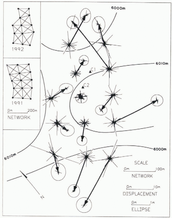
Fig. 3. Stake network at the col of Huascar–n (9– 07° S. 77– 37° W; 6048 m a.s.l.) in the north-central Andes of Peru (Reference ThompsonThompson and others, 1995a). Bold lines with solid arrows are the stake horizontal displacements from September 1991 to September 1992. Displacements are relative to the center of mass of the 1991 positions of the 13 stakes common to the surveys in both years. Because the network could not be connected to bedrock, the motion of the entire array relative to bedrock remains unknown. Ellipsis at end of solid arrows shows the 95% confidence-level error in the displacements. End of the thin lines at base of displacement shows the coordinate shifts that result from marginally delectable blunders in the 1991 observations. Thin lines at tip of displacement arrows show coordinate shifts from mdb in the 1992 observations. Note that one scale is used for the displacement, and another for the ellipsis and shifts from marginally detectable blunders. Locations of cores Cl and C2 are shown as solid triangles. Insets show the stake network in both years where lines represent vectors along which the slant distance and vertical direction relative to adjacent stakes were measured. Solid stake symbols show the stakes common to both surveys.
The stake positions were measured in September 1991 and 1992 using conventional geodetic observations of slant distance and vertical direction from both ends of each line between any two adjacent stakes. These observations were sufficient to determine redundantly the stake positions. To reflect realistic uncertainties for observations collected in the extreme environment of high-altitude ice caps, the assumed observation standard deviations were – (3 mm + 3 ppm) for distances and – 1 cm for instrument heights and centering. In 1991 a subsequent lest of the theodolite revealed a –4.5° of are uncertainty in the vertical directions. In 1992 the instrument was replaced and the vertical directions were observed with a more typical uncertainty of –20° of are.
In neither year could the stake positions be located relative to bedrock, because of a lack of local outcrops. The datum scale and the two orientations in the horizontal plane were defined by the slant-distance and vertical-direction observations. The remaining four datum parameters of azimuthal orientation and three translation components were defined by adopting an inner constraint approach using Equations (35), (39) and (40). Because two of the stakes were not recovered in 1992, the datum for both years was defined by the September 1991 position of the 13 stakes observed in both years.
Figure 4 shows a 600 m – 800 m stake network on the Guliya ice cap (35– 17° N, 81– 29° E; 6200 m a.s.l.) on the Qinghai–Tibetan Plateau that is connected to bedrock through a chain of four braced quadrilaterals that extend about 3.5 km. The network enclosed one drill site from which an ice core of 308.6 m was recovered in 1992 (Reference ThompsonThompson and others, 1995b, Reference Thompson1997). The dense grid at the drill site was spaced at approximately 250 m, and was originally two ice thicknesses wide and five ice thicknesses Song. In 1991, 28 stakes were established of which 19 were recovered in 1992. The stake positions were measured in May 1991 using conventional geodetic observations of slant distance and vertical direction from both ends of each line between any two adjacent stakes and additionally with horizontal directions, with an uncertainty of – 15° of arc, in July 1992. The network extended to bedrock, so the three translational components and the azimuthal orientation were constrained to the e, n and u position of one bedrock point and the azimuth to the other bedrock point.

Fig. 4. Stake network on the Guliya ice cap (35– 17° N, 81– 29° E; 6200 m a.s.l.) on the Qinghai–Tibetan Plateau. Bold lines with solid arrows are the stake horizontal displacements, May 1991–July 1992. Displacements are relative to bedrock points shown as solid squares. Ellipsis at end of solid arrows shows the 95% confidence-level error in the displacements. End of the thin lines at base of displacement shows the coordinate shifts that result from marginally detectable blunders in the 1991 observations. Thin lines with arrows show shifts that exceed 2 m. These result because one diagonal line was not observed in the second quadrilateral west of the bedrock paints. Thin lines at tip of displacement arrows show coordinate shifts from mdb in the 1992 observations. Location of the core (C) is shown as a solid triangle. Insets show the stake network in both years where lines represent vectors along which the slant distance, vertical direction and additionally in 1992 she horizontal direction were measured relative to adjacent stakes. Solid stake symbols show the stakes common to both surveys.
For each of the four observation sets the stake positions, a posteriori coordinate and residual covariances and ![]() were computed (see Table 1). The stake positions were estimated using Equations (35) and (39) at Huascar–n, and (21), (23) and (24) at Guliya. The
were computed (see Table 1). The stake positions were estimated using Equations (35) and (39) at Huascar–n, and (21), (23) and (24) at Guliya. The ![]() was computed using Equation (47), with W = 0 at Huascar–n. The a posteriori covariance of the stake-position estimates was computed at Huascar–n using Equations (42) and (48) and at Guliya using Equations (41) and (48). The a posteriori covariance of the residuals was computed at Huascar–n using Equations (44) and (49) and at Guliya using Equations (43) and (49). In all four adjustments, observations were rejected and removed from the solution if they exceeded the outlier lest given by Equation (51).
was computed using Equation (47), with W = 0 at Huascar–n. The a posteriori covariance of the stake-position estimates was computed at Huascar–n using Equations (42) and (48) and at Guliya using Equations (41) and (48). The a posteriori covariance of the residuals was computed at Huascar–n using Equations (44) and (49) and at Guliya using Equations (43) and (49). In all four adjustments, observations were rejected and removed from the solution if they exceeded the outlier lest given by Equation (51).
The displacement vectors were computed by differencing the coordinate estimates from 1991 and 1992 and are shown in figures 3 and 4. The a posteriori displacement co-variance was computed from the coordinate covariances of each annual survey. The 95% confidence level uncertainty of each displacement estimate is plotted as an ellipse at the tip of the displacement vector in Figures 3 and 4.
The redundancy numbers were computed from Equation (56), the mdb using Equation (57) and coordinate shifts using Equation (59) at Huascar–n and (58) at Guliya. For the 1991 epochs the coordinate shifts at each stake that result from the mdb of each observation are plotted as rays from the 1991 stake location, i.e. the base of the displacement vector. For the 1992 epochs the shifts are plotted as rays from the 1992 stake location, i.e. the tip of the displacement vector. The end-points of the rays represent the location to which the estimated stake location, and thus the base or tip of the displacement vector, could shift due to the mdb.
Discussion
The precision and reliability of surface stake displacements at the Huascar–n and Guliya networks are now examined. Two somewhat arbitrary, but reasonable, criteria are adopted to evaluate the precision and reliability. The precision criterion is that the 95% confidence-level uncertainly in the displacement estimate be less than 10% of the magnitude of the displacement estimate. The reliability criterion is that the potential shifts in the displacement caused by the mdb not exceed the 95% confidence-level uncertainty or be less than 10% of the magnitude of the estimated displacement.
Table 1. Stake network adjustments

The Huascar–n displacement estimate (Fig. 3) at the stake near the center of the network does not meet the precision criterion, but at all other stakes the displacement does meet the precision criterion. From September 1991 to 1992 the estimated displacements range from 0.6 – 0.3 m (2?) near the center of the network to 22.0 – 0.5 m (2?) at the northeast and southwest ends of the network. The displacements are relative to the center of mass of the 1991 positions of the 13 stakes common to the surveys in both years. The relatively large uncertainty in the displacement estimates is due primarily to the –4.5° of are uncertainty in the 1991 vertical direction observations.
The Huascar–n displacement estimate (Fig. 3) at the stake near the center of the network does not meet the reliability criterion, but at all other stakes the displacement does meet the reliability criterion. The potential shifts, due to mdb, in the displacement exceed the 95% confidence-level uncertainty at all stakes, although the potential shifts are less than 10% of the displacement at all stakes except at the center stake. The impact of the mdb on the displacement vector is visualized by recognizing that the base of the displacement vector is free to shift anywhere along the rays plotted at the base. Likewise the tip is free to shift anywhere along the rays plotted at the tip. In 1991, the potential undetectable shifts in estimated positions are as large as –1 m due primarily to the –4.5° of are uncertainty in the 1991 vertical directions. This clearly exceeds the 95% confidence-level uncertainty in the displacement. In 1992, the shifts rarely exceed 20 cm, reflecting the improved precision of the 1992 vertical directions.
The Guliya displacement estimates (Fig. 4) at the stakes near the drill site meet the precision criterion in the east direction, the predominant direction of motion, but fail in the north–south direction. The 95% confidence-level uncertainty in the displacement is computed relative to the bedrock points. At the drill site the 95% confidence-level uncertainty in the displacement approaches –1 m in the north south direction. This reflects the degrading of precision with distance away from the bedrock points, and is predominately in the north–south direction because the geometry and observations control the uncertainty better in the cast-west direction, along the main axis of the network. The uncertainty in the east–west is about –0.25 m and the average displacement approaches 2.7 m, so the precision criterion along the direction of motion is met.
The displacement estimates at the stakes near the drill site do not meet the reliability criterion. Potential coordinate shifts in 1991 from undetected blunders exceed the 95% confidence-level uncertainty. In the second quadrilateral west of the bedrock points, the slant distance and vertical and horizontal direction along one diagonal line were not observed (Fig. 4, inset). This weakens the geometric redundancy of the network. This is only partially reflected in the rather low value ![]() = 0.5 because the usual precision analysis does not sharply depict the lack of geometric redundancy. However, the external-reliability analysis clearly exposes a defect in the network. The small thin tines with arrows plotted from the base of the displacement vectors in Figure 4 show the coordinate shifts that exceed 2 m. In fact some are 10–20 m. Clearly, the farther the points are from the bedrock, the more small errors near the bedrock points are amplified into meter-level errors in the positions of the drill-site network some 3.5 km away. In 1992, inclusion of the missing line and the addition of horizontal directions improved the reliability. Most of the 1992 potential coordinate shifts are within the 95% confidence-level ellipses, but the potential shifts in the displacement are dominated by the 1991 marginally detectable blunders.
= 0.5 because the usual precision analysis does not sharply depict the lack of geometric redundancy. However, the external-reliability analysis clearly exposes a defect in the network. The small thin tines with arrows plotted from the base of the displacement vectors in Figure 4 show the coordinate shifts that exceed 2 m. In fact some are 10–20 m. Clearly, the farther the points are from the bedrock, the more small errors near the bedrock points are amplified into meter-level errors in the positions of the drill-site network some 3.5 km away. In 1992, inclusion of the missing line and the addition of horizontal directions improved the reliability. Most of the 1992 potential coordinate shifts are within the 95% confidence-level ellipses, but the potential shifts in the displacement are dominated by the 1991 marginally detectable blunders.
In general, the Huascar–n and Guliya displacements are perpendicular to the contours of the surface topography.
To the northeast and southwest of the Huascar–n network the ice surface slopes downward. To the north and south the surface slopes upward towards the north and south peaks of Huascar–n. Inflow from the higher regions and outflow to the lower regions appear to explain the general flow pattern seen in the stake displacements. One exception is the eastward motion of one stake on the east side of the network. The precision and reliability analyses indicate there is nothing amiss in the survey observations to explain this motion. Also, the 15–20 m displacements at the northeast and southwest ends of the network are larger than would be expected from the 3.3 m of snow accumulation measured at the stakes from 1991 to 1992 (Reference ThompsonThompson and others, 1995a). The ice dynamics are more complicated than at the dome of a typical ice cap.
At Guliya, the surface slopes gradually upward just west of the bedrock points. The stake displacement from May 1991 to July 1992 varies from approximately 0.15 – 0.05 m (2?) at 750 m west of the bedrock points to an average displacement of 2.7 – 0.5 m (2?) at the drill site, 3.5 km west of the bedrock points. These results represent an improved analysis of the 1991 data using the modeling and statistical tests described in this paper. These results differ from the average of 4.8 m reported in Thompson and others (1995b). For comparison, the accumulation measured during the 1991 and 1992 Geld studies at drill-site stakes was 3.2 m a-1 (1.4 m a-1 water equivalent).
Conclusions
The two examples given used conventional geodetic measurement types in a chain of braced quadrilaterals. At both networks, while the 95% confidence-level uncertainly of the displacement was less than 10% of the displacement, the potential coordinate shifts, due to mdb, exceeded the 95% confidence-level uncertainty of the displacement. At Huascar–n this was primarily due to a –4.5° of are uncertainty in the 1991 vertical directions. At Guliya this was primarily due to a lack of observations along one line. In 1992, at both networks the reliability was significantly improved.
In general, it is possible to meet the precision criterion but have undetected blunders that cause velocity (displacement in time) errors two or more times the magnitude of the velocity precision. To more correctly state the quality of the velocity estimates, the analysis and design should include both precision and internal and external reliability analysis. Fortunately, like precision propagation, the reliability calculations are insensitive to the actual observations, requiring only accurate knowledge of the observation covariance and the approximate geometry permitting a priori analysis.
The GPS observation type was also given and the matrix equations are applicable to GPS observations. The advantage of GPS in defining the network datum, its robust operation in most environments, and the development of small, easy-to-use receivers should eventually replace conventional observations of stake networks accompanying drilling programs on high-altitude remote ice caps.
Acknowledgements
Comments from two anonymous reviewers and the editor significantly improved this paper. L. G. Thompson of the Byrd Polar Research Center (BPRC), Columbus, Ohio, U.S.A., provided the Huascar–n and Guliya surface stake data. W.T. Alegre and J. Greenberg collected the geodetic data. J. F. Bolzan also provided useful comments. This work was initiated while the author was a graduate research assistant at the BPRC.