


Introduction
Along with surface runoff, discharge from marine-terminating outlet glaciers is a primary cause of ice mass loss from the Greenland ice sheet (van den Broeke and others, Reference van den Broeke2009; McMillan and others, Reference McMillan2016). Fast-flowing tidewater glaciers transport volumes of ice from cold, inland regions to warmer coastal areas where it is lost to surface melting submarine melting, and calving (Vieli and Nick, Reference Vieli and Nick2011; Truffer and Motyka, Reference Truffer and Motyka2016). Increasing atmospheric and ocean temperatures have been linked to rapid changes in outlet glaciers including flow acceleration, thinning and rapid retreat (Holland and others, Reference Holland, Thomas, de Young, Ribergaard and Lyberth2008; Moon and others, Reference Moon, Joughin, Smith and Howat2012). Hence, understanding the sensitivity of outlet glaciers to changing climatic conditions is crucial to estimating future mass loss from the Greenland ice sheet.
Evidence suggests that ocean forcing drives retreat of marine-terminating outlet glaciers throughout the Greenland ice sheet (Murray and others, Reference Murray2010; Wood and others, Reference Wood2021). Mechanisms responsible for retreat include increased subaqueous melting caused by intrusion of warm Atlantic waters into fjords (Holland and others, Reference Holland, Thomas, de Young, Ribergaard and Lyberth2008; Rignot and others, Reference Rignot, Koppes and Velicogna2010; Motyka and others, Reference Motyka2011) and turbulent heat exchange at the ice–ocean interface from subglacial discharge (Xu and others, Reference Xu, Rignot, Menemenlis and Koppes2012; Truffer and Motyka, Reference Truffer and Motyka2016). Submarine melt rates can exceed surface melt rates by two orders of magnitude (Truffer and Motyka, Reference Truffer and Motyka2016), and submarine melt accounts for up to 85% of mass loss on floating ice tongues (Enderlin and Howat, Reference Enderlin and Howat2013). Consequently, submarine melt plays an important role in controlling the dynamics of large, marine-terminating glaciers such as Petermann Glacier and Jakobshavn Isbræ in Greenland and Pine Island Glacier in Antarctica (Holland and others, Reference Holland, Thomas, de Young, Ribergaard and Lyberth2008; Jacobs and others, Reference Jacobs, Jenkins, Giulivi and Dutrieux2011; Nick and others, Reference Nick2013).
Another process hypothesized to affect glacier dynamics is decreased basal traction, which produces higher sliding velocities (Zwally and others, Reference Zwally2002). On the Greenland ice sheet, surface velocity can increase during the melt season due to an influx of meltwater into the subglacial drainage system (Joughin and others, Reference Joughin2008; Bartholomew and others, Reference Bartholomew2010; Sundal and others, Reference Sundal2011). This influx of meltwater decouples the bed from the ice, leading to faster basal motion until the subglacial drainage system adapts and pressures decline again (Sundal and others, Reference Sundal2011). Marine-terminating glaciers typically undergo small seasonal speedups of <50%, compared to land-terminating glaciers, which can accelerate by as much as 400% (Joughin and others, Reference Joughin2008; van de Wal and others, Reference van de Wal2008, Reference van de Wal2015; Kehrl and others, Reference Kehrl, Joughin, Shean, Floricioiu and Krieger2017; Davison and others, Reference Davison2020). However, small seasonal changes in velocity still have a significant impact on modeled calving rates (Cook and others, Reference Cook2014). Hence, when the complete seasonal signal is taken into account, mass loss at the glacier front due to calving or submarine melt is affected by basal sliding.
Despite this finding, the significance of basal traction on the mass balance of outlet glaciers is controversial. Thinning of marine glaciers is believed to be primarily a dynamic response to ocean forcing (Sole and others, Reference Sole, Payne, Bamber, Nienow and Krabill2008). Tidewater glaciers exhibit seasonal patterns in thinning rates, terminus position and surface velocity (Moon and others, Reference Moon2014; Kehrl and others, Reference Kehrl, Joughin, Shean, Floricioiu and Krieger2017). Yet, on some tidewater glaciers such as Helheim Glacier and Jakobshavn Isbræ, meltwater-induced seasonal speedups are relatively small (<15%), and large seasonal velocity variations on these glaciers appear to be more closely correlated with seasonal variations in terminus position or floating ice extent rather than surface melting (Joughin and others, Reference Joughin2008b; Andersen and others, Reference Andersen2010; Kehrl and others, Reference Kehrl, Joughin, Shean, Floricioiu and Krieger2017). Modeling studies on Helheim and Petermann glaciers found that traction perturbations resulted in insignificant changes in grounding line position and thickness (Nick and others, Reference Nick, Vieli, Howat and Joughin2009, Reference Nick2012). Similarly, inversions of surface velocity for basal traction suggest basal resistance to flow is very low under fast flowing regions and a more likely control on dynamics is found in the resistance to flow provided by shear-margins (Shapero and others, Reference Shapero, Joughin, Poinar, Morlighem and Gillet-Chaulet2016).
One possible explanation for the diminished role of basal traction in marine-terminating outlet glaciers is that changes at the calving front dominate the dynamical response, reducing the sensitivity of these glaciers to perturbations in basal traction. This explanation leads us to hypothesize that the faster a tidewater outlet glacier is retreating due to ocean forcing, the less sensitive it is to perturbations in basal traction. Basal traction perturbations of a certain magnitude may be drowned out by dynamic changes near the calving front due to submarine melt. Such dynamic changes might include reduced lateral drag due to a retreating calving front, as well as geometric changes that lead to flow acceleration.
To explore the interplay between basal sliding and ocean forcing in greater depth, we perform an ensemble of model experiments using the Ice-sheet and Sea-level System Model (ISSM), a finite-element-based, thermo-mechanically coupled ice-sheet model (Larour and others, Reference Larour, Seroussi, Morlighem and Rignot2012). We first construct a time-dependent model of Upernavik Isstrøm, a large, marine-terminating outlet glacier system in northwest Greenland.
Since the earliest direct observations in 1849 (Weidick, Reference Weidick1963), Upernavik Isstrøm has retreated 20–30 km, rivaling the retreat of some of Greenland's most prominent outlet glaciers such as Jakobshavn Isbræ (~ 40 km). Over the past several decades, Upernavik Isstrøm has experienced substantial, dynamic mass loss due to flow acceleration and thinning (Haubner and others, Reference Haubner2018). Between 2001 and 2007, the mean submarine melt rate at the northernmost trunk of Upernavik Isstrøm was estimated at 1.83 m d−1, which was higher than 9 of the 13 other Greenland tidewater glaciers in Enderlin and Howat (Reference Enderlin and Howat2013). The high rate of subaqueous melting suggests that Upernavik Isstrøm has undergone ocean-forced retreat, making it an ideal setting for our numerical experiments.
The numerical model is allowed to reach a steady state under constant climate and ocean forcing. Initialized from this steady state, a variety of retreat scenarios are simulated by forcing the model with different submarine melt rates and basal traction perturbations. We analyze the results of these runs in order to understand how the modeled response to basal-sliding perturbations depends on the subaqueous melt rate.
Methods
Model
To model ice dynamics in Upernavik Isstrøm, we use the ISSM (Larour and others, Reference Larour, Seroussi, Morlighem and Rignot2012). We use an anisotropic computational mesh with a resolution ranging from 200 m near the grounding line to 1333 m in the ice-sheet interior (Fig. 1). Ice velocity is modeled using the shallow-shelf approximation (MacAyeal, Reference MacAyeal1989). Ice flux is constrained on the inland (eastern) boundary of Upernavik Isstrøm, while ice velocity is constrained on the lateral boundaries. Basal sliding follows a Budd-like sliding law (Budd and others, Reference Budd, Keage and Blundy1979)

where τb is the basal stress, N is effective pressure, u is basal velocity and $\beta _0^{2}$ is a basal friction coefficient determined by inverting for surface velocity. Here, effective pressure is defined by

where P i is the ice overburden pressure and P w is the subglacial water pressure. Water pressure is a function of bedrock elevation, transitioning smoothly from sea level water pressure in the fjord, where we assume a strong hydraulic connection to the ocean, to a fixed fraction of ice overburden pressure (85%) in regions where the bed is above sea level. Water pressure takes the form
where P sea is the sea level water pressure and f P is an indicator function of the form
where z b is the bed elevation and ℓ is a parameter tuned such that f P transitions smoothly from 0 to 1 over a length scale of around a kilometer.
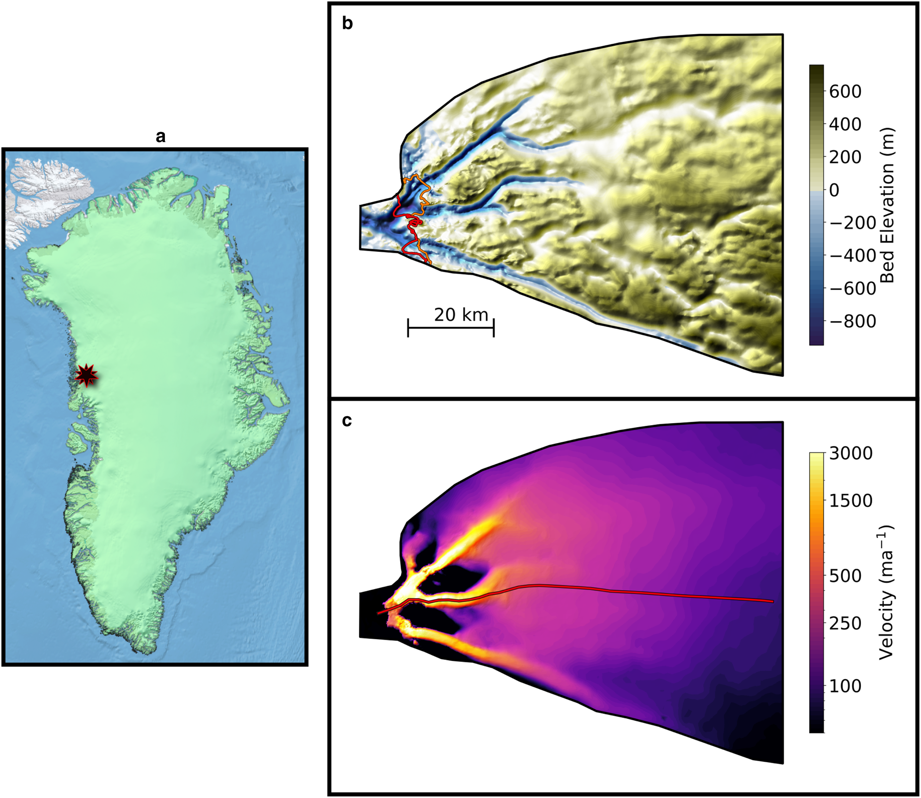
Fig. 1. (a) Location of the Upernavik Isstrøm glacier complex in western Greenland. (b) Bed elevation data on computational domain. Red and orange lines indicate steady-state terminus and grounding lines, respectively. (c) Steady-state ice velocity used in all numerical experiments. The red line indicates a flowline along the central trunk of Upernavik Isstrøm used for the analysis in Figures 5 and 6. Velocity is constrained on the lateral and right edges to the average velocity between 1985 and 2018 from the ITS_LIVE project (Gardner and others, Reference Gardner2018) and flux is constrained on the right edge using thickness from Bedmachine v3 (Morlighem and others, Reference Morlighem2017).
We use the von Mises stress calving law available in the ISSM to determine the calving rate at the glacier front (Morlighem and others, Reference Morlighem2016). Calving rate c is given by

where σ max is a calibrated stress threshold and $\tilde {\sigma }$ is the tensile von Mises stress. We have

where B is the ice hardness and n = 3 is Glen's exponent. The effective tensile strain rate $\tilde {\dot {\epsilon }}_{\rm e}$ is defined by
where $\dot {\epsilon _1}$ and $\dot {\epsilon _2}$
 represent the eigenvalues of the 2-D horizontal strain rate vector. We tune the stress threshold σ max to 825 kPa based on the value inferred for the northern trunk of Upernavik Isstrøm in Choi and others (Reference Choi, Morlighem, Wood and Bondzio2018). Sensitivity testing indicates that our model results are qualitatively insensitive to this parameter value.
Bed and surface elevation data for Upernavik Isstrøm are obtained from Bedmachine v3 (Morlighem and others, Reference Morlighem2017) (Fig. 1a). We use yearly averaged surface mass balance from RACMO (Noël and others, Reference Noël, Berg, Lhermitte and Broeke2019) and average surface velocity between 1985 and 2018 from the ITS_LIVE project as boundary conditions and to constrain basal traction (Gardner and others, Reference Gardner, Fahnestock and Scambos2021). Following Nick and others (Reference Nick2012) we use a spatially varying, vertically averaged ice hardness field corresponding to the steady-state ice temperature. To solve for ice temperature, we use a 30 year average of near surface air temperature from 1980 to 2010 at the surface boundary (Box, Reference Box2013) and a uniform geothermal heat flux of 70 mW m−2 at the ice base.
Model experiments
We perform 99 model runs testing different basal traction and submarine melt rate combinations. All model runs are initialized from a steady state generated by running the model with stable climate and ocean forcing. We find that using an annual surface mass balance (SMB) field from 1990 combined with a subaqueous melt rate of 0.4 m d−1 yields a steady-state glacier with an extent slightly greater than modern Upernavik Isstrøm. While our objective is not to reconstruct the historical retreat of Upernavik Isstrøm, we note that modeled SMB is representative of climatic conditions during the time period 1964–1990, during which SMB remained stable (Haubner and others, Reference Haubner2018). Beginning from this equilibrium state, an ensemble of retreat scenarios are simulated by instantaneously setting the subaqueous melt rate to values ranging from 0.4 to 2.4 m d−1. This is intended to simulate an increase in subaqueous melting, potentially caused by intrusion of warm Atlantic water into Upernavik icefjord. Subaqueous melt is applied uniformly to the base of floating ice. We find that melting on the underside of floating ice tongues dominates the dynamics of Upernavik Isstrøm, and find the model insensitive to the frontal melting or undercutting rate in the ISSM.
All model runs are 50 years in length. After 25 years of simulation time, when the glacier is retreating due to ocean forcing, the basal traction coefficient is reduced by a fixed percentage ranging from 0 to 40%. This perturbation is intended to roughly simulate an interannual increase in basal sliding caused by increasing surface melt input to the bed or a longer melt season duration. In particular, the basal traction coefficient is given by

The baseline basal traction coefficient $\beta _0^{2}( x,\; \, y)$ was determined by inverse modeling (Morlighem and others, Reference Morlighem2010) using the ITS_LIVE surface velocities with Bedmachine v3 ice geometry. Here, f(x, y) is a smoothed indicator function that has a value of ~1 in areas where the SMB $\dot {a}( x,\; \, y)$
 is negative and ~0 where it is positive:

The parameter 0 ≤ p ≤ 0.4 controls the reduction in basal traction, which ranges from 0 to 40%. The temporal scaling function s gradually activates the basal traction perturbation midway through each 50 year simulation and is given by

In order to isolate the impact of subaqueous melt and basal traction perturbations, the SMB is kept static throughout each model run.
To test sensitivity of the results to the sliding law, we performed 55 additional model runs using a nonlinear sliding law of the form

Here, we solve for the basal traction coefficient $\beta _0^{2}$ such that steady-state basal drag is identical for both the linear and nonlinear sliding laws.
Results
Modeled ice mass loss from Upernavik Isstrøm displays a nonlinear relationship with the subaqueous melt rate. Upernavik Isstrøm remains relatively stable for melt rates between 0.4 and 1 m d−1. In this range, Upernavik Isstrøm loses a maximum of ~150 Gt of mass over 50 years (Figs 2a, d), and both subaqueous melting and basal traction perturbations are important for determining total mass loss (Fig. 2c). In contrast, melt rates exceeding 1 m d−1 yield rapid thinning and grounding-line retreat, irrespective of traction perturbations (Fig. 3). For the maximum tested subaqueous melt rate of 2.4 m d−1 and a basal traction coefficient reduction of 40%, Upernavik Isstrøm loses over 500 Gt of ice, which is ~0.06% of its steady-state mass (Fig. 2a).
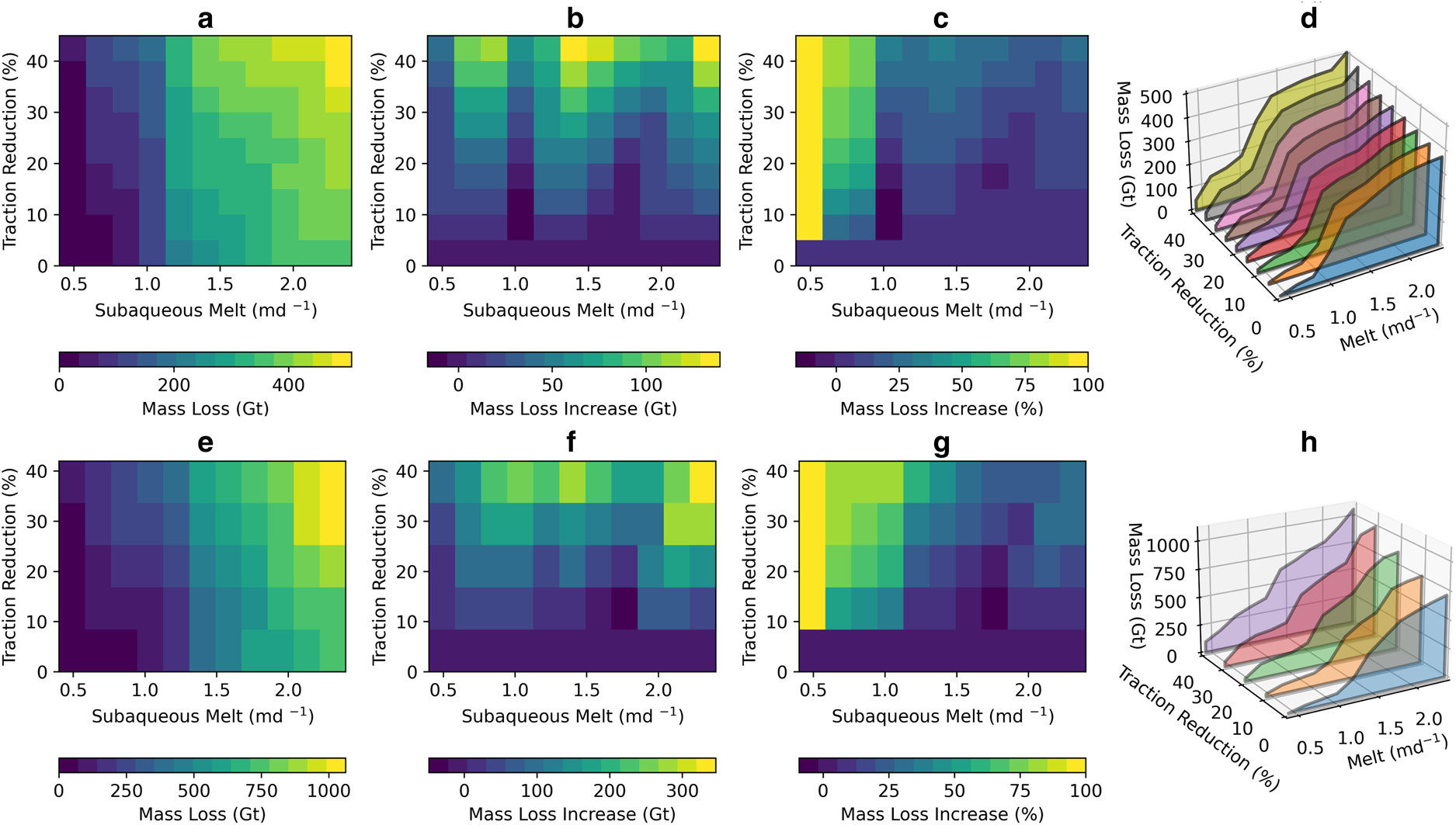
Fig. 2. (a) Gigatons of ice mass loss from Upernavik Isstrøm after 50 years for an ensemble of model runs with subaqueous melt values ranging from 0.4 to 2.4 m d−1 and basal traction reductions ranging from 0 to 40%. Each column in (b) shows the additional mass lost due to reduced basal traction compared to a baseline run with the same subaqueous melt rate and no basal traction perturbation. Panel (c) shows the percentage increase in mass loss caused by basal traction reductions versus a model run with the same subaqueous melt but no basal traction perturbation. (d) Alternative view of panel (a) showing gigatons of mass loss for various parameter combinations. Panels (e), (f), (g), (h) show equivalent metrics to panels (a), (b), (c), (d), respectively, for the experiment using a nonlinear sliding law.
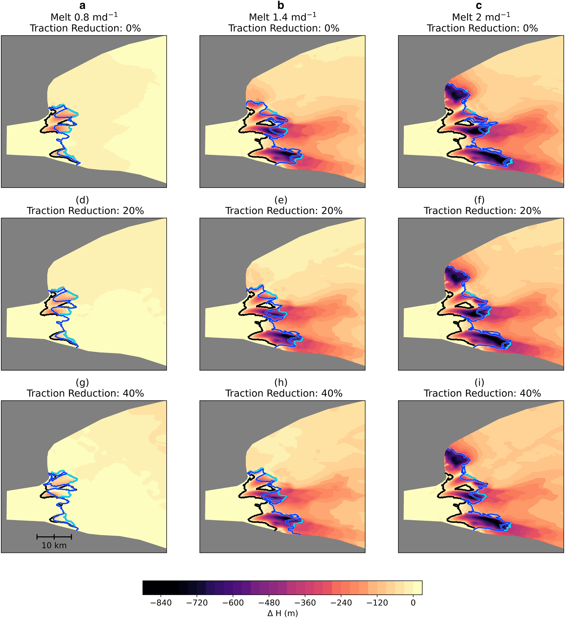
Fig. 3. Thinning of Upernavik Isstrøm for simulations with subaqueous melt rates ranging from 0.8 to 2 m d−1 combined with basal traction reductions from 0 to 40%. The black line shows the initial terminus position, while dark and light blue lines show the final terminus position and grounding line at the end of each simulation, respectively.
We compute the additional mass loss from enhanced sliding by comparing mass loss in runs with perturbed basal traction coefficients to a run with the same melt rate and no traction perturbation. Reducing the basal traction coefficient β2 by up to 40% results in anywhere from 45 to 140 Gt of additional mass loss, depending on the subaqueous melt rate (Fig. 2b). Additional mass loss increases roughly linearly with the parameter p in Eqn (8), which represents the percent reduction in the traction coefficient. Mass loss from basal traction behaves unpredictably as a function of the subaqueous melt rate. Hence, there is not a clear trend between higher subaqueous melt rates and reduced sensitivity to basal traction perturbations as hypothesized.
However, if we consider losses from enhanced sliding as a fraction of the total mass loss, we see a somewhat different picture. In particular, there is an abrupt transition from relatively balanced mass loss from enhanced sliding and subaqueous melting to predominantly submarine melt-driven mass loss around a subaqueous melt rate of 1 m d−1. Below this threshold, traction reductions have an important influence on overall mass loss, and traction coefficient reductions of 40% yield at least 75% additional mass loss (Fig. 2c). Yet, above this 1 m d−1 threshold, traction perturbations account for <35% of the total mass loss for all tested traction perturbations. Hence, basal traction perturbations are less important, relatively speaking, for higher melt rates.
We can assess our hypothesis more directly by examining gradients of mass loss with respect to basal traction perturbations. For a given melt rate, the sensitivity of the model to basal traction perturbations is given by the gradient of mass loss with respect to the percent reduction in basal traction, averaged over all tested traction perturbations. Sensitivity varies widely for different subaqueous melt rates, with peaks in sensitivity at 0.8, 1.4 and 2.4 m d−1 and troughs at 0.4, 1 and 2.2 m d−1 (Fig. 4a). Thus, contrary to our hypothesis, higher melt rates do not generally correspond to lower sensitivity to basal traction reductions.
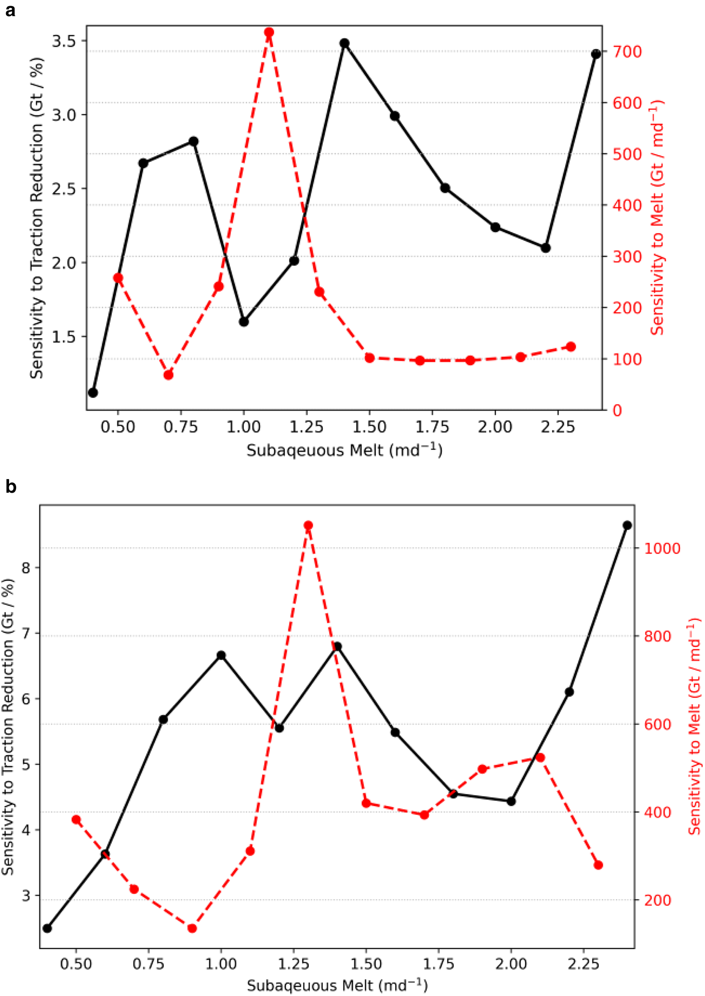
Fig. 4. (a) Average sensitivity of total mass loss to basal traction reductions (black line) and subaqueous melt (red line) for different subaqueous melt rates. Sensitivities are computed by averaging the gradient of mass loss with respect to the percent reduction in the basal traction reduction or to the subaqueous melt rate, averaged over all basal traction perturbations. Note the different scales for traction/subaqueous melt sensitivities. (b) Sensitivities for a similar experiment using a nonlinear sliding law.
High subaqueous melt rates yield rapid grounding-line retreat and thinning localized near the glacier front (Fig. 3). In contrast, since basal traction perturbations cause flow acceleration over a broad area, they can cause thinning deeper into the interior. While basal traction perturbations cause increased mass loss, they do not necessarily cause grounding-line retreat (e.g. Figs 3b, e, h). This is because ice lost near the glacier front due to submarine melting and calving is rapidly replaced by increased ice flux from upstream caused by faster sliding.
Submarine melting and enhanced sliding yield different spatial changes in ice surface velocity. Subaqueous melt exerts the main control on velocity near the grounding line. On the central trunk of Upernavik Isstrøm, melt rates exceeding 1 m d−1 cause rapid thinning at the glacier front, which results in a more than twofold increase in velocity averaged within 15 km of the grounding line (Figs 5b, c). About 30–45 km into the interior, the velocity signal from subaqueous melting is nearly indiscernible, but traction coefficient perturbations produce speedups of up to 50% (Figs 5h, i).
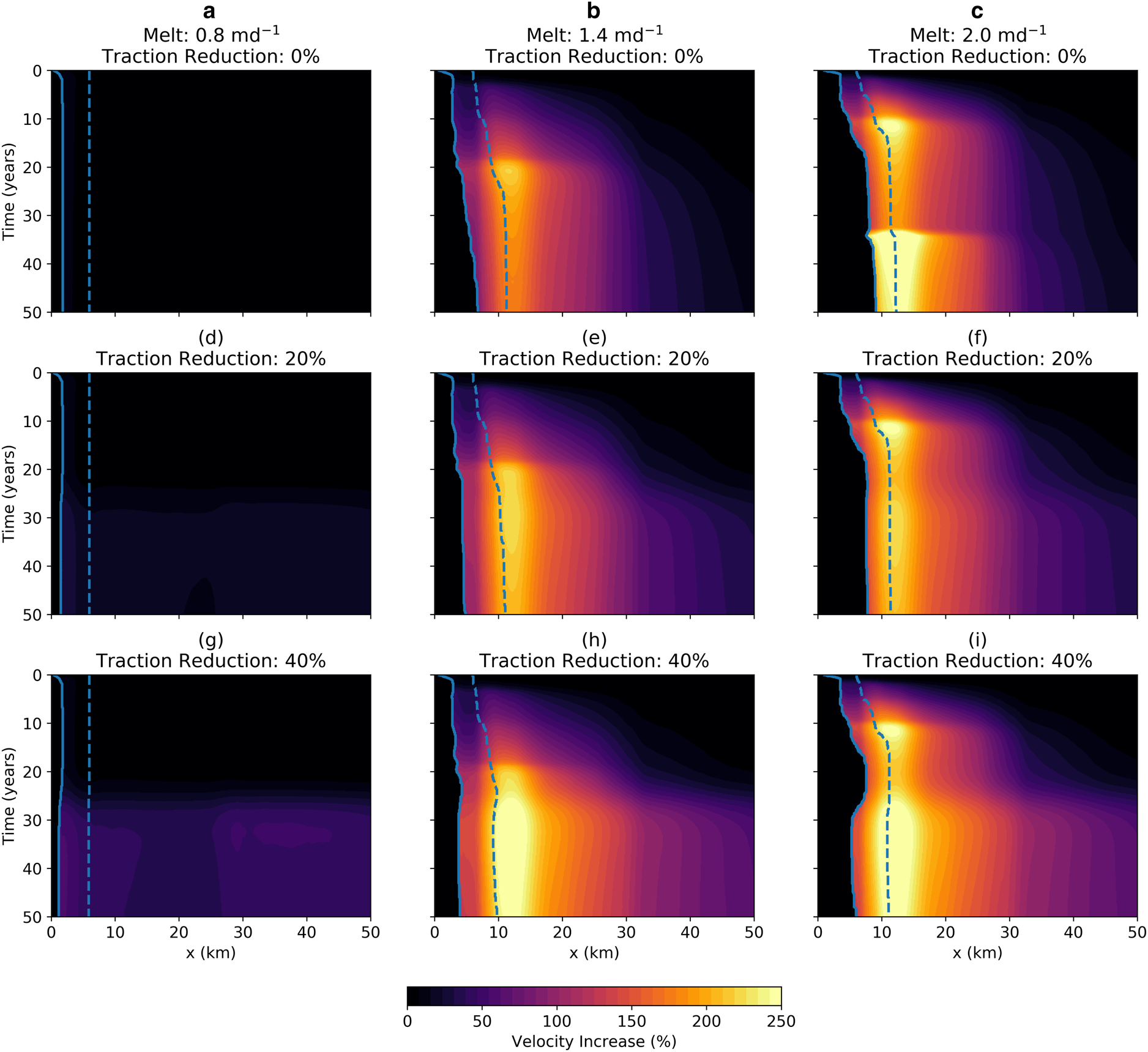
Fig. 5. Percent increase in velocity along the central trunk of Upernavik Isstrøm (Fig. 1b) over 50 years for runs with different parameter values. Columns show simulations with subaqueous melt rates of 0.8, 1.4 and 2 m d−1 (from left to right respectively). Rows show basal traction coefficient reductions of 0, 20 and 40% (top to bottom respectively). Solid and dashed blue lines show the terminus and grounding line positions, respectively.
Recording the peak percentage increase in velocity within three regions of the glacier complex shows that the lower 15 km experiences a much greater acceleration than regions further from the terminus (Fig. 6). When the results are displayed this way, in the lower region we see a discontinuity in the response near a 1.0 m d−1 threshold in subaqueous melt. This discontinuity was previously noted when considering results displayed in Figures 2 and 5. Maximum velocity increases deeper in the interior (Figs 6b, c) are subdued, suggesting that the marine signal has dissipated at this point and responses are more strongly governed by the perturbation to basal traction.
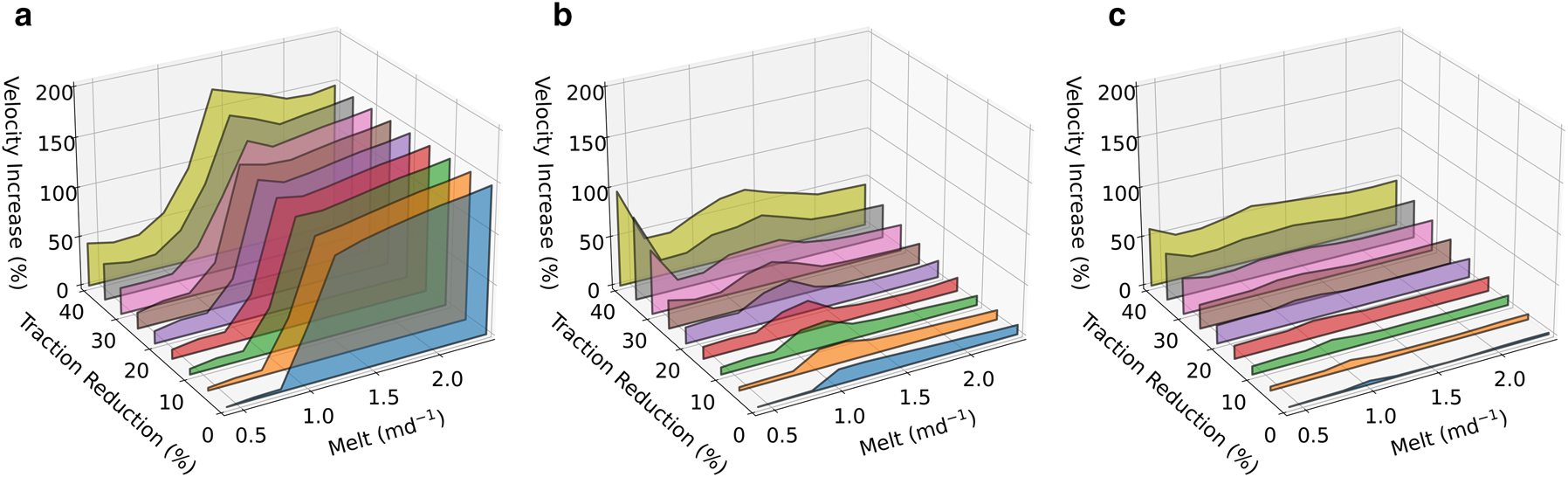
Fig. 6. Peak increase in surface velocity for different subaqueous melt rates and traction reductions. Panels (a), (b) and (c) show the peak increase in average velocity for regions 0–15, 15–30 and 30–45 km inland of the grounding line, respectively, on the central trunk of Upernavik Isstrøm.
Qualitatively, mass loss trends are similar for both the linear and nonlinear sliding laws, with a few key differences. For the nonlinear sliding law, we observe a similar, but less marked nonlinearity in mass loss with respect to the subaqueous melt rate around a melt rate of 1.2 m d−1 (Figs 2e, g). Overall mass loss in the nonlinear experiments is much greater. For example, for a submarine melt rate of 2.4 m d−1 and traction coefficient reduction of 40%, Upernavik Isstrøm loses around double the mass using the nonlinear sliding law than the linear sliding law. This is primarily due to an increased sensitivity to basal traction perturbations (Fig. 4b). Although mass loss is still dominated by submarine melting for higher submarine melt rates, traction perturbations cause around three times as much mass loss compared to the linear sliding law (Fig. 2f).
Discussion
Our experiments on Upernavik Isstrøm reveal complex interactions between subaqueous melting and basal sliding that control modeled glacier mass loss. Modeled mass loss displays a nonlinear relationship with the subaqueous melt rate. We can generally characterize Upernavik Isstrøm as stable for melt rates below 1 m d−1, while higher rates induce significant ocean-forced grounding-line retreat, thinning and surface velocity acceleration (Figs 3, 5). This results in a transition from mixed mass loss from both submarine melting and enhanced sliding to predominantly subaqueous melt caused mass loss around a submarine melt rate threshold of 1 m d−1 (Fig. 2c).
On the central trunk of Upernavik Isstrøm, melt rates exceeding 1 m d−1 induce an up to 175% increase in velocity averaged within 15 km upstream of the grounding line (Fig. 6a). This acceleration is broadly consistent with satellite observations of velocity between 1985 and 2018 (Gardner and others, Reference Gardner, Fahnestock and Scambos2021), a period in which Upernavik Isstrøm may have undergone ocean-forced retreat. Further inland, velocity is less sensitive to submarine melting, but basal traction reductions can cause significant speedups. Hence, 15–45 km into the interior, basal traction reductions of up to 40% can cause speedups of up to 50% above the steady-state ice velocity.
Observations show that tidewater glaciers undergo distinct seasonal velocity cycles, including early melt season acceleration of up to 40% (e.g. Davison and others, Reference Davison2020). This seasonal cycle is thought to be modulated by the evolution of the subglacial drainage system as it adapts to changes in meltwater input. It is difficult to contrast observed seasonal speedups on marine outlet glaciers with the interannual speedups considered in our model experiments. Indeed, our study is limited in the sense that we do not model subglacial hydrology or account for seasonal variations in basal sliding. Nonetheless, our results suggest that modest seasonal speedups, as well as interannual speedups that could result from increased surface melting, are secondary to processes at the glacier front when it comes to predicting future mass loss from tidewater outlet glaciers. While enhanced basal sliding causes considerable mass loss irrespective of the submarine melt rate, it accounts for a relatively small fraction (≈25%) of the total loss when Upernavik Isstrøm is rapidly retreating due to subaqueous melting (Fig. 2c).
Our results are important as finite resources are deployed to monitor the Greenland ice sheet and other rapidly evolving components of the cryosphere. If it is the case that marine-terminating glaciers in rapid retreat are less sensitive to basal perturbation in the force balance, then detailed observations upstream are less important, and efforts can be redirected to the terminus without a loss in fidelity. On the other hand, if the perturbations are additive, and outlet glaciers are accelerating in response to changes at both the marine terminus and the bed, another, more holistic set of priorities for study occurs. Consider, for example, that for a submarine melt rate of 1.8 m d−1, which is approximately the average rate inferred for the northern trunk of Upernavik Isstrøm between 2001 and 2007 (Enderlin and Howat, Reference Enderlin and Howat2013), a 40% reduction in the basal traction coefficient causes an ~40% increase in the annual flow velocity averaged 15–45 km upstream of the grounding line on the central trunk of Upernavik Isstrøm. Since this refers to an increase in annual rather than merely seasonal velocity, the mass loss associated with this traction reduction is likely greater than would be expected from a transient summer speedup of 40% over the same region. Despite this, it is associated with only a 20% increase in mass loss. Therefore, processes at the glacier front are of primary importance for estimating mass loss.
For higher melt rates, Upernavik Isstrøm's floating ice tongues shrink considerably after 50 years (Figs 1, 3), which in turn reduces sensitivity to the subaqueous melt rate beyond a threshold of ~1.2 m d−1 (Fig. 4). Yet, even as floating tongues shrink, subaqueous melt still features significantly in ice dynamics. Not only does submarine melt cause direct mass loss, it also facilitates calving by thinning floating ice. It is possible that, given a longer simulation time, further shrinking of ice tongues would eventually diminish the significance of subaqueous melting. However, we do not witness this on the half-century timescale in our simulations. In tandem with submarine melt, enhanced basal sliding increases ice flux into the fjords where, once afloat, it thins due to submarine melting and eventually calves into the ocean. We see an interesting example of the interplay between basal traction perturbations and calving in model runs with high melt rates and large basal traction reductions. Perhaps, counterintuitively, faster basal sliding does not cause significant grounding-line retreat, as ice loss near the glacier front is replenished by high flux of ice from the interior. That is, the grounding line does not thin appreciably because upstream acceleration transports enough ice to the grounding-line region to offset thinning and acceleration there.
Recent studies such as Joughin and others (Reference Joughin, Smith and Schoof2019) and Åkesson and others (Reference Åkesson, Morlighem, O'Regan and Jakobsson2021) have emphasized the importance of the sliding law in determining modeled mass loss. Åkesson and others (Reference Åkesson, Morlighem, O'Regan and Jakobsson2021) compared grounding-line retreat and sea-level-rise for Petermann Glacier using several sliding laws including a Budd-like law of the form used here, as well as a till friction law (Seguinot and others, Reference Seguinot, Rogozhina, Stroeven, Margold and Kleman2016) and a Schoof friction law (Schoof, Reference Schoof2005). They noted vastly different rates of sea level rise depending on the sliding law. Although testing the sensitivity of mass loss across different sliding laws is not a primary goal of this study, we found that a nonlinear sliding law exhibited greater overall mass loss and higher sensitivity to traction coefficient perturbations due to lower basal drag at high velocities. Nonetheless, certain features are consistent between the linear and nonlinear friction laws. In both cases, we see a nonlinear response of mass loss to the subaqueous melt rate at 1 m d−1 in the linear law and 1.2 m d−1 for the nonlinear law (Figs 2d, h). We also see a roughly inverse relationship between sensitivity to subaqueous melt and traction coefficient perturbations (Figs 4a, b). We acknowledge that the simplistic Budd-like sliding relation is known to produce distinctive patterns of velocity that may not be consistent with observation (Joughin and others, Reference Joughin, Smith and Schoof2019). Sliding relations that provide a bound on basal traction, such as the till or Schoof friction laws mentioned above, may do a better job of reproducing observations of marine-terminating glaciers (Joughin and others, Reference Joughin, Smith and Schoof2019).
Although we are interested in understanding the general behavior of Greenland's marine-terminating glaciers, our model results depend on the particular bedrock geometry of the Upernavik Isstrøm region. For marine-terminating outlet glaciers, thinning initiated at the glacier front propagates up-glacier, and the extent of upstream thinning is controlled by the underlying bedrock geometry (Felikson and others, Reference Felikson2017, Reference Felikson, Catania, Bartholomaus, Morlighem and Noël2021). Bedrock geometry therefore influences how much mass is lost due to ocean forcing. In the absence of basal traction perturbations, we find that thinning caused by subaqueous melting is restricted to an area within ~40 km inland of the steady-state terminus position. Bedrock elevation increases up-glacier along the fjords underlying the primary trunks of Upernavik Isstrøm, which likely limits the extent of ocean-forced thinning.
It is likely that the complex, nonlinear response of mass loss with respect to subaqueous melt is modulated at least in part by bedrock geometry. Differences in the linear and nonlinear sliding laws also indicate the important role of ice dynamics. The nonlinearity ~1 m d−1 depends on feedbacks between submarine melt, basal sliding and calving on the complex bed geometry of Upernavik Isstrøm. One possible explanation is that above this threshold, submarine melting causes enough thinning at the glacier front to cause significant ice acceleration and therefore mass loss. This could perhaps be a kind of debutressing effect, where thinning at the glacier front reduces backstress on the upstream part of the glacier. However, it is not clear why this threshold exists. Indeed, for the nonlinear sliding experiments, this instability appears to occur at a slightly higher melt rate, which means that this threshold is dependent on ice dynamics.
Submarine melting varies as a function of time, location and depth (Xu and others, Reference Xu, Rignot, Fenty, Menemenlis and Flexas2013; Truffer and Motyka, Reference Truffer and Motyka2016; Rignot and others, Reference Rignot2016). Andersen and others (Reference Andresen, Kjeldsen, Harden, Norgaard-Pedersen and Kjaer2014) found that below 150 m in the water column, the water in the Upernavik icefjord gradually warms to 3°C. In comparison with other modeling studies that account for these temporal and spatial variations in the submarine melt rate (e.g. Nick and others, Reference Nick2012; Choi and others, Reference Choi, Morlighem, Rignot and Wood2021), we use a simplified treatment by applying a uniform melt rate across the base of floating ice. This simplification is justified in our case as we are primarily interested in exploring the sensitivity of Upernavik Isstrøm to basal traction perturbations under conditions of ocean-forced retreat. Hence, we are examining broad trends in mass loss across a large range of possible mean melt rates, rather than modeling Upernavik Isstrøm as accurately as possible. We do not expect that this simplification plays an important role in our findings.
Ultimately, we find greater complexity in Upernavik Isstrøm than hypothesized. Our results show the system is sensitive to perturbations in basal traction across the entire range of subaqueous melt rates. From this, we reject our initial hypothesis that the glacier is less sensitive to basal traction perturbations when undergoing ocean-forced retreat. However, the sensitivity varies in ways we did not anticipate. Diminished sensitivity occurs at melt rates of 0.4, 1 and 2.2 m d−1 and high sensitivities at 0.8, 1.4 and 2.4 m d−1. These intermittent regions of lower sensitivity correspond to regions where the sensitivity to subaqueous melt increases (Fig. 4). This suggests a refined hypothesis that marine glaciers are sensitive to changes in both the subaqueous melt and the basal traction, but that their sensitivities operate in inverse proportion to one another. However, our results cannot adequately test this refined hypothesis without additional experimentation.
Our approach follows a line of inquiry that relates glacier response to state and has been productive in defining large scale instabilities (Weertman, Reference Weertman1974; Schoof, Reference Schoof2007; Pollard and others, Reference Pollard, DeConto and Alley2015) that may lead to abrupt and catastrophic change. We observe that instabilities such as the marine-ice or ice-cliff instabilities are characterized by unique geometric states. In this study, we have experimented with particular, far from equilibrium states that are defined by the velocity, rather than the position of the ice mass. While nothing encountered in this study could be considered an instability, it is worth pointing out that there may be states in the ice sheet's momentum that are more (or less) sensitive to perturbations and merit further study. We are not aware of other study suggesting or acting on this idea, and that contributes to the novelty of this study.
Conclusion
In this study, we characterized a marine-terminating glacier's state-dependent response to perturbations in basal traction. The glacier's state was varied by imposing subaqueous melt at the marine boundary, which drove grounding-line retreat. Responses showed state dependence, but not in the anticipated way; while ocean-forcing was the primary driver of mass loss in most simulations, a rapidly retreating glacier was not necessarily less sensitive to perturbations in basal traction than one closer to equilibrium. We found that, for the linear sliding law, high subaqueous melt rates caused significant mass loss and acceleration localized near the ice front, whereas basal traction reductions caused acceleration and thinning deeper into the interior. Our experiments showed a highly nonlinear response of mass loss to the subaqueous melt rate around a threshold of ~1 m d−1. It is likely that this nonlinearity is modulated by the interplay between basal sliding, subaqueous melting and calving on the complex fjord geometry of Upernavik Isstrøm. Experiments using both linear and nonlinear sliding laws differed in terms of the amount of mass lost and the sensitivity to basal traction perturbations. Using a nonlinear sliding law yielded roughly double the mass loss, and while subaqueous melt was still the dominant driver of mass loss, we found the model to be more sensitive to basal traction perturbations. Despite these differences, both sliding laws suggest that there may be an inverse relationship in sensitivity to subaqueous melt and basal traction perturbations for marine-terminating glaciers.
Acknowledgements
J. Z. Downs and J. V. Johnson were supported by NSF grant 1543533. The authors sincerely thank Mathieu Morlighem for help using ISSM to conduct the model experiments presented in this study. The authors also thank Joel Haper and Toby Meirbachtol for insightful discussions that aided in the development of this study. Additionally, the authors thank editor Frank Pattyn as well as Trevor Hillebrand and another anonymous reviewer for their help improving the manuscript.


 Open access