


1. Introduction
Ice rises are locally grounded regions within ice shelves that provide a stabilizing resistance to ice flow (Thomas and others, Reference Thomas1979; MacAyeal and others, Reference MacAyeal, Bindschadler, Stephenson, Shabtaie and Bentley1987; Favier and Pattyn, Reference Favier and Pattyn2015; Matsuoka and others, Reference Matsuoka2015). Model experiments have shown that ice rises can stabilize grounding lines in otherwise unstable configurations (Goldberg and others, Reference Goldberg, Holland and Schoof2009). However, ice rise formation and evolution are currently poorly understood (Matsuoka and others, Reference Matsuoka2015), and many ice rises are too small to be resolved by continent-scale ice-sheet models. Observation-based understanding of ice rise processes is necessary to accurately parameterize them in ice-sheet models. Here we present new observations that provide insight into the formation and evolution of an ice rise.
Crary Ice Rise (CIR) is a grounded promontory within the Ross Ice Shelf (Fig. 1) that provides roughly half the resistance to flow from Whillans and Mercer Ice Streams, and reduces ice-shelf spreading rates by an order of magnitude (MacAyeal and others, Reference MacAyeal, Bindschadler, Stephenson, Shabtaie and Bentley1987, Reference MacAyeal, Bindschadler, Stephenson, Shabtaie and Bentley1989; Still and others, Reference Still, Campbell and Hulbe2018). Along with Roosevelt Island and Steershead Ice Rise, it is one of only three ice rises identified within the Ross Ice Shelf (Matsuoka and others, Reference Matsuoka2015). Streak lines and rifts visible on the surface of the ice shelf indicate the ice rise has existed for at least 700 years (Fahnestock and others, Reference Fahnestock, Scambos, Bindschadler and Kvaran2000). Borehole thermometry data and thermal modeling indicate that the ice rise formed in at least two stages, when the ice shelf re-grounded ~1 kyr and ~600 yr BP (Bindschadler and others, Reference Bindschadler, Roberts and Iken1990). It is not known whether the re-grounding was a result of increased discharge from the Siple Coast ice streams (Bindschadler, Reference Bindschadler1993), isostatic rebound (e.g. Kingslake and others, Reference Kingslake2018) or a combination of the two. While two stages have been identified in the evolution of CIR (Bindschadler and others, Reference Bindschadler, Roberts and Iken1990), the Siple Coast ice streams have stagnated and reactivated multiple times over the last millennium (Catania and others, Reference Catania, Hulbe, Conway, Scambos and Raymond2012). Thus, it is likely that the formation and evolution of CIR was more complex than has been demonstrated to this point. Here we use new ground-based radio-echo sounding data to map englacial structures and stratigraphy to interpret the dynamics of grounding and subsequent evolution of the ice rise. We then model radar waveforms to test hypotheses about the origin of the radar-detected structures we observe.
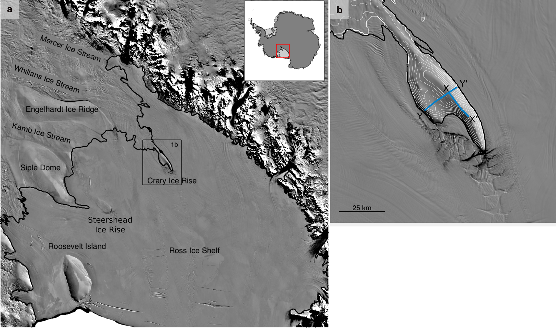
Fig. 1. Location of Crary Ice Rise in the Ross Embayment of Antarctica. Tracks of the two main radar surveys discussed are shown in Figure 1b. Annotated echograms from the surveys are shown in Figures 2, 3. The 10 m elevation contours from Fretwell and others (Reference Fretwell2013) are shown in white to give an indication of flow direction for grounded ice. Maps generated using the Antarctic Mapping Toolbox for MATLAB (Greene and others, Reference Greene, Gwyther and Blankenship2017).
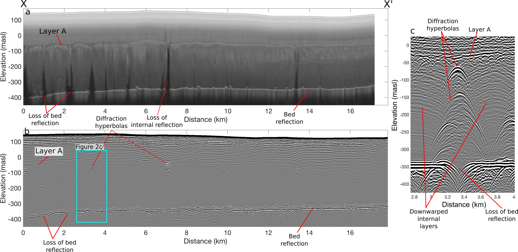
Fig. 2. Transect X–X’ along the crest of the main ridge of the ice rise using radars operating at 750 MHz (a) and 7 MHz (b). Both echograms are corrected for surface topography. The 750 MHz data were processed using the CReSIS toolbox. The 7 MHz data are not migrated so as to reveal the diffraction hyperbolas. Layer A and several examples of diffraction hyperbolas and loss of bed or internal reflections are labeled. (c) Enlarged section of profile X–X’, shown by the cyan box in (b). Note the down-warping of internal layers toward the stacks of diffraction hyperbolas, accompanied by loss of bed reflection.
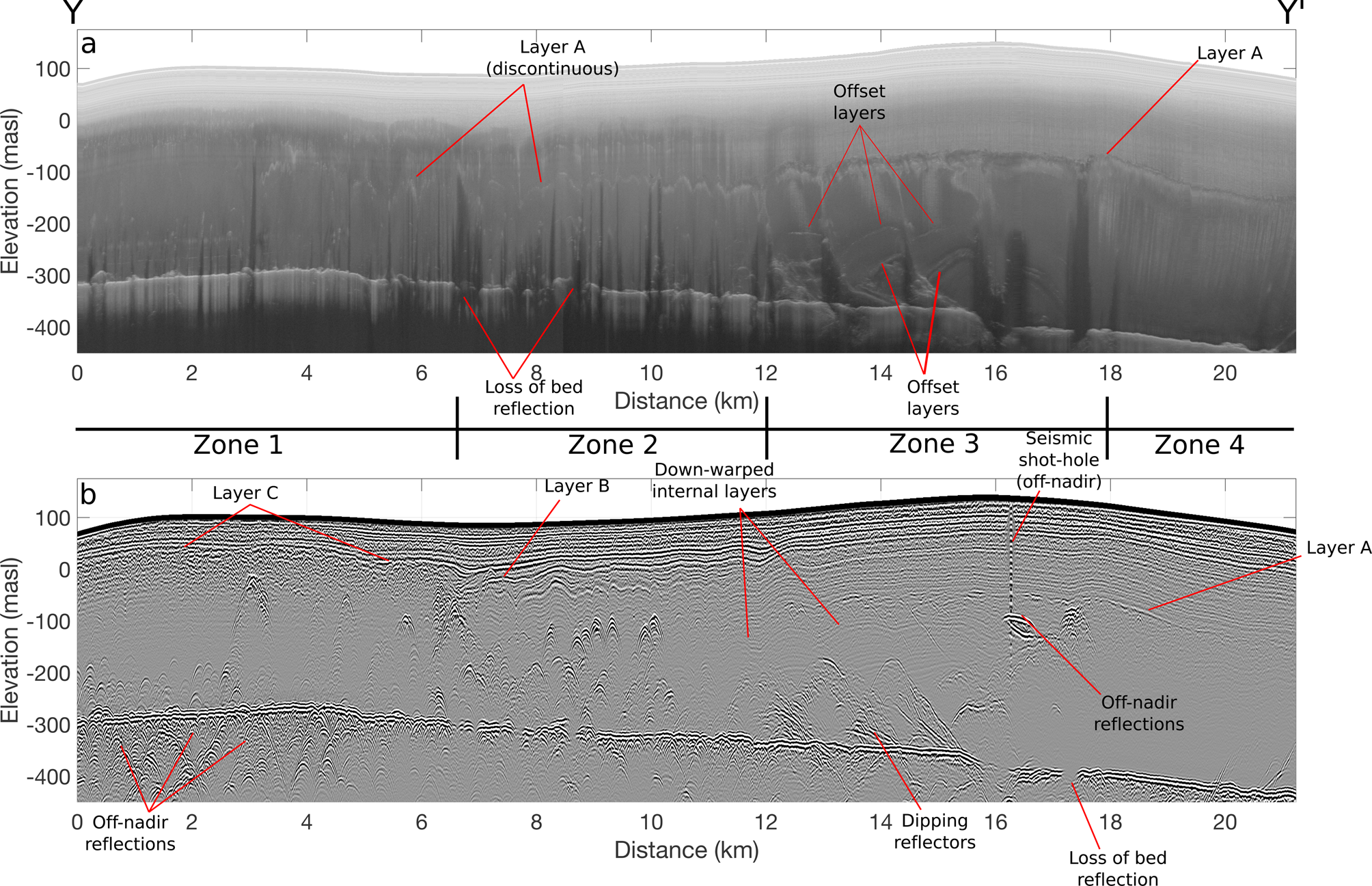
Fig. 3. Transect Y–Y’ across the ice rise using 750 MHz (a) and 7 MHz (b). Both echograms are corrected for surface topography. The near surface reflection near the divide visible in the 7 MHz data is from a seismic shot hole. Details of four distinct structural zones, labeled zones 1 through 4 are discussed in the text.
2. Data and methods
2.1 Radar systems
Two radar systems were used to map englacial structures, internal layers, and ice thickness at CIR in November and December 2015. We used the University of Washington (UW) high-frequency, mono-pulse system with resistively loaded dipole antennas operating at the center frequency of 7 MHz; range resolution is ~6 m in ice (1/4 wavelength). The transmitter and receiver were towed inline (p-polarized) behind a skidoo; the receiver was triggered by the airwave from the transmitter. The airwave causes signal saturation in the upper 0.15 μs (~25 m) of the received records. Each record consists of 1024 stacked waveforms to improve the signal-to-noise ratio. Positions and elevations of records were located using GPS with average spacing along the track of 2.7 m. Data processing includes bandpass filtering, and accounting for the distance between the transmitter and receiver (39 m). We present unmigrated data here because the diffraction hyperbolas form a central part of our analysis. At 7 MHz, internal reflections below the firn are caused primarily by contrasts in electrical conductivity (Fujita and others, Reference Fujita1999). Englacial reflections, measured as a function of radar two-way travel time, were converted to a depth below the surface using a wave speed of 168.5 m μs−1 in ice and 300 m μs−1 in air. Wave-speed in the firn was estimated by calculating the dielectric constant using an empirical depth-density model (Herron and Langway, Reference Herron and Langway1980) and Looyenga's mixing equation (Looyenga, Reference Looyenga1965).
Uncertainty in the depth to a nadir reflecting layer arises from uncertainty in the wave speed in ice (~1 m μs−1, which corresponds to 0.6% of the depth to the reflector), and from ambiguity in picking the two-way travel time (0.01 μs or ~1 m in ice); total uncertainty for a reflector at 500 m depth is ~4 m. However, mono-pulse radars have significant gain from side lobes in the radiation pattern in off-nadir directions, both fore and aft and either side of the transmitter–receiver pair (Arcone, Reference Arcone1995; Jacobel and others, Reference Jacobel, Christianson, Wood, Dallasanta and Gobel2014). A consequence is that strong returns from targets within the side lobes have arrival times greater than nadir reflections; our 7 MHz profiles on CIR often show strong reflections that appear up to 100 m below the basal reflector, which complicates interpretation.
We also used an ultra-high-frequency (UHF) pulsed chirp radar developed by the Center for the Remote Sensing of Ice Sheets (CReSIS), operating over 300 MHz of bandwidth centered at 750 MHz, with a range resolution of 43 cm in ice (Lewis, Reference Lewis2015; Lewis and others, Reference Lewis2015). A 600–900 MHz linear FM chirp is transmitted at a 50 kHz pulse repetition frequency and directly captured using a 1 giga-sample per second analogue-to-digital converter. An eight-element wideband dipole antenna array is used with a power combiner to create a directive beam pointed toward nadir (Rodriguez-Morales and others, Reference Rodriguez-Morales2014). The 1 μs pulse duration results in signal saturation in the upper ~90 m, but the UHF yields enhance sensitivity to dielectric changes deeper in the ice. Transmission power was 5 W. Surface topography and location were recorded with GPS. Data were migrated using a Fourier transform method (Leuschen and others, Reference Leuschen, Gogineni and Tammana2000) and processed using the standard CReSIS toolbox (https://ops.cresis.ku.edu/wiki/index.php/Main_Page).
The lower frequency of the UW system enables improved layer coherence and reduced radar clutter, while the CReSIS system has enhanced range resolution. The UW system is more robust for travel over rough terrain and during high winds, typical of conditions on CIR, so surveys with the CReSIS system were made at high spatial density in the vicinity of camp.
2.2. Waveform modeling
We use the open-source waveform modeling software gprMax (Warren and others, Reference Warren, Giannopoulos and Giannakis2016) to test hypotheses for the origin of the observed englacial structures observed across CIR. gprMax solves Maxwell's equations in two or three dimensions using the Finite-Difference Time Domain method. We use the default setting for absorbing boundary conditions. We model the 7 MHz waveforms in 2D with a Hertzian dipole point source and a receiver separated by 39 m. Modeling the 750 MHz waveforms is computationally impractical due to the high resolution required for the short wavelength of the UHF system, and the km2-scale model domain. Dielectric properties used in the model experiments are given in Table 1.
Table 1. Dielectric properties of the different materials used in waveform modeling

Values are from Christianson and others (Reference Christianson2016), except for brine-rich ice, which uses the dielectric properties of sea ice from Morey and others (Reference Morey, Kovacs and Cox1984).
3. Radar-detected englacial structures
Radar profiles at 750 and 7 MHz along X–X’ (Fig. 2) reveal a highly reflective and spatially continuous layer (hereafter referred to as Layer A) at both frequencies. Internal horizons are visible at depths below Layer A at 7 MHz, but only rarely at 750 MHz, likely because of the high sensitivity of UHF systems to scattering (Lewis and others, Reference Lewis2015) and steeply dipping layers (Holschuh and others, Reference Holschuh, Christianson and Anandakrishnan2014). Numerous stacks of diffraction hyperbolas extend up to 300 m above the bed, where total ice thickness is ~500 m. Internal reflection horizons between the stacks of diffraction hyperbola are often warped downwards, forming arcs with amplitudes of up to 40–50 m (Fig. 2c). Many of these diffraction hyperbolas intersect Layer A and overlie locations where the bed echo is obscured.
Radar profiles along Y–Y’ (Fig. 3) reveal four distinct zones (labeled Zones 1–4). Zone 1 crosses the lower (grid southwest) ridge of the ice rise. The deepest continuous layer in Zone 1 (at ~100 m depth, which we call Layer C) marks a transition from conformal layers to disturbed ice. We infer that Layer C represents a transition from shelf or streaming flow to divide flow at the lower ridge. Layer A is faintly visible in the 750 MHz data in part of Zone 1 where it is highly deformed and discontinuous. In contrast to other zones, Layer A does not mark the uppermost limit of diffraction hyperbolas in Zone 1; hyperbolas at ~3 km along Y–Y’ extend ~75 m above Layer A. Although the tops of the strong diffraction hyperbola in this zone extend ~275 m above the bed, the bed reflection is reduced but not completely obscured. While strong mid-depth diffraction hyperbolas are less abundant than elsewhere, hyperbolas near the bed are more numerous.
In Zone 2, Layer C is clearly visible, but does not represent the deepest undisturbed ice. A strongly reflective layer ~30 m deeper than Layer C represents the deepest undisturbed ice in Zone 2 (Fig. 3). The pattern of deformation of Layer B is similar to that of Layer A, but it is more muted and is not punctuated by numerous diffraction hyperbolas as is Layer A. This suggests that Layers A and B experienced a similar history of deformation, but Layer B was not subjected to the same process that caused the diffraction hyperbolas. Layer B terminates at a stack of diffraction hyperbolas at ~6 km along Y–Y’, which coincides with the transition where Layer A begins to be coincident with the upper limit of diffraction hyperbolas. Layer A does not appear brighter than others in the 7 MHz data in this zone, but it is clearly discernable in the 750 MHz data. Multiple stacks of diffraction hyperbolas extend up to ~250 m above the bed and often obscure the bed reflection.
In Zone 3, an off-nadir reflection from a seismic shot-hole that we drilled at the crest of the ridge is visible in the 7 MHz data. While the seismic shot-holes only reached a depth of ~40 m, this reflection appears deeper because it is off-nadir. The layers above Layer A are relatively undisturbed. Below Layer A, another strong reflection intersects with the shot-hole reflection, which is from off-nadir reflections from the same features that cause the englacial diffraction hyperbolas. The amplitude of the reflection from Layer A is larger than it is in Zone 2 and the layer is less deformed. On the grid northeast side of the ridge, a single stack of hyperbolas that intersects Layer A blocks the bed echo. Deep reflectors with an apparent dip of ~10° downwards to the bed are evident between 14 and 16 km in Zone 3. We interpret these to be the same as the features that caused the strong diffraction hyperbolas elsewhere, but they have been sheared due to ice flow since the time of grounding. These dipping reflectors do not block the bed echo. Two layers below Layer A are visibly offset in the 750 MHz data across these dipping reflectors. Directly beneath the divide of the ridge (~16 km in Y–Y’), a deep reflector subparallel to the bed overlies a region of very faint bed echo.
In contrast to other zones, Zone 4 is mostly free of diffraction hyperbolas and the bed reflection is strong. Layers A, B and C are all visible in the 7 MHz data; Layer A is visible at both 7 and 750 MHz. All three of these layers are undisturbed and conformal with layers above and below. Noteworthy features in Zone 4 are dipping reflectors that intersect with the bed and lean toward the ice shelf (20–21 km in Y–Y’). We interpret these to be basal crevasses formed slightly inland of the grounding-line of CIR.
Figure 4 shows three additional profiles surveyed parallel to Y–Y’ at 750 MHz. These show more frequent loss of bed echo and substantial deformation of internal layers in the central plain of the ice rise compared to the grid northeast flank of the main ridge. Obscured bed reflection beneath the diffraction hyperbolas and steeply dipping deep reflectors is a characteristic feature in Zone 3. A linear feature visible in the 125 m resolution MODIS imagery (Haran and others, Reference Haran, Bohlander, Scambos, Painter and Fahnestock2014) intersects the modern grounding line near the rifted zone in the ice shelf downstream of the ice rise, and trends parallel with the main ridge crest (shown in Figs 1 and 4). The lineation marks a break in slope in the Reference Elevation Map of Antarctica (REMA) DEM (Howat and others, Reference Howat, Porter, Smith, Noh and Morin2019) and also marks (i) the onset of high-frequency deformation and a general deepening trend of Layer A to the grid southwest, and (ii) the boundary of dipping reflectors that intersect the bed and divide the offset layers shown in Figure 4a. Upstream (grid northeast) of the surface lineation in Figure 4d is the largest region of lost bed reflection, where the bed echo is lost for a length of ~1.5 km.
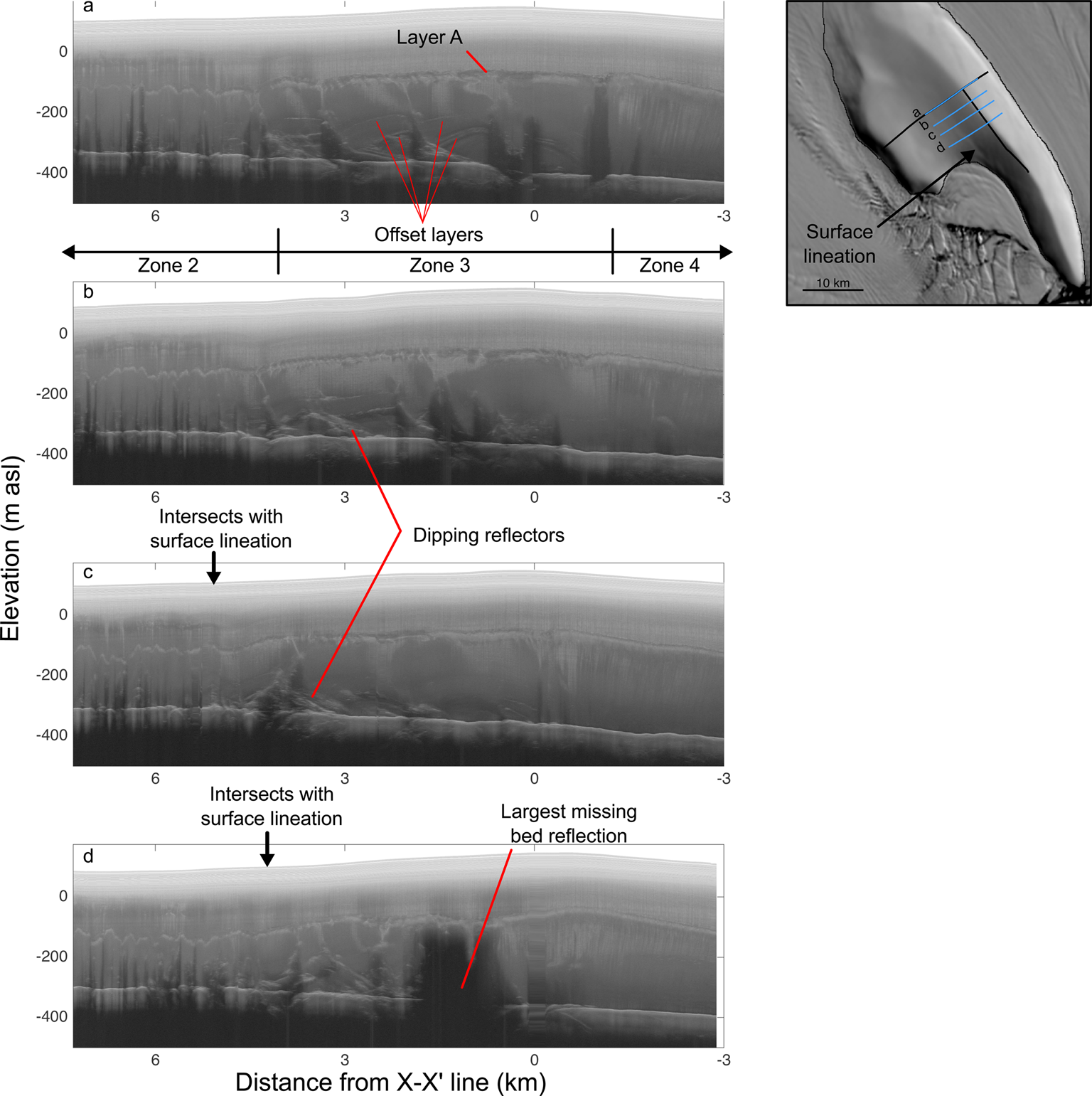
Fig. 4. The 750 MHz radar profiles across the main ridge of the ice rise, showing the distribution of basal reflectors and the loss of bed reflection on the inner flank of the ice rise. Top to bottom profiles correspond to top to bottom tracks on the map. Distance on horizontal axis is relative to the X–X’ profile, shown in black on the map, with negative distances corresponding to the shelf-proximal (grid northeast) side of the main ridge. Panel (a) shows a sub-section of Y-Y’ (Fig. 3). Profiles in panels (c) and (d) intersect a visible surface lineation marked on the map; intersection locations are denoted by black arrows on each profile.
4. Interpretation of radar-detected Layers A, B and C
Layers A, B and C each mark the transition from undisturbed, conformable layering to disturbed ice containing numerous diffraction hyperbolas over different sections of CIR (Figs 3, 4). We interpret the ice above these layers to be derived from local accumulation, while the disturbed ice below was formerly floating or fast flowing. This is consistent with the observations of similar reflection horizons within the modern Ross Ice Shelf (Tinto and others, Reference Tinto2019; Das and others, Reference Das2020) and the Brunt Ice Shelf (King and others, Reference King, Rydt and Gudmundsson2018). We interpret each of these layers to represent separate grounding or basal-freezing events: Layer A represents the grounding of the main (grid northeast) ridge of the ice rise; Layer B represents the grounding or stagnation of fast flow in the central plain; and Layer C represents the final grounding event at the shallower (grid southwest) ridge. These events are depicted schematically in Figure 5. This supports the sequence of events outlined by Bindschadler and others (Reference Bindschadler, Roberts and Iken1990), but also adds a separate event in which the central area of the ice rise grounded or stagnated after the main ridge, but before the shallow ridge. It is likely that these radar data hold clues to more stages of evolution that we have not identified.

Fig. 5. Interpretation of Layers A, B and C in terms of the evolution of Crary Ice Rise. Arrows represent schematic flow patterns. Note that there are likely intermediate stages that are not captured by our analysis.
The depth of Layer A increases across the surface lineation visible in the MODIS imagery (Haran and others, Reference Haran, Bohlander, Scambos, Painter and Fahnestock2014) (Fig. 4). Several kilometers downslope (grid southwest) of the lineation, it becomes highly deformed with the amplitudes of ~60 m over short distances. The deepening and increased deformation of Layer A with respect to the surface lineation is consistent with the hypothesis that the surface lineation delineates a former grounding line. The stratigraphic sequence is similar to that observed in the flat-ice terrain between Engelhardt Ice Ridge and Kamb Ice Stream, which has been interpreted to be a relict grounding line (Catania and others, Reference Catania, Conway, Raymond and Scambos2006).
5. Origin of diffraction hyperbolas and waveform model results
Stacks of diffraction hyperbolas are prominent and ubiquitous internal structures in the central section of CIR. The bed reflections beneath the largest stacks are often 30–50 dB weaker than nearby reflections that are not beneath the hyperbolas (Fig. 6). Such strong attenuation of bed reflections is not normally found within grounded ice, but since CIR likely formed from re-grounding of the Ross Ice Shelf (Bindschadler and others, Reference Bindschadler, Roberts and Iken1990), it is likely that these features are due to processes within the former ice shelf. Two processes within ice shelves have been demonstrated to attenuate radar waves: marine ice accretion and lateral brine infiltration. Marine ice has been observed in present-day rifts and crevasses around Antarctica (Khazendar and Jenkins, Reference Khazendar and Jenkins2003; Jansen and others, Reference Jansen, Luckman, Kulessa, Holland and King2013; Kulessa and others, Reference Kulessa, Jansen, Luckman, King and Sammonds2014; Arcone and others, Reference Arcone2016), and its occurrence often obscures radio echoes from the bases of ice shelves. Concentrated brine pockets caused by lateral infiltration of seawater from rifts along firn/ice horizons are observed in the McMurdo Ice Shelf today (Morse and Waddington, Reference Morse and Waddington1994; Grima and others, Reference Grima2016; Campbell and others, Reference Campbell, Courville, Sinclair and Wilner2017). While the presence of either brine layers or marine ice would suggest past rifting of the ice that now forms CIR, establishing the englacial composition is important for evaluating the evolution of the ice rise and the ice shelf. For example, brine layers change the temperature, density and chemistry of the firn, but have little impact on the dynamics of the ice shelf (Thomas, Reference Thomas1975). In contrast, large deposits of soft marine ice inhibit fracture propagation, allow increased internal deformation and strengthen the ice shelf (e.g. Khazendar and others, Reference Khazendar, Tison, Stenni, Dini and Bondesan2001; Kulessa and others, Reference Kulessa, Jansen, Luckman, King and Sammonds2014, Reference Kulessa2019), and thus could have played an important role in the formation of CIR.
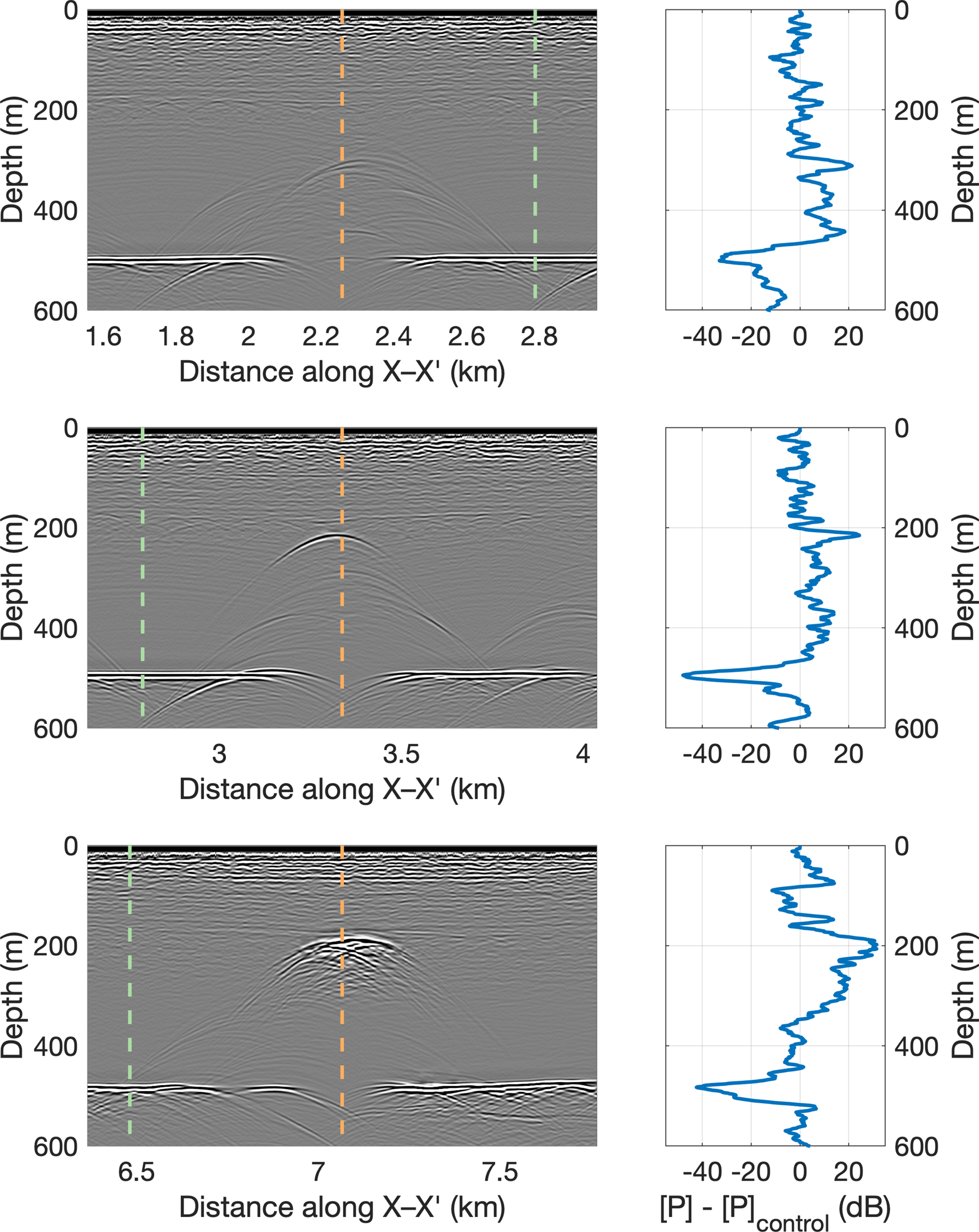
Fig. 6. Return power from 7 MHz radar measurements along profile X–X’. The blue curves in the right-hand column are calculated by averaging return power horizontally on a 25 m-wide transect centered on the orange line in the left-hand column and subtracting off the same average around the green line. Curves represent a running average using a window of 10 vertical meters. Return power is calculated using the definition of Gades and others (Reference Gades, Raymond, Conway and Jacobel2000).
We use the gprMax waveform model (Warren and others, Reference Warren, Giannopoulos and Giannakis2016) to test these hypotheses: radar attenuation is caused by accreted marine ice in former basal crevasses and/or rifts (H1); and radar attenuation is caused by pockets of brine trapped within the ice at the former firn-ice transition (H2). Studies of brine infiltration layers have been conducted in areas where brine is actively entering an ice shelf (e.g. Grima and others, Reference Grima2016; Campbell and others, Reference Campbell, Courville, Sinclair and Wilner2017), or recharging from groundwater into englacial systems (Badgeley and others, Reference Badgeley2017), but we are not aware of studies that have detected ancient brine pockets that are frozen and disconnected from the source, which could have very different dielectric properties from actively percolating liquid brine. Thus, we assume an effective dielectric constant of 4.1, calculated using Looyenga's mixing formula (Looyenga, Reference Looyenga1965) for ice with 4.5% seawater inclusions by volume, which is a maximum estimate for brine concentration in a flooded firn layer (Thomas, Reference Thomas1975). This dielectric constant is similar to that of sea ice containing brine inclusions (Morey and others, Reference Morey, Kovacs and Cox1984). The conductivity of the brine layer is much more difficult to estimate because it depends both on whether the brine is at the percolation threshold (Lux, Reference Lux1993) (i.e. if an electrical pathway connects all parts of the brine pocket), and on the chemistry of the brine. Thus, we assume the conductivity of the layer is also similar to that of sea ice with brine inclusions, which ranges from ~0.01 to 0.1 S m−1 (Morey and others, Reference Morey, Kovacs and Cox1984).
Due to the large number of unknowns and the wide range of possible geometries, we take an ensemble approach to modeling the radar signatures of the englacial structures in order to understand how bed echoes may be attenuated or lost completely. Our ensemble consists of 28 members and one control simulation with no brine layer and no marine ice layer. We model vertical brine layer thicknesses of 1 and 10 m, which we assume to be a reasonable range based on observations of active brine layers (Campbell and others, Reference Campbell, Courville, Sinclair and Wilner2017). We use brine layer conductivities of 0.1 and 0.01 S m−1, in order to span the range of sea-ice conductivities (Morey and others, Reference Morey, Kovacs and Cox1984). Modeled horizontal layer widths are 10, 50, 100 and 200 m (for both brine and marine ice), to match observed loss of bed echo. We use vertical marine ice thicknesses of 10, 150 and 305 m to span the possible range from a deposit at the top of a fracture to complete filling of the fracture. In all runs, the top of the brine or marine ice layer lies 305 m above the bed (150 m below the surface). Total ice thickness (including a 24 m firn column) is 455 m in all runs, which is an intermediate value for ice thicknesses at CIR. The ice-sheet bed is treated as a 10 m-thick layer of frozen till overlying unfrozen bedrock, based on observations of till clasts frozen to the drill during hot water drilling in the 1980s (Bindschadler and others, Reference Bindschadler, Roberts and Iken1990). The model domain is 1200 m wide by 600 m tall and is sampled by 119 different transmitter–receiver (39 m separation) positions at intervals of 10 m. Horizontal and vertical model resolution is 0.8 m. Model geometry is shown in Figure 7. Dielectric properties of the modeled materials are given in Table 1.

Fig. 7. Schematic of gprMax model geometry. Layer thickness, layer width and layer type (i.e. marine ice or brine) are variable model parameters. Here we show the model configuration for marine ice with width = 100 m and thickness = 150 m. For the rift configuration, the layer reaches the bedrock (thickness = 305 m); for the brine configuration, the layer is one to two orders of magnitude thinner than shown here. The top of the layer is always at the depth shown here. Transmitter and receiver are stepped across the domain from left to right at 10 m intervals. All domain boundaries are treated as perfect absorbers of transmitted energy.
Results of the model ensemble show that reflector composition (i.e. brine or marine ice), width and thickness all exert strong controls on the strength of the bed echo from the base of the ice rise. To calculate the return power attenuated by the brine or marine ice layer in each run, we averaged the bed return power beneath the layer over 50 m horizontally and 10 m vertically and subtracted off the average over the same area in the control run. These results are shown in Figure 8a. For a given layer width, the thickest marine ice layer (305 m) is always the strongest attenuator, followed by the 150 m-thick marine ice layer. The 10 m-thick marine ice layer is always the weakest attenuator. The relationship between layer properties and attenuation is less straightforward for the brine layers. For the 10 m-thick brine layer, the two conductivity values result in similar attenuation values for layers 10–100 m wide, while the lower conductivity value results in stronger attenuation for 200 m wide layer. Layer thickness has a relatively small effect on bed return power attenuation for the more conductive brine layer, but a large effect for the less conductive brine layer. We find 11 cases that result in strong enough attenuation to explain the >30 dB decrease in bed echo beneath diffraction hyperbolas in our radar data. This shows that the degree to which the bed echo is attenuated cannot be used to definitely determine whether the diffraction hyperbolas are caused by marine ice or brine layers.
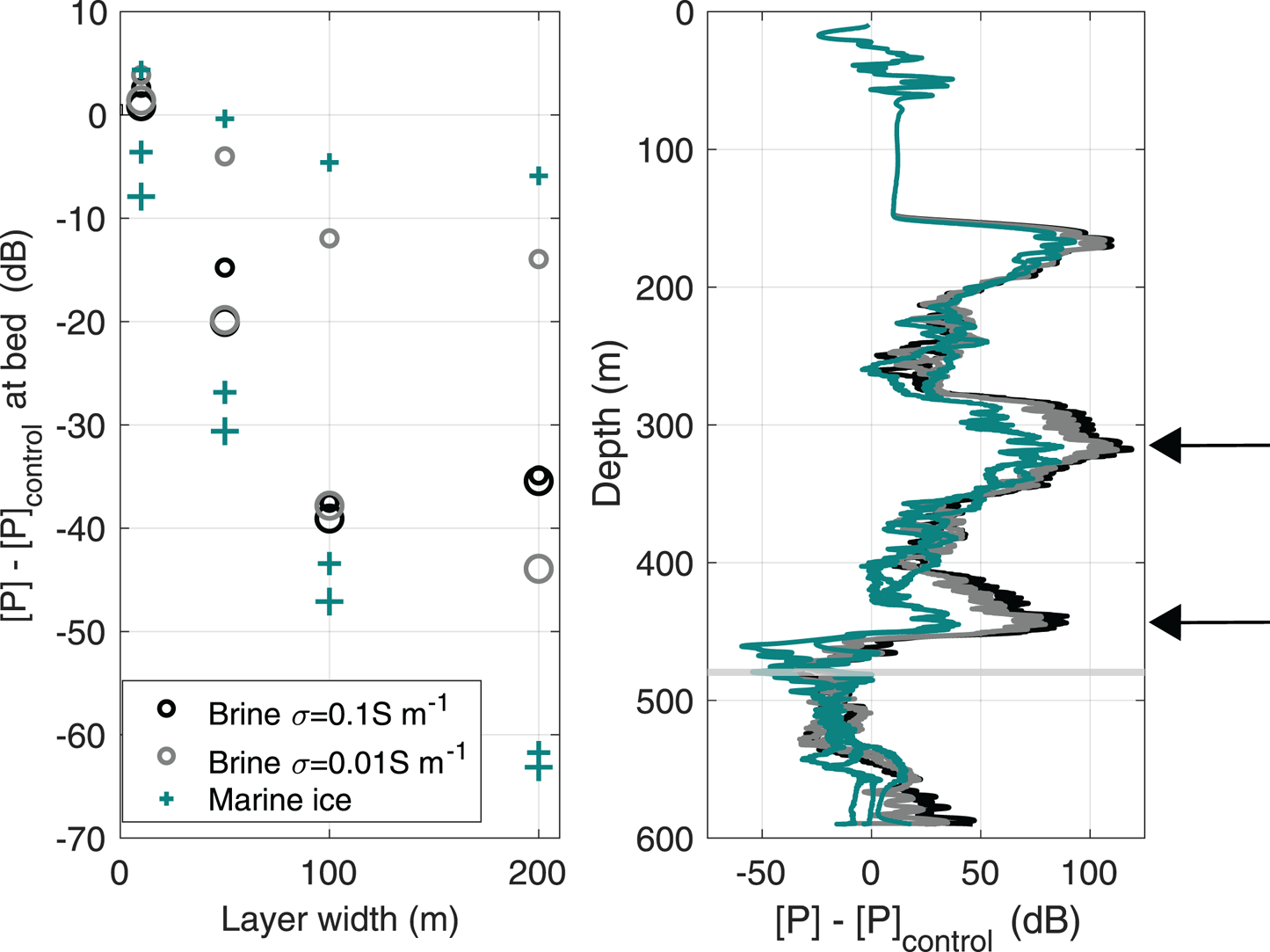
Fig. 8. (a) Results of the return power at the bed for each member of gprMax model ensemble, minus the control run. Return power values are averaged over 10 vertical meters and 50 horizontal meters at the bed in the center of the domain. We consider values ≤−30 dB to be consistent with our observations. Marker size corresponds to layer thickness: For marine ice, small = 10 m; medium = 150 m; large = 305 m. For brine layer, small = 1 m; large = 10 m. (b) Return power minus control run for ensemble members with width = 100 m as a function of depth. Power is averaged over 50 horizontal meters spanning the domain center and smoothed using a 10 m running average. Reflection multiples are indicated by black arrows. Horizontal grey bar indicates the location of the ice rise bed. Colors are the same as those in panel (a). Different layer thicknesses are not denoted because material properties have the strongest control on the results. Results of the full ensemble are shown in the Appendix (Fig. 10).
Next, we examine return power as a function of depth to determine if the model can help distinguish between the cases that could explain the observed loss of bed echo. Figure 8b shows the average return power (minus the control) over the 50 horizontal meters spanning the domain center as a function of depth for selected members of the ensemble; the full ensemble results are shown in Figure 10 in Appendix. We find two strong reflection multiples beneath the brine layers in all scenarios. A single strong reflection multiple is also apparent beneath the marine-ice layer, but is 20–30 dB weaker than for brine layers of the same width. Our data do not show reflection multiples beneath the layers obscuring bed echoes, so we rule out the hypothesis that the bed echoes are obscured by brine layers. A rough or diffuse interface between the meteoric ice and marine ice would further decrease the strength of the multiple without significantly decreasing the attenuation. Such a rough and diffuse transition could result from the mélange of sea ice, icebergs, snow, and marine ice that often fill the tops of rifts (Fig. 9) (Rignot and MacAyeal, Reference Rignot and MacAyeal1998; King and others, Reference King, Rydt and Gudmundsson2018). For a given width of modeled marine ice deposit, there is only a 2–5 dB difference in bed return power attenuation between layers 150 m thick and 305 m thick (Fig. 8a); therefore, a layer 305 m thick that transitions gradually from locally accumulated glacier ice to marine ice over tens of meters would be almost as effective at obscuring the bed echo as the uniform 305 m-thick layer we have modeled here, but the reflection at the upper boundary would be greatly diminished. A gradual transition would also explain the stacks of diffraction hyperbolas we observe in the radar data by providing many smaller dielectric contrasts that would each cause a reflection. A smooth transition over 1–10 m would have little effect on the reflectivity of the brine layer because these layer thicknesses are already very close to (or below) the 6 m range resolution of a 7 MHz system. Therefore, we interpret the observations of diffraction hyperbolas overlying a loss of bed echo to be most consistent with the presence of marine ice deposits hundreds of meters thick and up to (and perhaps exceeding) 1.5 km wide (e.g. Fig. 4d). While this is a large amount of marine ice, it is reasonable by comparison with the thick packages of marine ice accreted within and beneath modern ice shelves. Bands of marine ice hundreds of meters thick and continuous for up to hundreds of kilometers in extent have been detected at the base of ice shelves (Thyssen and others, Reference Thyssen, Bombosch and Sandhäger1993; Fricker and others, Reference Fricker, Popov, Allison and Young2001) and within suture zones (e.g. Craven and others, Reference Craven, Allison, Fricker and Warner2009; Jansen and others, Reference Jansen, Luckman, Kulessa, Holland and King2013).
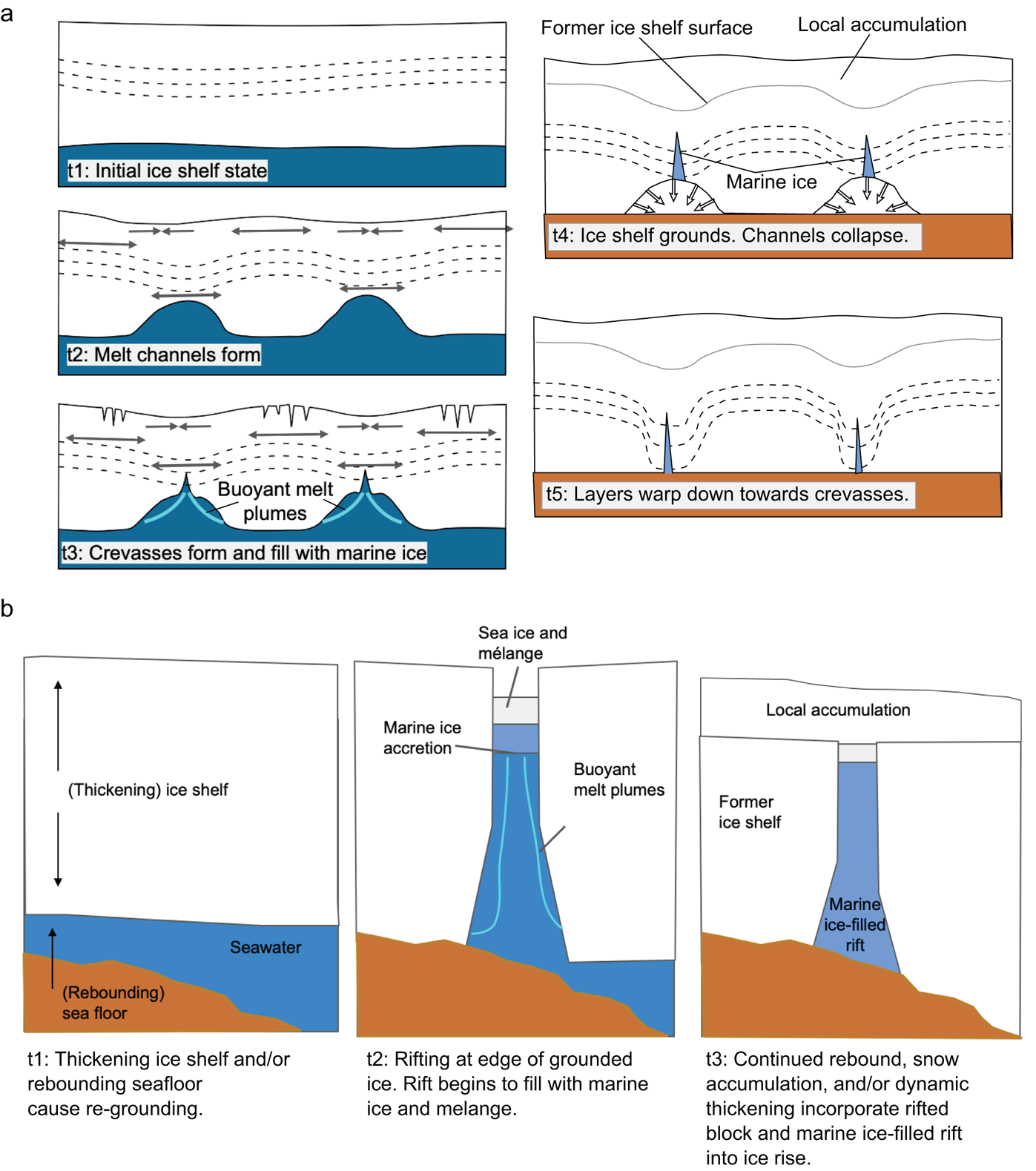
Fig. 9. Interpretation of processes that could cause the structures observed in our radar surveys. (a) Basal melt channels in an ice shelf causing flexure and crevassing (modified from Vaughan and others, Reference Vaughan2012). Black arrows show direction and relative magnitudes of deviatoric stresses. Crevasses fill with marine ice and collapse of basal melt channels after grounding causes down-warping of internal layers toward filled crevasses, such as those seen in Figure 2c. (b) Ice shelf rift filling with marine ice (modified from Khazendar and Jenkins, Reference Khazendar and Jenkins2003) and being incorporated into grounded ice.
6. Discussion
Figure 9 illustrates possible processes that could cause the marine ice structures observed in our radar surveys and modeled above. Three observations distinguish between former basal crevasses and former rifts in our data:
(1) Features that we determine to be former rifts coincide with Layers A and B, which we take to mark the transitions from shelf and/or streaming ice to locally accumulated ice (see Section 4). Basal crevasses are detected below these layers and did not penetrate the full ice thickness. The tops of rifts fill with snow, sea ice and icebergs, while marine ice accretion within rifts occurs from the top downwards as melting of the rift walls drives convection (Khazendar and Jenkins, Reference Khazendar and Jenkins2003). The freezing-point dependence on pressure causes buoyant plumes of supercooled meltwater to refreeze at shallower depths within crevasses and rifts (Lewis and Perkin, Reference Lewis and Perkin1986).
(2) The features we identify as marine ice-filled rifts do not exhibit down-warping of internal layers toward the stacks of hyperbolas, while those identified as basal crevasses are often flanked by down-warping internal reflectors on either side (Fig. 2c). Basal crevasses often form at the apexes of basal melt channels (Vaughan and others, Reference Vaughan2012), and these channels would have collapsed after the ice shelf grounded and the ice rise thickness exceeding hydrostatic equilibrium, causing down-warping of internal layers (Fig. 9). We note that if rifts are not filled completely with marine ice, the collapse of the unfilled bottom of the rift after grounding would cause similar down-warping of internal layers. However, we do not observe down-warping of layers toward features that intersect Layer A, so we do not believe this is common at CIR. This is consistent with the complete infilling of rifts with marine ice on the modern Larsen C ice shelf (Jansen and others, Reference Jansen, Luckman, Kulessa, Holland and King2013; Kulessa and others, Reference Kulessa, Jansen, Luckman, King and Sammonds2014).
(3) Rifts are more laterally extensive than basal crevasses, and are thus associated with more extensive loss of the bed echo (e.g. Fig. 4d).
The offset layers labeled in Zone 3 in Figures 3, 4a support the interpretation that the largest regions of lost bed echo are caused by former rifts in the ice shelf. Two sets of internal reflecting horizons at ~−200 and −300 m elevation are clearly offset between these blocks, as from differential motion across a fault. We interpret these faults to be former rifts in the ice shelf, as we also find above areas of missing bed reflection (e.g. at −1 km in Fig. 4a). The apparent dip of these offset layers suggests deformation due to vertical shear. Although there is no detectable offset in Layer A across these faults, the deeper layers are significantly offset. Therefore, the differential motion that caused the offset of these layers must have occurred before the establishment of Layer A. This could be due to irregular melting of the base and/or sides of the rifted blocks while they were still part of the ice shelf. We interpret the continuity of Layer A across the top of these blocks to indicate that they were incorporated into the grounded part of the ice rise over a relatively short span of time, and possibly at the same time.
Our radar surveys reveal that CIR contains abundant marine ice, which likely accreted within rifts and basal crevasses in the Ross Ice Shelf shortly after it re-grounded at this site. Similar complex basal structures beneath the Ross Ice Shelf have been detected by radar (Jezek and others, Reference Jezek, Bentley and Clough1979; Jezek and Bentley, Reference Jezek and Bentley1983). It is possible that marine ice deposits within slow-flowing grounded ice may be common in West Antarctica due to the late Holocene re-advance of the grounding line to its current configuration (Kingslake and others, Reference Kingslake2018). Matsuoka and others (Reference Matsuoka, Gades, Conway, Catania and Raymond2009) identified a feature they interpreted to be caused by accreted marine ice in crevasses near a former grounding line of Kamb Ice Stream; radar-detected basal crevasses near that feature (Catania and others, Reference Catania, Conway, Raymond and Scambos2006) may also contain marine ice. It is possible that marine ice exists within relict basal crevasses identified at other locations around Antarctica, such as the Henry Ice Rise (Kingslake and others, Reference Kingslake2018; Wearing and Kingslake, Reference Wearing and Kingslake2019). Basal crevasses in slow-moving grounded ice creep shut quickly (van der Veen, Reference van der Veen1998); unless some material other than glacier ice fills the crevasses to create a dielectric contrast, it is unlikely they could be detected by radar after closing. The tilting of the crevasses within Henry Ice Rise (Kingslake and others, Reference Kingslake2018; Wearing and Kingslake, Reference Wearing and Kingslake2019) especially indicates that these are not currently open basal crevasses because the shear deformation that tilted them would also have acted to close them (van der Veen, Reference van der Veen1998). Whether or not they are filled with enough marine ice (or another material) to be important to ice dynamics is unclear.
Thick layers of marine ice accrete at the bottom of ice shelves and within suture zones, with maximum estimated thicknesses of up to 350 m (Thyssen and others, Reference Thyssen, Bombosch and Sandhäger1993; Grosfeld and others, Reference Grosfeld, Jacobs and Weiss1998; Fricker and others, Reference Fricker, Popov, Allison and Young2001). However, accreted marine ice is <10 m thick at the base of the modern Ross Ice Shelf (Neal, Reference Neal1979; Zotikov and others, Reference Zotikov, Zagorodnov and Raikovsky1980), and we do not detect a continuous basal layer in our data. We thus attribute the formation of marine ice at CIR to localized processes such as refreezing of buoyant melt plumes in rifts and basal crevasses (Fig. 9) (Khazendar and Jenkins, Reference Khazendar and Jenkins2003), rather than to large-scale oceanographic conditions extensive beneath the whole Ross Ice Shelf. Marine ice deposits in former basal crevasses have been documented in icebergs calved from the Amery Ice Shelf in East Antarctica (Warren and others, Reference Warren1993, Reference Warren, Roesler, Brandt and Curran2019). The marine ice in these icebergs was found to be rich in organic matter and iron, indicating active biology beneath the ice shelf. It is possible that the marine ice within CIR contains an archive of biological conditions beneath the Ross Ice Shelf more than a millennium ago.
The marine ice within CIR may have played a significant part in its evolution by healing ruptures formed during the grounding events, thereby strengthening and consolidating the floating ice shelf (Rignot and MacAyeal, Reference Rignot and MacAyeal1998) and dynamically coupling it to the grounded ice rise. Such strengthening has been documented at the Filchner-Ronne, Brunt/Stancolm-Wills and Larsen C ice shelves (Rignot and MacAyeal, Reference Rignot and MacAyeal1998; Holland and others, Reference Holland, Corr, Vaughan, Jenkins and Skvarca2009; Khazendar and others, Reference Khazendar, Rignot and Larour2009; Jansen and others, Reference Jansen, Luckman, Kulessa, Holland and King2013); marine ice in rifts may have played a role in preventing Larsen C from disintegrating in the same fashion as Larsen B (Kulessa and others, Reference Kulessa, Jansen, Luckman, King and Sammonds2014). In the Brunt Ice Shelf, an ice mélange consisting partially of marine ice binds together rift-bounded blocks of glacier ice, making the ice shelf effectively a series of icebergs and ice tongues that have been sutured together (King and others, Reference King, Rydt and Gudmundsson2018). The same may have been true locally during the formation of CIR, where marine ice accretion could have connected the grounded ice rise with the ice shelf across shear and rift zones, increasing the dynamical coupling of the ice rise to the Ross Ice Shelf and increasing its buttressing effect on the grounded ice-sheet upstream. Marine ice within fractures may also have inhibited rift propagation, thereby supporting the integrity of the ice shelf (Jansen and others, Reference Jansen, Luckman, Kulessa, Holland and King2013; Larour and others, Reference Larour, Rignot and Aubry2004; Kulessa and others, Reference Kulessa, Jansen, Luckman, King and Sammonds2014, Reference Kulessa2019). We cannot state definitively whether the rifts existed in the ice shelf before the grounding of CIR, but the rifted zone at the downstream CIR (Fig. 1b) indicates that they likely formed around the ice rise during the initial grounding event. Thus, our observations show that ice rises are able to incorporate heavily fractured and disconnected portions of the surrounding ice shelf into the grounded ice as they grow, and that marine ice formation within those fractures is likely an important part of that process.
Kamb, Mercer and Whillans Ice Streams experienced significant changes in velocity over the past millennium (Catania and others, Reference Catania, Hulbe, Conway, Scambos and Raymond2012). It is possible that there was a causal relationship between these changes and the grounding/freeze-on events that our data reveal occurred at CIR. The complex evolution of CIR is broadly consistent with the century-scale changes in ice flux upstream. The ages of the grounding events at ~1100 and ~580 yr BP derived from borehole thermometry (Bindschadler and others, Reference Bindschadler, Roberts and Iken1990) would likely be affected by the presence of the large marine ice deposits we reveal here, which could have created a very different initial temperature state than assumed in their model. Thus, the timing of these events may have been similar to the timing of the stagnation and reactivation of Whillans Ice Stream ~860 and ~450 yr BP, respectively. The stagnation of Kamb Ice Stream ~200 yr BP is also roughly coincident with Bindschadler and others’ (Reference Bindschadler, Roberts and Iken1990) estimate of the final freeze-on of the shallow ridge at CIR 130 yr BP. However, relationships between the timing of grounding and ice-stream activity remain speculative.
7. Conclusions
We mapped englacial structures within CIR using two radar systems operating at 7 and 750 MHz center frequencies. Three bright reflective horizons (Layers A, B, C) are concomitant with the tops of the strongest diffraction hyperbolas and the shallowest undisturbed locally accumulated ice. We interpret these horizons to delineate three distinct dynamic events that suggest the evolution of the ice rise was more complex than has been documented to-date. Waveform modeling and geometric arguments suggest that the diffraction hyperbolas that are ubiquitous in the central region of the ice rise are caused by marine ice deposits within former rifts and basal crevasses. The former grounding line of CIR – now incorporated into grounded ice – may still be visible as a surface lineation in MODIS imagery (Haran and others, Reference Haran, Bohlander, Scambos, Painter and Fahnestock2014).
Our surveys confirm that CIR is not a remnant of the expanded ice sheet of the last glacial period, but rather formed when the Ross Ice Shelf re-grounded locally. The lower one-half to two-thirds of the ice column consists of former Ross Ice Shelf ice, while the rest has formed from local accumulation. This is consistent with histories inferred by Bindschadler and others (Reference Bindschadler, Roberts and Iken1990), Bindschadler (Reference Bindschadler1993), Fahnestock and others (Reference Fahnestock, Scambos, Bindschadler and Kvaran2000), and Hulbe and Fahnestock (Reference Hulbe and Fahnestock2004, Reference Hulbe and Fahnestock2007) but represents the first confirmation using local geophysical measurements since the borehole thermometry of Bindschadler and others (Reference Bindschadler, Roberts and Iken1990). Marine ice accretion likely acted to reduce further ice fracturing, and to increase dynamic coupling between the grounded ice and the surrounding ice shelf (Khazendar and others, Reference Khazendar, Rignot and Larour2009), thereby enhancing its buttressing of Whillans, Mercer and Kamb Ice Streams.
Acknowledgements
This work was supported by NSF grant 1443356 to H.C. and M.K., and grant 1443552 to J.P.W. We thank Maurice Conway and Jade Cooley for assistance in the field. We also thank Antarctic Support Contract, the Air National Guard and Ken Borek Air for logistical support. The Polar Geospatial Center provided high-resolution images for planning our fieldwork. The 750 MHz UHF radar system was provided by CReSIS; we also acknowledge the use of their software, which was generated with support from the State of Kansas, NASA grant NNX16AH54 G and NSF grant ACI-1443054. UNAVCO provided GPS equipment and support. We thank Nick Holschuh, Knut Christianson, John Stone, Ed Waddington, Joseph MacGregor, Jonathan Kingslake and Martin Wearing for fruitful discussions, and Richard Hindmarsh for motivating and guiding aspects of this study. We also thank Bernd Kulessa, Frank Pattyn and two anonymous reviewers for insights and suggestions that greatly improved this manuscript. UW 7 MHz and CReSIS 750 MHz radar data and metadata are available at US Antarctic Program Data Center page: http://www.usap-dc.org/view/project/p0010026.
Appendix
Complete ensemble results
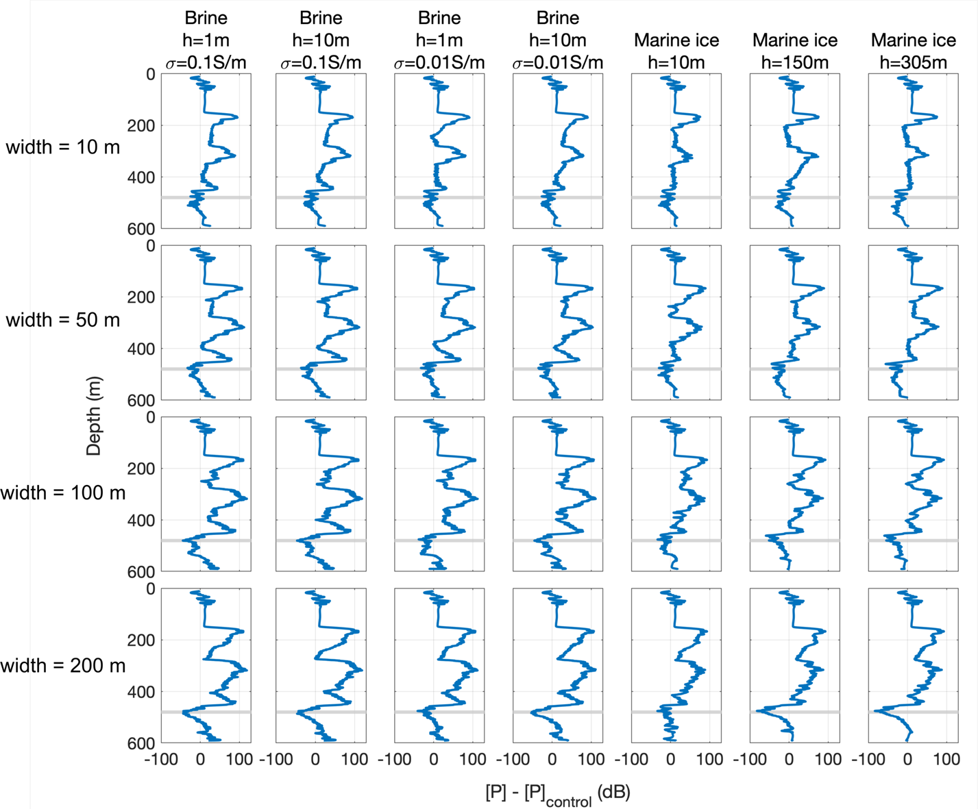
Fig. 10. Return power relative to control run for each member of the ensemble as a function of depth. Power is averaged over 50 horizontal meters spanning the domain center, and smoothed using a 10 m running average. The two very strong reflection multiples below the modeled brine layers are not observed in our data, and we thus attribute observed features to marine ice deposits. Horizontal grey bar indicates the location of the ice rise bed.


 Open access