Introduction

Thermocouples are commonly used to record changes in temperature with time. This is especially true when measurements are made at remote sites with power limitations or when large arrays of temperature sensors are deployed. Temperature measurements in snowpacks are commonly made in conjunction with snow process studies (e.g. Reference Andreas, Jordan and MakshtasAndreas and others, 2004), to determine heat flux (e.g. Reference Sturm, Perovich and HolmgrenSturm and others, 2002) or to infer the physical properties such as thermal conductivity and diffusivity of the snowpack (e.g. Reference SchwerdtfegerSchwerdtfeger, 1963; Reference Li and ZwallyLi and Zwally, 2002). Such studies require accurate and precise temperature measurements (Reference Zhang and OsterkampZhang and Osterkamp, 1995).

While investigating temperature profiles in polar firn, we noticed simultaneous temperature variations (STVs) of ~0.8°C at depths greater than 0.25 m that were correlated or anticorrelated with the thermistor reference temperature measured in the box housing the data logger. The temperature profile is shown in Figure 1, with the STVs explicitly shown in Figure 1b–d. The STVs did not decrease with depth into the snowpack as expected, nor was there the phase shift that would be expected for a temperature wave propagating into the firn. Subsequently we have found that similar, but usually smaller, STVs exist in other datasets. Because the STVs occur at multiple depths, we argue here that they are caused by an uncorrected voltage introduced within the data-logger enclosure.

Fig. 1. (a) Measured thermocouple data from the surface (gray dots), 0.5 m depth (gray curve with black squares), 1.0 m depth (black curve with black circles), 1.5 m depth (gray curve with black diamonds) and the reference temperature (black dots) within the unperturbed snowpack in Summit, Greenland, between 20 March and 30 April 2004. The daily variations decrease with depth to ~0.25 m depth and show little change at depths greater than 0.25 m. The deep temperature variations are sometimes anticorrelated (b) and at other times correlated (d) with the surface temperature. Daily changes at 1.5 m can reach 3.8°C (c). (b) and (c) have the same temperature scales on the vertical axis.

A thermocouple is a thermoelectric circuit made up of two dissimilar wires joined at one end. The temperature-dependent voltage, called the Seebeck effect, exists across the thermocouple wire junction where two compositionally dissimilar wires are joined. In practice, there are two locations where two dissimilar metals are joined. As shown in Figure 2, one is where the two dissimilar metals are soldered together to make the thermocouple (J₁ in Fig. 2), and the other is where the constantan wire is connected to a copper junction at the data logger (J₂ in Fig. 2). For the thermocouple to be useful in measuring temperature, it must depend only on the temperature at J₁. The voltage shift at J ₂ must be known, and subtracted. This is done by measuring the temperature at J₂ with a thermistor, and predicting the thermocouple effect at junction J₂ using polynomial equations published by the US National Institute of Science and Technology (NIST) (Reference Burns, Scroger, Strouse, Croarkin and GuthrieBurns and others, 1993). We refer to temperatures measured by the thermistor in the data-logger box as reference temperatures.

Fig. 2. Schematic of data logger and thermocouples. J₁–J₃ indicate wire junctions where Seebeck-effect voltage offsets occur.

The purpose of this paper is to investigate the origin of the observed STVs in thermocouple measurements and present a method for correcting STVs associated with the electronics or reference thermistor of data loggers. We show that it is very unlikely STVs are related to physical processes in the firn, and we show how they can be eliminated using temperature measurements deeper in the firn. At any time, a single voltage correction can eliminate the STVs in all the thermocouples in the array. In some cases, this correction correlates with the reference temperature, but in other cases the correction for the same reference temperature is different depending on when the temperature was recorded. Regardless of the source of the error or its dependence on the reference temperature, it is possible to correct the data, and confidence in the correction is provided by the fact that it can be shown to be appropriate for all thermocouples in the array.

The Temperature Data

Four datasets are analyzed in this paper. (1) We discuss in detail analysis of a temperature dataset we collected from a near-surface thermocouple array deployed between 20 March and 30 April 2004 at Summit, Greenland (elevation 3200 m). (2) We present more briefly an analysis of a dataset collected by others at Siple Dome (elevation 615 m), Antarctica, in 1998 (Albert, http://www.nsidc.org/data/nsidc-0100.html). (3) We analyze laboratory experiments conducted in a University of Chicago cold room to investigate STVs under laboratory conditions. (4) Examination of raw data from the Greenland Climate Network automatic weather station (AWS) at Summit, Greenland, (Reference Steffen, Box and AbdalatiSteffen and others, 1996) shows STVs, but their magnitude is much smaller than those found in the data we collected. The magnitude of the STVs appears to depend on datalogger installation methods. We refer to the weather-station data as the Summit AWS dataset to distinguish them from the data we collected at Summit, Greenland.

The thermocouples used in datasets discussed here were type T copper–constantan thermocouples. Prior to installation of our thermocouple array at Summit, Greenland, the thermocouple–data-logger system was calibrated by inserting the thermocouples into a well-mixed ice bath and reading the temperatures recorded by the data logger. All readings were between 0.1 and 0°C. Similar procedures are reported for the other datasets, but the data-logger enclosures varied between datasets, and details are not given in the literature. For data collected in 2004 at Summit, Greenland, the data logger was located inside a standard weather-resistant fiberglass case that rested on a metal support structure approximately 1 m above the snow surface.

Figure 1 plots the temperatures recorded at Summit, Greenland, at four depths – the surface, 0.5, 1.0 and 1.5 m – and the reference temperature. Temperature was measured at ten different depths. To simplify the graph, only four are shown in Figure 1. Surface temperatures (light-gray dots) show a large (20°C) daily variation, but on average decline slightly from 20 March until ~11 April, when they rise ~10°C over 3–4 days, fall until ~19 April and then begin a steady rise. If we examine the data series more closely (Fig. 1b–d), we find that at some times (e.g. Fig. 1b) the temperature at depth is anticorrelated with reference temperature, while at other times (Fig. 1d) it is correlated. The amplitude of the temperature variation at 1.5 m depth is typically ~0.8°C (Fig. 1a) but can reach 3.8°C (Fig. 1c). The diurnal temperature variation is simultaneous at 0.5, 1.0 and 1.5 m and so cannot be explained by temperature wave propagation. Figure 3 shows a portion of the 2000 Summit AWS record for thermocouples at approximately 5, 8 and 10 m depth. These data also show simultaneous temperature variations, although the variations are much smaller than those observed in the data presented in Figure 1 (0.1 °C rather than 0.8°C).

Fig. 3. Simultaneous temperature variations in Greenland Climate Network’s raw data from the Summit AWS. The magnitude of the STVs is ten times less then in Figure 1.

No Obvious Natural Origin for the STVs

The STVs do not have an obvious physical origin. Possible physical processes that can change the temperature within the snowpack include thermal conduction and air advection, but neither is capable of producing the STV signal observed.

Reference Carslaw and JaegerCarslaw and Jaeger (1959) derive an analytical equation for temperature variations within a conductive half-space whose surface is subject to sinusoidal temperature variations:

Here T is temperature, A is amplitude of the temperature change at the surface, z is depth (positive z) into the material, n is thermal diffusivity of the material and is angular frequency (=2π/period of the surface temperature variation). From this equation it is clear that the changes in surface temperature exponentially decrease as they propagate into the media, and that the phase velocity, v, with which they propagate is

The time lag between a temperature at the surface and its induced value at depth is Δt = z/v. For a typical snowpack with diffusivity of κ = 1.14 × 10⁻³m²h⁻¹, a daily temperature variation has a phase velocity, v of 0.24 mh⁻¹. If the amplitude of the daily temperature change is 10°C, the amplitude of the temperature change produced at 0.5 m depth is 0.05°C and the phase shift is 21 hours. At 1.5 m depth the amplitude of the temperature change is 1 × 10⁻⁶°C and the phase shift 63 hours. On the same basis, we would predict that an annual temperature cycle of 25°C amplitude would produce a temperature change at 10 m of 0.1 °C. This agrees with the well-known observation that the annual temperature variation propagates to an average depth of ~12 m (Reference Shuman, Steffen, Box and StearnsShuman and others, 2001). It is clear from this analysis that daily temperature variations of the magnitude recorded at 1.5 m depth are not expected, nor is the lack of amplitude change and phase shift with depth. Thermal conduction cannot be the cause of the daily temperature changes we observe at depths >0.25 m.

Advection of heat by airflow also cannot be the cause of the STVs we observe. In March and April, deep subsurface temperatures are higher than in the snowpack at 1.5 m depth, and upward movement of air from depth could, in principle, warm the snow. However, the specific heat of ice is 2 kJ kg⁻¹ K⁻¹. The specific heat of air is 1 kJ kg⁻¹ K⁻¹. Assuming a porosity of 0.65 and an air density of 1.14 kg m⁻³, the specific heat of snow is 640 kJ m⁻³ K⁻¹. A temperature increase of 0.8°C would thus require 512 kJ per m³ of snow. If air entered such a volume 4°C warmer than it left, 128 m³ of air would be required to introduce this much heat. However, the snowpack compacts roughly linearly between the surface and 70 m depth and thus contains only ~22 m³ of air per m² of snow surface. There is thus not enough air in the snowpack to achieve the required warming. Airflow from the colder surface would cool the snow. Daily airflow of the magnitude and temperature required to explain the typical STVs is not possible. The largest STVs (3.8°C) would require 4.75 times more airflow.

Correcting The Thermocouple Data

We have shown above that the temperature at 1.5 m depth should not change significantly over a daily time period. Using this, we can correct the data. The correction method is basically to fit a smooth curve through the temperature time series at 1.5 m depth and use the deviation from this smooth curve to correct all the time series from the other thermocouples.

Fitting a slowly varying temperature function through the data requires a criterion for subsampling the temperature time series at times when the measured temperature is ‘correct’. This process is different for each dataset, and there is no way to be sure that the sampled data are in fact correct temperatures other than to check after the data are processed to see if the correction is reasonable. For the Greenland dataset, the ‘correct’ subset was selected according to the criterion that the reference temperature lie between −30 and −33°C. This interval was chosen because the STVs switch from being anticorrelated to correlated with the reference temperature within this interval. In addition, this reference temperature interval was crossed throughout the entire collection period. Whenever the reference temperature was between −30 and −33°C, the temperature recorded by the thermocouple at 1.5 m depth was assumed to be the correct temperature. Times when the reference temperature, T _ref, is between −30 and −33°C are shown as black points on the T _1.5 data in Figure 4. A best-fit (R ² = 0.98) polynomial (ninth order) through these points is shown in Figure 4. We assume this curve represents the ‘actual’ temperature at 1.5 m depth, _A T _1.5(t).

Fig. 4. Measured thermocouple temperatures (10 min average) at 1.5 m depth (small gray points). Measurements when the data-logger thermistor reference temperature was between -30 and -33°C are indicated by black points. The solid curve is a best-fit (ninth-order) polynomial regression through the black points.

The selection criteria for the Siple Dome data are not as simple. The reference temperature does not pass through any narrow temperature interval over the collection period. Figure 5 shows the reference temperature and the temperatures measured at 4 and 6.15 m. When the reference temperature is warm and relatively constant, the thermocouple data are very smooth. As the austral winter sets in, the reference temperature decreases and begins to vary over a range of 5 to even 10°C, and the data at the 4 and 6.15 m thermocouples begin to display STVs. The selection criteria chosen were that the reference temperature not vary over 3 hours and that it was either greater than −20°C, or between −30 and −33°C. The data selected under these criteria are shown as black points in Figure 5.

Fig. 5. STVs in Siple Dome data are only present in the latter half of the time series, when the reference temperature (thick gray curve) begins to decrease and show larger temporal variations. The data at 4 and 6.15 m depth are indicated by a thin black curve and thin gray curve respectively. The data used to fit the ninth-order polynomial that defines the smooth variation in temperature at 6.15 m depth are indicated by black points.

Once a reasonably sparse subset of temperature measurements has been selected, a polynomial can be fit to the subset to define a smooth temperature variation with time. Converting both the thermocouple temperatures measured at 1.5 m depth, _M T _1.5, and the smooth ‘actual’ temperatures at 1.5 m depth from the polynomial, _A T _1.5(t), to voltages using the NIST equations,

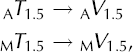
we obtain the voltage offset, ΔV, needed to correct the 1.5 m data:

This voltage correction can be applied to correct all the thermocouple measurements. We apply it by converting the thermocouple measurements to voltages using the NIST thermocouple equation, adding the correction and reconverting to temperature:

where _C V and _C T are corrected voltages and temperatures.

Figure 6 shows the corrected data in the same format as Figure 1. The change in temperature with depth follows expected trends. Temperatures at depths >0.25 m show very little variation on a daily period. The data correction is equally valid at all depths, and both the correlated (Fig. 6d) and anticorrelated (Fig. 6b) variations are removed. The 3.8°C STV shown in Figure 1c is almost completely removed in Figure 6c. All the datasets can be corrected by requiring that the temperature variations of the deep thermocouple be smooth on a weekly basis. Figure 7 compares corrected and uncorrected data for the Siple Dome dataset. The corrections are also very good in this case.

Fig. 6. (a) Corrected thermocouple data from the surface (gray dots), 0.5 m depth (gray curve with black squares), 1.0 m depth (black curve with black circles), 1.5 m depth (gray curve with black diamonds) and the reference temperature (black dots) within the unperturbed snowpack in Summit, Greenland, between 20 March and 30 April 2004. Cf. Figure 1.

Fig. 7. Siple Dome measured (gray) and corrected (black) data at 4 and 6.15 m depth.

The Origin of the STVs

Our analysis of the data suggests the source of the STVs is within the data-logger box, resulting from errors in the thermistor, wire heating or a temperature-dependent voltage offset produced within the electronics of the data logger (J₃ in Fig. 2). Perhaps in conjunction with other effects, these errors sum to create an additional signal. Reference SchraffSchraff (1996) discussed the voltage offset introduced in the internal electronics of the lOtech Daqbook data loggers, and showed that correcting for the offset changes the measured temperature by 4.7°C. These data loggers are similar to the Campbell Scientific CR10 data logger used in our experiment. Schraff does not mention any temperature dependence for the voltage offset, but it does seem likely that a temperature effect might exist. The thermistor used in the data logger in our experiment was a Campbell Scientific CR10TCRF. This thermistor is a semiconductor created to have a resistance that varies significantly as a function of temperature between −53 and 48°C. The CR10TCRF is capable of measuring temperature to better than ±0.2°C (Reference GyorkiGyorki, 2004). It may be that the signal we see in the thermocouple data is a systematic variation within the thermistor data.

Independent of the exact origin of the voltage offset, we can further explore the nature of the voltage correction by plotting it as a function of the reference temperature. This is done in Figure 8. For the Greenland data, the voltage correction varies as a simple non-linear function of the reference temperature. An eighth-order polynomial (R² = 0.98) can be used to correct the thermocouple data using only the reference temperature. Resulting corrected data are not as smooth as data corrected with the method described in the previous section. Notice that ΔV increases as reference temperature either increases or decreases from ~−32°C. This explains why the correlation of subsurface temperature shifts from correlation to anticorrelation at ~−32°C.

Fig. 8. (a) Voltage correction as a function of reference temperature for the Greenland data we collected. (b) Voltage correction as a function of reference temperature for Siple Dome data. (c) Measured voltage offset as a function of reference temperature for laboratory measurements. Note the hysteresis in (b) and (c). In each successive plot, the voltage correction/offset is about an order of magnitude less than in the previous plot. This is partly because the data loggers at Siple Dome and in the laboratory did not reach temperatures as low as the data logger at Summit Greenland.

We found a more complicated relationship between the reference temperature and the voltage correction in the other datasets. The Siple Dome data exhibit significant hysteresis, and are shown in Figure 8b. At any reference temperature the voltage correction has a single value at any given time that relates smoothly to values at adjacent times, but at significantly later times the voltage correction may be quite different for this same reference temperature. The curve loops around with time, in a typically hysteretic fashion.

The measured voltage offset and reference temperature also show strong hysteresis in our laboratory measurements. We shorted one of the channels in the data logger with a copper wire, placed the data logger in a cold room and varied the temperature of the room. Measuring the voltage across the shorted channel should give just the voltage offsets within the data logger. If there were no temperature-dependent junction voltages in the data logger, the measured voltage should be constant. In fact it was found to vary with the temperature of the data logger as shown in Figure 8c. Neither the voltage correction in the Siple Dome data, nor the voltage offset measure in the laboratory are as large as the voltage correction in the Greenland data. But the STVs observed in the Greenland dataset were also much greater than in the Siple Dome dataset, and the frequency of time variation of the Greenland reference temperature was much greater than in the Siple Dome data. The Greenland reference temperature reached much lower values than were reached in the laboratory. These could be possible reasons for the larger STVs in the Greenland data.

Discussion

Two matters warrant discussion. The first concerns how our new correction compares to other methods of correction. The second regards implications for improving data collection methods and instrumentation.

Figure 9 plots our corrected temperature at 1.5 m depth (_C T _1.5), and the uncorrected temperature at 1.5 m depth (_M T _1.5) against time. Two common methods of data smoothing are to report data averaged over 24 hours, or to apply a 5 day running mean. A curve through the 24 hour average data shows a ~9 day, 0.5°C amplitude variation in the temperature at 1.5 m depth which, by our correction, is entirely fictitious. The 5 day running mean has similar variation, but with an amplitude of 0.2°C. This false temperature variation is detrimental to attempts to use the temperature profiles to infer heat flux or snow properties, and in fact suggests the operation of entirely fictitious processes. Averaging thermocouple data is clearly a much less satisfactory method of correcting the data than eliminating physically unrealistic high-frequency temperature variations.

Fig. 9. Corrected (solid black curve) and uncorrected (light-gray dots) thermocouple data at 1.5 m depth for our Greenland dataset. Averaging the measured data over 24 hours (gray connected triangles) or applying a 5 day running mean (black connected circles) produces fictitious temperature variations with 0.2–0.5°C amplitude and ~9 day period.

Because the correction applies to all thermocouples equally, and because in one case a simple relation could be found between the temperature of the data logger and the voltage offset needed to correct the thermocouple data, it seems clear to us that the origin of the STVs is in the datalogger box. The immediate implication is that higher-quality temperature data could be collected if the data-logger box were kept at more constant temperature. This could be done with a heating mechanism, or by burying it a meter or so below the snow surface (which may have been done for some of the data shown). A second implication is that it might be possible to correct for the voltage offsets within the data logger by electronic design or by using more accurate reference thermistors.

The most important aspect of this paper, however, is its demonstration that temperature variations exist in Arctic and Antarctic thermocouple data that are related to temperature variations occurring in the box that houses the data logger. We discovered these STVs because the data we collected and analyzed showed unusually large STVs that were coherently related to the reference temperature in the datalogger box. The ambient temperature changes in our data were particularly large, being collected over the termination of the Arctic winter, and our enclosure was deployed in an exposed setting. Because the STVs were large and clear, we were able to recognize their non-physical nature, devise a way to eliminate them and also infer that they must originate from within the data-logger enclosure. Examining other datasets, we seem always to find similar, but usually smaller, STVs. Because subsurface temperature is such an important parameter in Arctic and Antarctic research, recognition of these non-physical STVs is important, particularly since, once recognized, they can be removed in a much better fashion than by simple averaging techniques.

Summary

Simultaneous non-physical temperature variations with a daily frequency exist in a number of Arctic and Antarctic thermocouple datasets. They appear to arise within the electronics housed in the data-logger enclosure. The STVs can be removed if the thermocouple temperature measurements were made over a range of depths below the snow surface, by requiring that temperatures at depth be slowly varying. The deepest thermocouple is used to calculate a correction, which, when applied to the entire array, corrects the temperature time series at all depths. Due to the slightly non-linear nature of the thermoelectric thermocouple relation, all corrections are made in voltage space and then converted back to temperature. After the STVs are removed, there may remain a temperature offset (relative to the actual temperature) of all thermocouple data. Our method does not guarantee the correct absolute temperatures have been measured, but merely removes non-physical time variations in the data in a fashion that does not appear to introduce new non-physical variations. The method of correcting thermocouple data we describe can be applied to any thermocouple data for which temperatures are measured at depths more than 0.5 m into the snowpack.