


1. The Purpose of the Paper
The presence, in polycrystalline ice, of an interconnected system of water-filled veins that lie along the lines where three grains meet was predicted by Reference Nye and FrankNye and Frank (1973) and has been observed by numerous workers. The exact equilibrium geometry of an idealized system with isotropic surface free energies has been derived by Reference NyeNye (1989). The main purpose of this paper is to study the equilibrium geometry of the vein system in ice using photographs which resolve the features and to compare the real system with the idealized system.
2. Introduction
Polycrystalline ice is a two-phase system primarily because of the limited solubility of impurities in the solid phase. A liquid phase is inevitable above the eutectic temperature once the solubility limit has been exceeded (Reference Paren and WalkerParen and Walker, 1971). Water in polycrystalline ice occurs within grains in the form of internal melt-figures and inside bubbles, at grain boundaries in lenses and along the lines where three grains meet, the grain edges. The water located at the grain edges is of primary importance as it is here that the two phases are in thermal equilibrium.
The equilibrium geometry of the water inclusions is determined by the surface free energies of the solid-solid interface or grain boundary ϒ ss and the solid-liquid interface ϒ sl. The term equilibrium geometry refers to the shape of the inclusions when there are no temperature or impurity concentration gradients within the vein system. If ϒ ss and ϒ sl are isotropic, i.e. they are independent of the crystallographic orientation of the grains, then the equilibrium geometry is defined by the dihedral angle φ, which is the angle measured in the water where the water meets a grain boundary. As ϒ ss and ϒ sl are in this case constants of the system, we can see from Figure 1 that

and ϕ is therefore also a constant. Reference Nye and FrankNye and Frank (1973) described how the equilibrium geometry depends on the exact value of ϕ They found that for ϕ > 60° the liquid phase resides in isolated pockets at four-grain intersections. When ϕ < 60°, however, the liquid phase extends along the grain edges forming an interconnected system of veins. The veins are equilateral in cross-section with almost cylindrical faces that are concave as viewed from the ice, as shown in Figure 2a. In terms of the radius of curvature r v, which, for a straight vein, is constant around the vein cross-section, the vein width d v is given by
and the cross-sectional area of the vein A v is
where ϒ = π/6 − ϕ/2. For ϕ = 32° (the value measured by Walford and reported in Reference Nye and MaeNye and Mae (1972)), Equation (3) reduces to ![]() . Four veins meet in a node at a four-grain intersection. The stable nodal shape has been computed by Reference NyeNye (1989) for a constant dihedral angle of ϕ = 33.6° (the value measured by Reference Walford, Roberts and HillWalford and others (1987)), and is a tetrahedron with concave non-spherical faces and corners that open out into the veins (see Fig. 2b).
. Four veins meet in a node at a four-grain intersection. The stable nodal shape has been computed by Reference NyeNye (1989) for a constant dihedral angle of ϕ = 33.6° (the value measured by Reference Walford, Roberts and HillWalford and others (1987)), and is a tetrahedron with concave non-spherical faces and corners that open out into the veins (see Fig. 2b).

Fig. 1. The dihedral angle ϕ where the water meets a grain boundary between two grains A and B.

Fig. 2. Vein system geometry for ϕ < 60°; (a) vein cross-section for ϕ = 32° and (b) perspective drawing of a node for ϕ = 33.6° (from Reference NyeNye, 1989).
The equilibrium geometry for isotropic surface free energies is strictly uniform; all the nodes are identical and all the veins have identical cross-sections. Anisotropy in ϒ ss or ϒ sl will produce a non-uniform equilibrium geometry and the vein system may not be complete. However, even in a non-uniform vein system, it is possible for the radius of curvature r v to be a constant of the system, if the deviations from uniform geometry are primarily due to anisotropy in ϒ ss This is because the temperature depression in the veins due to the curvature of the vein walls is proportional to ϒ sl/r v.
Similar results have been obtained for the melt geometries of other polycrystalline materials, notably for metals and alloys (Reference SmithSmith, 1948) and for silicate melts (Reference BeeréBeeré, 1975a, Reference Beeréb, Reference Beeré1981). The dihedral angles of many of these systems have been measured. (Reference BeeréBeeré 1975a, Reference Beeréb) commented that dihedral angles ϕ > 60° are typical for powder compacts and Reference SmithSmith (1948) quoted many angles ϕ > 60° found in alloys. For such systems, the melt is found in pockets at the four-grain intersections. In both these systems, the liquid and solid phases generally have different compositions. Reference McKenzieMcKenzie (1984) noted that observations of the dihedral angle in silicate and other ceramic melts are compatible with ϕ < 60° (see e.g. Reference Waff and BulauWaff and Bulau (1979) who measured ϕ ≈ 50° for silicate melts). The conclusion is that partially molten mantle rocks contain an interconnected network of veins. This is directly analogous to the situation in ice.
Some previous measurements of the dihedral angle in ice are listed in Table 1. The values show some scatter but in all cases ϕ < 60°, which suggests that there is an infinitely connected network of veins and that the idealized vein system shown in Figure 2 and described by Equations (2) and (3) is sufficient for most purposes. Reference Nye and FrankNye and Frank (1973) suggested that the presence of such an infinitely connected vein system would cause a glacier to be permeable to water and impurities. Other physical properties of ice, in particular the high d.c. conductivity of polar ice (Reference Wolff and ParenWolff and Paren, 1984) and the flow of glacier ice (Reference Paren and WalkerParen and Walker, 1971; Reference Glen, Homer and ParenGlen and others, 1977) have also been explained on the basis of a well-connected system.
Table 1. Measurements of the dihedral angle ϕ in ice

The values quoted in the table were all measured either at lenses or where a vein crops out at the surface of a sample. There are very few reported observations concerning the detailed geometry of the vein system itself. Reference Raymond and HarrisonRaymond and Harrison (1975) presented observations of the veins found in natural ice samples taken from Blue Glacier, Mount Olympus, U.S.A. They reported that not all grain edges had veins. However, they did not examine the details of the vein cross-sectional shape and were unable to resolve the vein system in sufficient detail to relate the observed width of the veins to the parameters of the vein cross-section. It is of interest to know how uniform the equilibrium geometry is, as this will fix an upper limit to the connectedness of the vein system. Other mechanisms associated with deformation processes (Reference Nye and MaeNye and Mae, 1972), blocking by bubbles (Reference LliboutryLliboutry, 1971) and thermal properties of bubbles partially filled with water (Reference RaymondRaymond, 1976) could cause further reductions.
3. Samples
Clear, stress-free polycrystalline ice samples were grown in the laboratory using the apparatus shown in Figure 3. A plastic bag filled with distilled water was lowered into a freezer. The temperature in the freezer was −27°C. The plastic bag used was made of 35 mm film cover, which could be cut to any length. A bag was created by tying a knot in one of the open ends. By freezing the water unidirectionally in this way, the volume expansion on freezing was accommodated and the ice was left stress-free. The ice/water interface or freezing front remained in roughly the same position relative to the freezer; it swept through the sample as the bag was lowered. The air that was dissolved in the water came out of solution at the freezing front. By stirring the water just above the freezing front, the bubbles were dislodged from the ice/water interface and so did not become entrapped in the ice. The ice was therefore largely bubble-free and hence clear. The depth of the stirrer could be altered. This was important because the freezing front tended to rise by a few centimetres relative to the freezer as the bag was lowered into it and the reservoir of warm water above the interface was lost. The resulting ice columns were typically about 45 cm long and 3.2 cm in diameter.
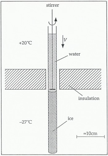
Fig. 3. Sample-growing technique.
Some ice columns were grown very slowly at about 4 cm d−1. This usually produced a single crystal with c-axis normal to the direction of growth. Reference Ketcham and HobbsKetcham and Hobbs (1967) specified a maximum speed of about 7cm d−1 for growing a single crystal. As veins only exist in polycrystalline ice, the majority of ice columns were grown at about 15 cm d−1. The grains in these columns tend to be long and thin with the majority of veins running roughly parallel to the cylinder axis. At the end of the columns, the ice was often a single crystal with the c-axis normal to the direction of growth. The grain-size in the direction of growth varied from less than 1 mm to about 400 mm. The grain-size perpendicular to the direction of growth was seen to increase with height in the column, typically from about 1 mm up to 10 mm. The grain structure in the ice columns therefore shows strong signs of competitive grain growth. The preferred orientation of crystals has the basal plane parallel and the c-axis normal to the direction of growth, in agreement with observations by other workers(Reference RamseierRamseier, 1966, Reference Ramseier1968; Reference Ketcham and HobbsKetcham and Hobbs, 1967).
The distribution of the ionic impurities in the columns was investigated by measuring the electrical conductivity of meltwater samples taken from different regions in the columns (Reference MaderMader, 1990). Most of the impurities were found at the ice/bag interface, within about 1 mm of the curved surface, and at the very top of the columns. Impurity-concentration analyses were carried out by British Antarctic Survey chemists on a melted sample of polycrystalline ice taken from the central part of an ice sample, the dirty surface layer having been melted away. They measured a bulk impurity content of about 10−6 mol 1−1.
The ice columns were split into samples, 5–7 cm long, by making an incision around the circumference of the column with a fine-bladed saw. The sample was then cleaved off the column by placing the tip of a heavy-duty, fiat-bladed screwdriver in the incision and giving it a sharp tap with a hammer. The surfaces were generally flat and clean.
The veins in the samples immediately after growth were very small because of the low temperature in the freezer (−27°C). The veins were best studied when they were much larger, that is, at temperatures closer to 0°C. Therefore, in preparation for an experiment, the temperature of the samples was raised by placing them in a vacuum flask that contained a freezing mixture of singly-distilled water and distilled-water ice chips. The samples were each in individual, scaled plastic bags and so were only in thermal contact with the ice/water mixture. This preparation process we called rotting, and has been discussed in more detail by Reference NyeNye (1991b) and Reference MaderMader (1992).
The temperature of the freezing mixture was very close to 0°C. It was probably marginally below 0°C because of residual impurities in the flask. As the temperature of the sample rose, the veins grew. Eventually, the veins were very large. Apparent vein widths of several 100 μm have been measured in samples that had been rotted for periods of weeks. Initially, the veins grew fast but, by the time they reached widths of 100 μm or more, the process was much slower. The samples could be kept for many days at this stage with very little change in the vein size. The longest a sample was held like this before use was 70 d.
4. Experimental Apparatus
The experiments were performed in a commercial walk-in freezer that was controlled to 0° ± 2°C. Figure 4 gives an overview of the experimental apparatus used inside the freezer. A cylindrical, polycrystalline ice sample S (length ≈ 7 cm, diameter ≈ 3 cm) was suspended in a saline water bath A (capacity ≈ 1.5 1). The ice was clamped in the jaws of a sample holder H that was specially designed to hold and position ice. The sample was viewed in transmission by an optical microscope M which has an attachment for a camera (not shown). Light was provided by a white-light source L (power ≈ 15 W)and directed through the sample into the microscope using a surface-silvered mirror R. A water-filled chamber F (thickness ≈ 3 cm) was placed between the light source and the mirror to act as an infra-red filter and prevent unwanted heating and melting. The apparatus was mounted on an anti-vibration table which consisted of a very heavy piece of slate (51 cm × 104 cm × 4 cm) that was separated from the basic table by four small partially pumped-up bicycle inner tyres.
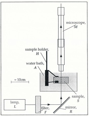
Fig. 4. Schematic representation of the experimental apparatus.
The sample holder Η had to be capable of holding a piece of ice immobilized for the duration of an experiment (about 30 min), so that the same vein remained within the field of view of the microscope throughout. The problem with most holding devices is that they induce pressure melting of the ice at the point of contact. A layer of water builds up between the ice and the holder causing slip. One solution to this problem, suggested by Dr M. Walford, is to use porous glass pads in contact with the ice. No slip occurs as the meltwater created by the pressure melting flows into the porous glass and so the pad remains in contact with the sample.
The sample holder used is shown in Figure 5. It has three porous glass pads, each bonded by an epoxy resin on to a flat spring. The springs are attached to a stage that allows the cylindrical ice sample, up to 5 cm in diameter, to be rotated about its axis. There is a second rotational facility about an axis which is also in the horizontal plane but is perpendicular to the first. The angle of each rotation can be independently determined to within ±1°C. Each rotation stage is a miniature crown-wheel and pinion with the pinion connected to a rod that extends out of the water bath. By turning the rods, the pinion rotates the crown wheel and hence the sample. Rotations about the vertical axis and translations in the horizontal plane were possible to a limited degree by rotating the stand on the table. Translations in the vertical direction were effectively achieved by the focusing of the microscope. The micro-manipulator therefore allowed three rotations and three translations, though not all had the same degree of control or the same range.

Fig. 5. The sample holder.
The microscope M used was of the most basic kind and consisted merely of an objective lens and an eyepiece lens or camera lens. It was focused using the eyepiece, which was then removed and replaced by the camera so that a photograph could be taken. The distance from the plane of focus to the lens is roughly the same as the diameter of the samples (about 3 cm) so that the microscope could scan all the way through. The final magnification on the negative was about ×l5. Measurements were taken off prints rather than directly off the negatives themselves. The maximum degree of enlargement available was about ×12, giving a total magnification of the object of up to ×180. To determine the magnification, a photograph was taken of a calibration disc which showed 1 mm intervals. The negative was then placed in the enlarger before and after prints were made. The total magnification was determined to within about ±0.5%.
Distances between two lines on a print can be determined to within about ±0.25 mm, i.e. about 1.4 μm at maximum magnification. This is therefore the resolution limit and is a consequence mainly of the graininess of the negative. Veins with apparent widths of less than about 3 μm therefore could not be resolved, as the vein edges start to overlap on the negative at this stage. Also, diffraction effects start to become important for such small veins.
5. Temperature Control of Wellrotted Samples
Observations of the geometry of the vein system are best conducted on heavily rotted samples when the veins are very large. It is important that the vein size does not change during the course of an experiment. As the vein size is a function of temperature, the samples must be held in a thermally stable environment.
In a two-phase system, temperature changes involve both specific and latent heats. Consequently, polycrystalline ice has a markedly different thermal behaviour from that of singly crystalline ice. Reference NyeNye (1991a) derived a diffusion equation for polycrystalline ice in terms of an effective specific heat σ eff (Reference HarrisonHarrison, 1972) which contains two terms: a constant term that describes the specific-heat contribution and a second term that is due to the latent-heat contribution and is strongly temperature-dependent. As the temperature in a sample approaches 0°C, the veins melt and the latent-heat contribution starts to dominate the heat flows. σ eff becomes very large and therefore so does the time constant for a unit change in temperature.
Heavily rotted samples are in the region where σ eff is several orders of magnitude greater than for cold polycrystalline ice or for a single crystal. For these samples, this is the case when the temperature in the sample is greater than −10−30C. The time constant for changes in temperature within this region is large compared with the time necessary to perform an experiment. This means that, provided the temperature at the surface of the sample can be maintained at some value greater than −10−30°C but below 0°C, the veins will be stable for the duration of an experiment. It is not necessary for the exact temperature depression in the sample to be known.
The easiest way to create a very small, constant temperature depression at the surface of the sample is to exploit the effect of the saline environment of the water bath. If an ice sample is in contact with a large, well-stirred reservoir of saline solution, that is at some temperature above 0°C (measured well away from the sample), then the combined effect of the salinity and temperature in the bath causes continual melting at the sample surface. The temperature at the surface of the sample is therefore, by definition, the melting point of the two-phase system, which is a function of the impurity concentration in the bath and the curvature of the ice surface and is below 0°C. There is a temperature gradient at the sample surface. The heat which flows down this gradient from the bath, which is above 0°C, to the sample surface, which is below 0°C, does not raise the temperature of the sample but provides the latent heat of melting at the sample surface. The gradient is maintained, if the bath is well-stirred and the volume of water is large compared to the sample size. The temperature depression at the sample surface is constant until the sample has melted away.
The samples were observed whilst in contact with a solution made up from chilled, distilled water with a very small amount of NaCl. No attempt was made to determine the exact impurity concentration in the bath. It is important that the bath should not be too warm so that the sample does not melt away too quickly.
6. Vein Optics
The optical observations of veins previously reported do not resolve the veins in sufficient detail for the observed width to be related to the other quantities associated with the cross-sectional area. However, if the veins are large enough, it is possible to get very detailed pictures of the vein system.
A typical example of a photograph of a rotted node is shown in Figure 6. For comparison, Figure 2b shows one of Nye’s computer-generated perspective drawings of a node. The computed shape is drawn as if the node were a solid opaque structure made up of four surfaces, the ice faces, of which only two are completely visible in the drawing. The photograph, by contrast, shows all features because the veins are actually transparent to visible light; each of the four veins is indicated by three lines, namely the vein edges. There are six such vein edges associated with every node, as each vein edge is shared by two veins. All six vein edges are visible in both the photograph and the drawing.

Fig. 6. Photograph of a rotted node.
If the veins are equilateral in cross-section, the distances between the three lines on the photograph allow one to deduce the true width of the vein d v from the equation:
where the orientation angle Ω is given by

and a, x and Ω are defined in Figure 7.
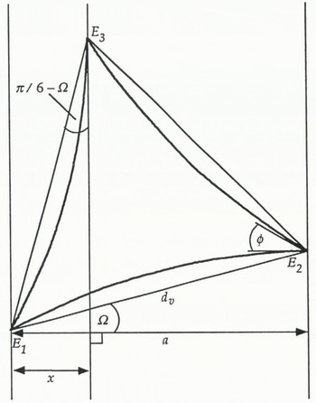
Fig. 7. Vein cross-section for an equilateral vein with dihedral angle ϕ = 32° at an angle Ω to the plane of focus and showing the apparent vein width a.
There is a need to understand the photograph in more detail because the vein edges are not always well defined and it is necessary to know where the vein width starts and finishes. The reason we can see the veins at all is because they refract light; viewed side on, the water-filled veins act as tiny triangular-shaped prisms with a refractive index slightly greater than that of the surrounding ice. The diagrams in Figure 8 show a simplified version of the ray optics (not to scale). The vein cross-section is approximated by an equilateral triangle with flat sides, i.e. r v = ∞. Two orientations of vein are shown.

Fig. 8. Ray diagrams for simplified (flat-sided) vein cross-sections.
The plane of focus of the microscope is perpendicular to the direction of the light and can be at any height in the drawing. From Figure 8 we can see that if the plane of focus is above the vein (i.e. on the microscope side), the outer vein edges appear dark and the central vein edge bright. Conversely, if the plane of focus is below the vein (i.e. on the lamp side), the outer vein edges appear bright and the central vein edge dark. The thickness of the lines is a measure of how far away from the plane of focus a particular edge is located. Also, and most importantly, the diagrams show us how to measure the apparent vein width a. It must be measured to include dark outer lines or exclude bright outer lines. The central vein edge is, for both cases, in the middle of the central line.
The patterns of light and dark rays and the rules about how to measure the apparent vein width are similar for, all orientations of veins. They are not affected by introducing a finite radius of curvature. Symmetry about the central line can only be expected for symmetrical orientations, such as the ones shown here. However, for non-symmetrical orientations, if the central vein edge is not very far from the plane of focus, the line is narrow. Under such circumstances, the position of the central vein edge with respect to the outer vein edges is well defined. Note that it is not necessary for the vein to lie in the plane of focus for the vein width to be determined. In fact, where a particular vein edge cuts across the plane of focus, it is invisible.
The node in the photograph of Figure 6 can now be described in more detail, although the description remains qualitative. In the orientation shown, veins 2 and 3 are more sharply inclined with respect to the plane of focus than veins 1 and 4. Vein 1, in fact, lies almost in a plane parallel to the plane of focus. The node conforms at least qualitatively to the tetrahedral shape expected. Veins 1 and 3 are angled away from the microscope and veins 2 and 4 are angled towards it.
7. Observations of Non-Uniform Vein-System Geometry
Deviations from uniform equilibrium geometry have been routinely observed during the course of this work. Figure 9 and 10 show a representative selection of veins and nodes.

Fig. 9. Examples of observations of non-uniformity in the vein-system geometry, (a) Shows a series of four nodes, all of which have pinched-off veins. Node 1 has only one pinched-off vein but nodes 2–4 each have two pinched-off veins. Note that some spikes extend along the grain edge further than others, (b) Shows a vein running into a node at which the other three veins are pinched-off. The vein system terminates at this node, (c) Shows another example of a node with two pinched-off veins, (d) There are two nodes in the picture, one behind the other, and the view is down the interconnecting vein. The vein cross-section is clear to see and it is evidently not equilateral.

Fig. 10. Examples of irregular nodal structures. (Note that in (c) one of the veins pinches off leaving a series of pods along the grain edges. A similar observation in natural ice has been reported by Reference Raymond and HarrisonRaymond and Harrison (1975).)
The most obvious indicator of a non-uniform equilibrium geometry is the occurrence of pinched-off veins in an otherwise interconnected system. The absence of veins on some grain edges in natural ice was first noted by Reference Raymond and HarrisonRaymond and Harrison (1975). Figure 9a, b and c show examples of such phenomena in the laboratory-grown ice crystals. A less-extreme indicator of a nonuniform vein system is the observation of non-equilateral vein cross-sections, e.g. Fig. 9d.
The most frequent observation that implies a nonuniform equilibrium geometry is that of nodes where the apparent vein widths of the four veins meeting there are very different. Figure 10 shows three examples. The radius of curvature calculated for the four different veins of each node assuming an equilateral vein cross-section are different.
In the laboratory-grown ice, non-uniform nodes are the norm. During the course of this research, photographs of a total of 43 nodes that have continuous veins along all four grain edges have been taken. These photographs were collected over 3 years and not according to any criteria and so may be viewed as a random sample. Twenty-three have veins with apparent vein widths that differ by a factor of 2 or more. Only seven can be described as uniform, that is, the idealized, isotropic equilibrium geometry, when applied to each vein, gives the same value for r v, to within the error. The remaining 13 have veins with distinctly different apparent vein widths, but the variation is less than a factor of 2.
Also, in some samples, a high number of pinched-off veins was noted; as many as 10% of the nodes had one or more pinched-off veins, i.e. at most 5% of veins were absent. Nodes with three pinched-off veins are very rare. A node where all four veins are pinched-off, that is, a pocket of water at a four-grain intersection, has not been observed. The interpretation of these observations is given in section 10.
8. Experimental Techniques
The method for establishing the vein cross-section of a non-uniform vein in terms of the three vein widths d v1, d v2 and d v3 is straightforward. The vein is photographed from two different directions. We then have two projections of the vein with a known angle θ between them. In Figure 11, l 1 and l 2 represent the first projection and l 3 and l 4 the second. Looking at the construction triangle E2E5E3, we can see directly that the sides are given by

Using the law of cosines, we get for d v1

Similarly, d v2 can be calculated using the construction triangle E3E6E1, and d v3 using E1E4E2. The angles Φ 1, Φ 2 and Φ 3 can then be calculated directly, using the law of cosines, in terms of these vein widths.
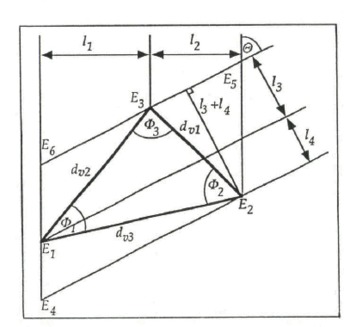
Fig. 11. Sketch showing two projections of the vein edges of a non-equilateral vein and the three vein widths. The vein cross-section itself is not shown.
The ice must be carefully observed during the rotation, so that we know how the vein edges have moved relative to each other and hence where they are in the construction. Note that the construction shown in Figure 11 only applies for rotations during which the central vein edge changes places with an outer vein edge. Where this is not the case, the construction must be altered to suit, although the method remains essentially the same.
To define the vein cross-section completely, it is necessary to measure the dihedral angles. It is possible to get a direct observation of the dihedral angles at the vein edges by orienting the sample so that the line of sight is coincident with the axis of the vein, such as in Figure 9d, in which case the complete vein cross-section can be seen. Generally, however, the veins are long and not perfectly straight and so the cross-section viewed in this way is often too blurred to allow the dihedral angles to be measured.
This problem can be overcome by exploiting the tetrahedral geometry of a node. When the sample is rotated so that two veins, which meet at a node, are superimposed when viewed through the microscope, the dihedral angle of the vein edge common to them both is visible. It is important for this vein edge to be brought to a cusp to obtain a valid measurement of the real dihedral angle. The motion of the vein edges as two veins are superimposed is illustrated in Figure 12a–c. The vein edges of vein 3 are drawn as dashed lines merely to avoid confusion, so that it is clear where all the vein edges are. In Figure 12c, the dashed and the unbroken lines should be superimposed. The fine line f that runs down veins 1 and 2 into the dihedral angle is clearly visible on the photographs. It is not a vein edge but occurs because of refraction at the curved surfaces of the node. It shows where the line of sight is tangential to the curved surfaces and has no other physical significance.

Fig. 12. Three sketches of a node illustrating the motion of the vein edges as (a) a typical view is rotated through (b) an intermediate stage to (c) the final stage where veins 3 and 4 are superimposed and the dihedral angle ϕ of the vein edge common to these veins is visible. The vein edges of vein 3 are drawn as dashed lines to avoid confusion.
The dihedral angle will only be constant along the vein edge common to two veins if the solid-liquid interfacial energy ϒ sl is also constant. This, in turn, implies that, for a straight vein, the radius of curvature r v is constant around the cross-section. It is possible to calculate this value of r v. From Figure 13 we have at point E3
Now


Fig. 13. Cross-section of a non-equilateral vein. In this diagram, rv1 ≠ r2 ≠ rv3 which implies anisotropy in both ϒss and ϒsl.
Combining Equations (8) and (9) gives

For isotropic γs1, r v1 = r v2 = r v3, and so putting T v1 = T v2 = r v and solving for r v we get

Now, Φ 3 = f(d v1, d v2, d v3) and so r v = f(d v1, d v2, d v3, ϕ 3). Similar equations can be developed for r v in terms of Φ 2, Φ 2 and Φ 1, ϕ 1 Therefore, all three sides and at least one angle must be known if the radius of curvature is to be calculated. Independent measurements of two of the dihedral angles allow r v to be calculated twice and so the assumption of isotropic ϒ sl can be checked for the vein in question.
9. Results
9.1. Measurements of Vein Widths
A typical result is shown in Figure 14. The vein observed ran roughly parallel to the axis of the cylindrical sample. The first projection had distances of 132 ± 1 μm and 168 ± 1 μm between the central and outer vein edges as shown in the figure. The sample was then rotated by 50° + 1° about its axis and another photograph was taken. This second projection had distances of 88 ± 1 μm and 80 ± 1 μm between the central and the outer vein edges. The sample was rotated back to the initial position and the vein photographed again. No change in the vein size had occurred during the experiment. The widths of this vein are d v1 = 185 ± 4 μm, d v2 = 261 ± 5 μm and d v3 = 334 ± 7 μm which means that they vary by a factor of 1.8.

Fig. 14. Construction of the vein widths of a non-equilateral vein cross-section from two projections of the veins. The vein cross-section itself is not shown.
9.2. Direct Observations of Dihedral Angles
An example of a typical observation on a regular node is shown in Figure 15. Typical values appear to be in the region 30° < φ < 40°. The smallest angle measured was ϕ = 25° ± 1° (Reference MaderMader, 1990), in agreement with the most recent measurement by Reference Walford and NyeWalford and Nye (1991).

Fig. 15. Observation of a typical dihedral angle in ice. The node shown in (a) is rotated so that veins 2 and 3 are superimposed in (b) showing the dihedral angle of the shared vein edge ϕ = 32° ± 1°. (N.B. The elliptical features in (a) are lenses in the grain boundary which is bounded by the vein edge that runs from vein 1 to vein 3. When the node is rotated as in (b), this grain boundary is virtually parallel to the plane of the paper. The lenses are now seen in plan view and hence appear circular. For more details on the geometry and optics of lenses, see Reference Walford, Roberts and HillWalford and others (1987).)
The dihedral angles of pinched-off veins are of particular interest. Figure 16 shows a sketch of part of the vein system seen in one of the ice samples. There are two pinched-off veins, leaving four spikes. They have one grain boundary in common, which is bounded on one side by the vein edge E. The dihedral angle at this grain boundary was measured at the spike S. Figure 17a is a photograph of the spike S. The photograph is taken from a slightly different perspective angle compared to the sketch in Figure 16. As a result, only two of the four spikes are properly visible; the third can just be seen at the very top of the photograph but the fourth spike is obscured. Figure 17b shows the view with the spike S superimposed on the vein V. The spike is quite faint and to see it requires close observation. The dihedral angle is very large, ϕ E = 105° ± 1°, and so this must be a very low-energy grain boundary. This value also explains why some of the grain edges around this grain boundary have veins whilst others do not. It was noted that, in a system with uniform geometry and constant ϕ, the veins would pinch off for ϕ > 60°. In a system with non-uniform geometry, where each vein has three different dihedral angles, ϕ 1, ϕ 2 and ϕ 3, thermal equilibrium still requires that the three sides are all convex or all concave. The condition for a non-uniform vein to pinch off is then ϕ 1 + ϕ 2 + ϕ 3 180°. If ϕ 1 = ϕ E = 105° ± 1°, then the vein pinches off when ϕ 2 + ϕ 3 > 75°. As the most common values for ϕ are in the 30–40° range, ϕ 2 + ϕ 3 could quite easily be either above or below 75°.

Fig. 16. Sketch of part of the vein system seen in one of the ice samples showing two pinched-off veins leaving four spikes.

Fig. 17. The dihedral angle at a pinched-off vein, (a) Photograph of the spike S; (b) View with spike S and vein V superimposed. The dihedral angle is φ = 105° ± 1°.
9.3. A Detailed Study of a Node
Four of the six dihedral angles of the node shown in Figure 18 were measured. In the following, E14, for example, denotes the vein edge that is common to veins 1 and 4. The dihedral angle ϕ 14 is that measured at E14 when veins 1 and 4 are seen to be superimposed. The measured angles were: ϕ 14 = 35° ± 1°, ϕ 34 = 32° ± 1°, ϕ 3 = 34° ± 1° and ϕ 13 = 39° ± 1°. ϕ 24 could not be measured because the photograph was too blurred. ϕ12 was not measured because the sample holder entered the line of sight and so obstructed the view at the required orientation. Figure 19 shows the construction of the vein widths for veins 1 to 3 from two projections of the veins. The values are shown in Table 2. The error on the vein widths is typically ±3% ≈ ±3μm. Despite the generally uniform appearance of the node, both the dihedral angles and the vein widths vary significantly.

Fig. 18. Node studied in section 9.3.

Fig. 19. Constructions of the cross-sections of (a) vein 1, (b) vein 2 and (c) vein 3 of the node shown in Figure 18.
Table 2. Vein widths for veins 1, 2 and 3 from the constructions shown in Figure 19

We have values for all three widths of veins 1, 2 and 3, as well as two of the dihedral angles of vein 1 (ϕ 13, ϕ 14), one of vein 2 (ϕ 23) and all three of vein 3 (ϕ 13, ϕ 34, ϕ 23). We can therefore calculate r v six times. The values are shown in Table 3. All six values are the same to within the experimental error and so ϒ sl may be assumed constant for this node. The variations in the vein widths and the dihedral angles are therefore thought to arise primarily from anisotropy in ϒ ss. The mean radius of curvature is r v = 269 ± 14 μm. This value is used to construct the vein cross-sections in Figure 19. ϕ 12 and ϕ 24, which could not be measured, can be deduced from the cross-sections. We get from the cross-section of vein 1, ϕ 23 = 33° ± 1°, and from the cross-section of vein 2, ϕ 12 = 32° ± 1° and ϕ 24 = 38° ± 1°. The two values of ϕ 12 are within the error of each other which adds support to the constructions.
Table 3. Values for the radius of curvature of the node in Figure 18 calculated assuming constant ϒ sl and using Equation (11)

All values ±30%.
10. Discussion and Conclusions
The observations presented here show conclusively that the vein-system geometry in the laboratory-grown samples is not uniform. Pinched-off veins, veins with non-equilateral cross-sections (the vein presented in section 9.1 has widths that vary by a factor of 1.8) and dihedral angles in the range from 25° ± 1° to 105° ± 1° have been measured. The data presented in section 9.3 are consistent with the assumption of isotropy in the solid-liquid interfacial energy ϒ sl They thus imply that the variations in the dihedral angles and vein widths are a consequence of anisotropy in the grain-boundary energy ϒ ss, and that therefore the radius of curvature rv is constant over the vein faces. However, this result only concerns the limited range of crystallographic orientations exposed over the surfaces of the node shown in Figure 18. Also, the node happens to be particularly regular in appearance, and the method itself is not very sensitive as the large error (±30%) on the values ofr v in Table 3 indicates. Further measurements are needed before we can generalize this result.
The method of measuring dihedral angles used here is preferable to observations of vein outcrops such as those of Reference MorrisMorris (1972) and Reference Ketcham and HobbsKetcham and Hobbs (1969) for two reasons:
-
1. Veins are not generally normal to the surface and so, at the outcrop, some plane section through the vein at an acute angle to the vein axis is observed. The outcrop will only be a vein cross-section when the vein axis happens to be normal to the surface.
-
2. The vein cross-section at the outcrop will not be the same as the vein cross-section in the interior of a sample because of the flaring of the vein near the surface. At an outcrop, the curvature parallel to the vein axis is large and so the curvature around the vein cross-section 1/r v is reduced to maintain a constant total curvature.
The dihedral angle ϕ was typically in the range 30–40° with much larger values (and also some smaller values) observed in a small but significant number of cases. If the variations in ϕ are due to anisotropy in ϒ ss alone, then the observations suggest that the grain-boundary energy as a function of misorientation of the grains has a plateau value with cusps at special misorientations where ϒ ss is low and hence ϕ is large.
There has been speculation in the literature concerning whether or not a glacier is permeable to water because of the existence of the vein system. Deformation, recrystallization and blocking by bubbles might cause glacier ice to be impermeable. The samples in these experiments are not subject to any of these processes and so are at maximum permeability. The non-uniformity of the vein system is the only mechanism which can limit the permeability. The observations have shown many instances of pinched-off veins; however, even in samples where many absent veins were noted, they did not amount to more than about 5% of the total.
It is possible that the number of pinched-off veins is exaggerated in these samples because of the way they were grown. It has been mentioned, that, when ice is grown from the melt, competitive grain growth occurs. The preferred crystal orientation is one in which the c-axis is perpendicular and the basal plane is parallel to the direction of growth. The method of growing the samples therefore tends to produce many low-energy grain boundaries and hence large dihedral angles, thereby increasing the probability of pinched-off veins. This also occurs in natural ice grown from the melt such as in lake ice (see e.g. Reference KnightKnight, 1962). Also, recrystallization processes in glaciers and ice sheets lead to a coarsening of the grains and therefore most likely to an increase in the number of low-energy boundaries.
In natural temperate ice, pinched-off veins arising from the non-uniformity of the vein system will provide an additional mechanism to those suggested by Reference LliboutryLliboutry (1971), Reference Nye and MaeNye and Mae (1972) and Reference RaymondRaymond (1976) which might limit the permeability. To determine whether or not a temperate glacier is permeable, we need to know what the probability p is for a grain edge to have a continuous, unblocked vein lying along it, taking account of all of the above effects. The problem then is one of bond percolation in say a diamond lattice. The bonds represent the veins which meet in nodes at four-grain intersections with roughly tetrahedral coordination. The lattice is permeable if an infinitely connected system of bonds exists. Reference Frisch, Hammersley and WelshFrisch and others (1962) studied the probabilities in such a lattice (the diamond lattice) using Monte Carlo computer simulations of the percolation. By contrast, the results of Reference Sykes and EssamSykes and Essam (1964) were achieved using series methods. Both approaches produced similar results. An infinite network exists for p > 0.39 but it does not include all the open bonds until p > 0.6. No data are available at present from which we might estimate the value of p in natural temperate ice. To do this, we would have to take account of the non-uniform vein system as well as the other limiting mechanisms suggested in the introduction. It seems unlikely that in general p < 0.39, and so temperate ice is probably to some extent permeable. However, p < 0.6 might be true, at least in certain regions of a temperate glacier, in which case the glacier may only be permeable over short distances, depending on the exact value of p.
Acknowledgements
I am grateful to Professor J. F. Nye and to Dr M. Walford for their help, advice and encouragement throughout this project. My thanks are also due to the staff of the British Antarctic Survey for performing the impurity analyses on my meltwater sample. Much of the equipment was built by Mr K. Dunn, Mr R. Exley and Mr F. Porter. Special thanks are due to Mr K. Dunn for his advice on constructional matters during the design stage and to Mr G. Keene for advice on photographic techniques. This work was supported by a grant from the U.K. Natural Environment Research Council.
The accuracy of references in the text and in this list is the responsibility of the authors, to whom queries should be addressed.


