


Introduction
Chronological control of ice-core records is of crucial importance for correct interpretation of the determined physical, biochemical and chemical proxies. Annual-layer counting of seasonal variations in chemical species and oxygen isotope ratios (δ18O) is a powerful method (Reference DansgaardDansgaard, 1964) but cannot always be successfully applied to alpine glaciers (Reference Schwikowski, Brütsch, Gäggeler and SchottererSchwikowski and others, 1999, Reference Schwikowski, Eichler, Jenk and Mariani2014; Reference OlivierOlivier and others, 2006) because it requires a near-homogeneous accumulation rate throughout the year (Reference EichlerEichler and others, 2000). The use of absolute time markers (e.g. Sahara dust horizons and the AD 1963 3H peak), as well as radiometric methods such as 210Pb, radiocarbon from carbonaceous aerosol particles (Reference JenkJenk and others, 2009; Reference SieglSiegl and others, 2009) and accelerator mass spectrometry dating, all contribute to the development of robust depth–age models for alpine glacier ice cores. In this context, biological proxies have been considered with varying degree of success. For instance, snow algae have proven to be useful for detecting seasonality (Reference UetakeUetake and others, 2006), but are of limited applicability for ice-core dating, as after 8 years they have been shown to endure autolysis and bacterial decomposition (Reference Yoshimura, Kohshima, Takeuchi, Seko and FujitaYoshimura and others, 2000). Cyanobacteria, bacteria and fungi are easily transported downwards by meltwater percolation due to their small size (Reference UetakeUetake and others, 2006). Moreover, according to Reference UetakeUetake and others, (2006), bacteria and fungi seem able to grow within the deeper strata even after their deposition, thus altering the seasonal signal. In contrast, palynological analyses of snow and ice samples have revealed that pollen retains a high potential for ice-core dating (Reference NakazawaNakazawa, 2004; Reference NakazawaNakazawa and others, 2005; Reference UetakeUetake and others, 2006; Reference SantibañezSantibañez and others, 2008; Reference NakazawaNakazawa and others, 2011, Reference Nakazawa, Konya, Kadota and Ohata2012), providing information about the paleo-environments and past atmospheric circulation (Reference BourgeoisBourgeois, 2000; Reference Liu, Reese and ThompsonLiu and others, 2005, Reference Liu, Reese and Thompson2007; Reference Yang, Tang, Bräuning, Davis, Shao and JingjingYang and others, 2008). The use of pollen as a chronological constraint presents clear advantages, some of which are specifically associated with alpine glaciers. First, plants have distinct flowering periods from spring to late summer/fall, allowing us to link the snow/ice layers entrapping the corresponding pollen with a precise flowering season. Consequently, layers with a pollen content <5 grains cL−1 are most likely to represent winter accumulation (Reference Haeberli, Schotterer, Wagenbach, Haberli-Schwitter and BorthenschlagerHaeberli and others, 1983). Pollen deposition occurs independently of precipitation, because pollen is also deposited when no snow/rain deposition occurs. In addition, since alpine glaciers are normally located within a few km of the pollen source, samples as small as 10 mL usually contain a sufficient amount of pollen grains to perform the analyses (Reference NakazawaNakazawa and others, 2005, Reference Nakazawa2011). In contrast, in arctic ice the minimum sample volume required is 1 L (Reference McAndrewsMcAndrews, 1984; Reference BourgeoisBourgeois, 2000).
Reference NakazawaNakazawa (2004) and Reference NakazawaNakazawa and others, (2005, Reference Nakazawa2011) explored the possibility of using seasonal taxonomic variation of the pollen spectra as a time control on a mid-latitude glacier firn core retrieved from the Russian Altai. Although these studies are based on only three pollen types (Pinaceae, Betula and Artemisia), they showed that pollen variability in ice provides a good indication of the seasonality and helps to set annual boundaries. Based on these encouraging results we aimed to further develop the potential of palynological studies on ice cores by developing a different methodological approach.
The present paper presents a novel statistical approach to define seasonality. It is based on accurate taxonomical identification and quantification of pollen content, and is supported by a daily modern pollen-monitoring technique. This palynological method has been developed on ice samples from a 10 m firn core collected from Alto dell’Ortles glacier, a mid-latitude alpine glacier located in the Eastern Alps (Fig. 1). The aim of the analyses was to determine the presence and composition of pollen content in the firn core, to quantify it and to detect the annual and interannual variability of the pollen spectra to ultimately establish a pollen-based timescale. The method has been developed as a base for future research on the 75 m long ice cores extracted from Alto dell’Ortles during fall 2011 (Reference GabrielliGabrielli and others, 2012).
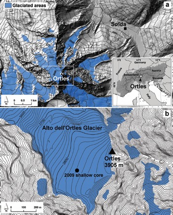
Fig. 1. (a) Geographical setting of Ortles mountain and of Solda aerobiological station. (b) Close-up of Alto dell’Ortles glacier, where the 2009 shallow firn core was retrieved.
Study Area
Alto dell’Ortles glacier (46°30′32″ N, 10°32′41″ E) is located in the Eastern Alps close to the border between Italy, Austria and Switzerland (Fig. 1). It covers a total surface area of 1.04 km2 at 3018–3905 m a.s.l. on the northwestern slope of Ortles mountain (3905 m a.s.l.), making it the highest glacier in the Eastern Alps. The maximum ice thickness in the upper part of the glacier is ∼75 m (Reference GabrielliGabrielli and others, 2012), presenting an excellent lamination of the exposed ice layers down to bedrock (Reference GabrielliGabrielli and others, 2010).
From a climatic perspective this area is characterized by a continental precipitation regime with exceptionally low mean annual precipitation, reaching minimum values of 440–530 mm a−1 north of Ortles mountain, in the Vinschgau valley (Reference FliriFliri, 1975). This region is indeed characterized by a so-called ‘dry inner alpine’ climate. Here the treeline is located at ∼2100 m a.s.l. and is formed by Pinus cembra (arolla pine) and Larix decidua (larch) forest. Above this altitude, Pinus mugo (mountain pine) stands and Alpine grass mats predominate (Reference PeerPeer, 1995).
Methodology
Pollen analyses of snow samples
In June 2009 a first extensive glaciological survey was performed on Alto dell’Ortles glacier at 3830 m a.s.l., where a 10 m shallow core was collected by drilling with a lightweight hand auger. The shallow core was divided into samples of ∼10 cm length, which were transported, frozen, to the University of Venice. The samples were cut in half cross section in a cold room, melted in a class 1000 clean room and poured into 1 L low-density polyethylene (LDPE; Nalgene) plastic bottles (Reference GabrielliGabrielli and others, 2010).
From each sample an aliquot of ∼35 mL was dedicated to pollen analyses, performed at the University of Innsbruck. Here the entire aliquots were processed with acetolysis (Reference ErdtmanErdtman, 1960), the pollen content was concentrated by hydro-extraction (centrifugation) and then prepared in glycerine as is standard procedure in fossil pollen analyses (Reference Faegri and IversenFaegri and Iversen, 1989). In contrast to Reference NakazawaNakazawa and others, (2011), whose analyses were based on three pollen types (Betulaceae, Pinaceae and Artemisia), here the complete pollen content of the samples has been identified and quantified, in order to enable a better definition of the seasonal pattern and to allow more detailed statistical analyses. In fact, a complete pollen spectrum contains much information about seasonality and allows us to avoid misinterpretation of absence/presence of a single pollen taxa. For example, if in a sample deposited during late summer a pollen type typical of late summer is missing, the pollen spectrum will still provide the seasonal information as it contains other taxa that also flower in late summer.
Pollen identification was performed using a light microscope at 400× and 600× magnification, using the reference collection of the Institute of Botany, University of Innsbruck, as well as standard identification keys (Reference Moore, Webb and CollinsonMoore and others, 1991; Reference Faegri, Iversen, Kaland and KrzywinskiFaegri and others, 1993; Reference BeugBeug, 2004) and a pollen atlas (Reference ReilleReille, 1992). Pollen grains, microcharcoal and non-pollen palynomorphs (NPPs) were quantified using the Online Pollen Counter (OPC; Reference LawtonLawton, 2010), an application that allows faster counting by replacing manual counting. OPC includes a reference catalogue of European pollen and non-pollen palynomorphs and provides pollen count files that can be downloaded and/or stored in a database. The application has been developed by the Institute of Botany, University of Innsbruck, and is accessible only by members of the institute. Finally, the pollen diagram was drawn with C2 software by Reference JugginsJuggins (1991).
Pollen analyses at Solda aerobiological station
Pollen deposited on Alpine glaciers derives mainly from the vegetation growing at lower altitudes in the nearby valleys. In order to gain qualitative and quantitative information about the pollen load around Ortles mountain, the daily pollen data for the years 2008–10 from the aerobiological monitoring station at Solda (1850 m a.s.l.) were analysed. Data were collected following the requirements of aerobiological monitoring (EAS, 2011), and a pollen calendar for Solda was established.
Results
Pollen assemblages in ice samples
The pollen content per firn sample was variable; total counts ranged from 0 to 1663 grains per sample (mean ± SD: 88 ± 211; median: 12), and concentration varied between 0 and 47 grains mL−1 (mean SD: 2.51± 6; median: 0.34). These values are in agreement with observations from other glaciers in temperate regions (Reference VareschiVareschi, 1934; Reference GodwinGodwin, 1949; Reference HeusserHeusser, 1954; Reference Ambach, Bortenschlager and EisnerAmbach and others, 1966; Reference BorthenschlagerBorthenschlager, 1970; Reference Haeberli, Schotterer, Wagenbach, Haberli-Schwitter and BorthenschlagerHaeberli and others, 1983; Reference Liu, Yao and ThompsonLiu and others, 1998) and are much higher than the pollen concentration recorded in polar ice (0.01–0.1 grains mL−1; Reference BourgeoisBourgeois, 2000). Pollen grains were well preserved and their identification led to a pollen spectrum characterized by 64 pollen types (Fig. 2). Cryptogam spores have also been identified and quantified, including three spore types of fern (Polypodium, monolete and trilete spores), lycopods (Huperzia selago and Selaginella selaginelloides) and fungi (Ustulina deusta and Sporormiella).

Fig. 2. Pollen concentration (grains mL−1) diagram of the Ortles firn core. Pollen types are ordered according to their flowering season: spring taxa in green, early-summer taxa in magenta, late-summer taxa in yellow, pollen with no distinctive seasonality in grey. Dots are displayed for pollen concentration values <0.05 grains mL−1. Pollen sum includes terrestrial arboreal and non-arboreal pollen.
The pollen assemblages are dominated by Pinus sp (pine), Pinus cembra (arolla pine), Picea (spruce), Alnus (alder), Alnus viridis (green alder), Ostrya (European hop-hornbeam), Betula (birch), Fraxinus (ash), Quercus robur-type (oak), Corylus (hazel) and Poaceae (true grasses). The concentration value of arboreal pollen (AP) generally prevails over the concentration of non-arboreal pollen (NAP). There are five distinct firn layers, with high pollen concentrations alternating with layers of low pollen content.
Predominant pollen types characterizing the spectrum reflect the main regional vegetation types growing on both sides of Ortles mountain at different altitudes: for example, alpine grass mats (Poaceae), subalpine and montane coniferous forests (Larix decidua, Picea abies, Pinus cembra, Pinus sylvestris/mugo), submontane and colline thermophilous deciduous forests (Corylus avellana, Fraxinus excelsior, F. ornus, Ostrya carpinifolia, Quercus robur-type). The neophytes Ambrosia and Eucalyptus are also recorded. Ambrosia is naturalized in the Südtirol region since 1980 and also grows in nearby Vinschgau valley (www.florafauna.it).
Microcharcoal particles display sporadic occurrence along the core, as they are present in only two samples (643.5 and 778.5 cm). Spores are poorly represented, except for sample 91 cm, which contained exclusively monolete spores. The remaining cryptogam spore types occur sporadically: for example, spores of the coprophilous fungus Sporormiella in samples 10.5–572.5 and 988.5 cm, and spores of the fungus Ustulina in only one sample (864.5 cm).
Pollen assemblage of Solda daily monitoring
Daily airborne pollen data collected at Solda for the years 2008–10 have been used to make a pollen calendar representing the Ortles mountain region. Mean daily pollen concentration (grains m−3) has been calculated for every main taxon and plotted; for the same taxa the beginning of the flowering period for each year was established using the empirical pollen concentration threshold as the starting point; mean and standard deviation of the day when flowering starts were also calculated and are displayed in Figure 3. Taxa can be roughly divided into three groups, each corresponding to a flowering season. The first group includes pollen taxa occurring in spring (days 60–166, March to mid-June) as Corylus avellana (hazel), Fraxinus excelsior (common ash) and F. ornus (manna ash), Betula (birch), Ostrya carpinifolia (European hop-hornbeam), Quercus robur (French oak) Q. petraea (sessile oak) and Q. pubescens (downy oak), Larix decidua (larch), Picea abies (spruce) and Salix (willow). Pinus (pine) also partially belongs to this group since it shows a peak in the spring corresponding to P. sylvestris (Scots pine), P. nigra (black pine) and P. mugo (mountain pine).

Fig. 3. Pollen-monitoring data of Solda (1906 m a.s.l.), at the base of Ortles mountain. In black: 3 year mean (2008–10) daily pollen concentrations (grains m−3 of air) of main taxa. In grey: daily pollen concentration values (grains m−3 of air) for 2008–10. Below every taxon name, the beginning of the flowering season (day of the year) and standard deviation is reported. Days above 300 are omitted, because there is no pollen release outside the vegetation period.
The second group is characterized by early-summer flowering taxa (days 167–212; mid-June to July), such as the second peak of Pinus (corresponding to P. cembra, arolla pine), Castanea sativa (chestnut), Poaceae (true grasses) and Urticaceae (nettle family). However, the flowering period of the latter two also extends to the late summer. The third group corresponds to late-summer flowering species (days 213–273; August to September) and includes Artemisia (mugwort), Ambrosia (common ragweed) and Cannabaceae (hemp family).
The results show that the pollen assemblages of the firn core from Ortles mountain are in good agreement with those recorded at Solda station, therefore allowing further comparison.
Discussion
Detecting seasonality
A first attempt to reveal seasonal variability in the Ortles-core pollen spectrum has been made by compiling the main pollen types according to their flowering period (Fig. 2) as suggested by Solda’s pollen calendar (Fig. 3). Figure 2 shows the variability of the pollen spectrum along the Ortles firn core. From the bottom of the core an annual pattern starting with the occurrence of spring types (i.e. Betula, Ostrya; Pinus), followed by early summer (i.e. Poaceae) and finally late-summer types (i.e. Artemisa, Ambrosia), appears five times, indicating five different flowering years. Given that the core was taken in June 2009, the complete sequence encompasses the years 2005–09 as follows: depths 1010.5–988.5 cm correspond to flowering year 2005; depths 888.5–807.5 cm to flowering year 2006; depths 728.5–572.5 cm to flowering year 2007; depths 542.5–320.5 cm to flowering year 2008; and part of 2009 is included in depths from 186.5 m to the surface. Samples corresponding to a flowering year are intercalated by several others presenting low pollen concentration, mostly <0.5 grains mL−1, likely indicating winter precipitation. Our observed winter concentration value is in congruence with that found on Colle Gnifetti by Reference Haeberli, Schotterer, Wagenbach, Haberli-Schwitter and BorthenschlagerHaeberli and others, (1983). The annual division based on the pollen assemblage variation observed in Figure 2 differs from the tentative chronology based on isotopes (δ18O, δD) and anthropogenic contaminants (SO4 2−, NO3 −, NH4 +) developed by Reference GabrielliGabrielli and others, (2010) as their age estimation encompasses 6 years instead of 5.
As expected, the annual pollen signal is thinned with increasing depth, i.e. only 22 cm correspond to flowering year 2005, while 2008 is represented by 222 cm. This most likely reflects firn compaction or/and intense summer ablation. The thinning apparently prevents the preservation of a clear seasonal pollen record during 2005 and 2006. Nevertheless, a distinct annual palynological signal is retained within the first 10 m of depth of Alto dell’Ortles glacier and is detected according to variations of pollen assemblage displayed in the pollen diagram.
The empirical method described above is convenient for gaining basic seasonal information on the chronology of short cores but is unsuitable for longer cores because of the complexity of the pollen assemblages. For this reason a statistical approach based on pollen data has been developed, in order to provide an efficient tool for dating the 75 m cores extracted from Ortles mountain in 2011.
Statistical approach
In order to condense the complex information of the Ortles pollen profile, a principal component analysis (PCA) has been performed on the pollen dataset, aiming to extract three principal components indicative of the flowering seasons. The PCA was performed with SPSS software (IBM Corp, 2012), and pollen concentration values (grains mL−1) have been used. The first three components of the PCA explain 90.5% of the variance. The first axis explains 67.2% of the variance, the second 17.7% and the third 5.4%. Component loadings were obtained for every taxon for the three principal components (Table 1), and component scores were extracted.
Table 1. Component loadings of the first three principal components (PC) based on pollen concentration data in the Ortles firn core. Loading values showing correlation >0.5 are shown in bold

Component loadings are, by definition, nothing other than a correlation coefficient between factors and variables (Reference Backhaus, Erichson, Plinke and WeiberBackhaus and others, 1996). Hence, in this specific case their values give a measure of the correlation of each pollen taxa with the three principal components (PC1, PC2 and PC3). Loadings typically present values from −1 to 1: the higher the value the higher the correlation. According to component loadings, PC1 correlates mainly with spring flowering taxa (such as Ostrya, Betula, Corylus), PC2 with early-summer taxa (Castanea, Plantago, Poaceae) and PC3 with late-summer taxa (Artemisia, Ambrosia). Consequently PC1 represents the spring component, PC2 the early component and PC3 the late-summer component.
Component scores give the coordinates of the objects with respect to the principal component axes. Figure 4 displays the variations of the component scores for all PCs along the core. As each PC condenses the seasonal information of the pollen spectrum, score values should be interpreted as follows: a sample (depth) presenting high component score values for a specific PC is characterized by a pollen content reflecting predominantly the season corresponding to that particular PC. Figure 4 also provides a comparison with pollen concentration values and main chemical species δD and NO3 − (Reference GabrielliGabrielli and others, 2010). Table 2 shows Pearson correlations between pollen and chemical proxies.

Fig. 4. (a) Principal component scores representative of spring (PC1; green), early summer (PC2; magenta) and late summer (PC3; yellow), calculated using pollen data extracted from the Ortles mountain shallow core. (b) Total pollen concentrations (grains mL−1) in the Ortles firn samples. (c) δD values determined in the Ortles core. (d) NO3 − values measured in the Ortles core (Reference GabrielliGabrielli and others, 2010).
Table 2. Pearson correlation coefficients calculated for the Ortles firn pollen content and chemical species. Significant correlations are highlighted in bold (**correlation is significant at p < 0.01; *correlation is significant at p < 0.05)

Given that the core was drilled in mid-June 2009, years and seasons can be counted backwards. A first peak in spring and early-summer components occurs at 70 cm and corresponds to high δD and NO3 − values. Subsequently a moderate peak in spring component PC1 (110.5 cm) occurs and is followed by a weak increase in spring and late-summer components PC3 (176.5–166.5 cm). At depth 176.5–166.5 cm, pollen of both spring (Alnus, Corylus, Fraxinus, Ostrya, Quercus) and late-summer taxa (Cannabaceae and Urticaceae) are present, causing both components to increase. Since the core was drilled in June, there is no late-summer pollen in the layers above these samples, which rules out possible transport of late-summer pollen by percolation or ablation. According to the Solda pollen calendar, small values of Urticaceae pollen may sporadically occur also during spring, while a reasonable explanation for the occurrence of Cannabaceae pollen in the spring layer is that they represent long-distance wind transport. Finally, the increase of δD values also suggests that the samples represent the onset of flowering year 2009, triggered by the temperature increase. These samples overlay a 1.5 m thick layer (186.5–335.5 cm) of winter snow characterized by pollen concentrations below 0.5 grains mL−1, as well as component values close to zero.
Flowering year 2008 shows a very clear seasonal signal: from 345.5 cm to 399.5 cm two peaks in late-summer component occur and a coincident increase of NO3 − (anthropogenic aerosol component) is recorded. Pearson correlations (Table 2) also show that NO3 − correlates with the late-summer component (r = 0.262, p < 0.01), supporting the hypothesis formulated by Reference GabrielliGabrielli and others, (2010), according to which anthropogenic contaminants are deposited on Alto dell’Ortles glacier mainly during summer, due to intense atmospheric convection from lower altitudes. The early-summer component peaks at 410.5 and 462.5 cm. However, at depth 435.5 cm, pollen concentration and δD drop abruptly, presenting values similar to the winter. This was perhaps a short cold spell within the same flowering season. In fact, a spring component peak occurs from 482.5 to 502.5 cm, marking the onset of flowering year 2008. Here the pollen-based and isotope-based chronologies (Reference GabrielliGabrielli and others, 2010) show the most significant discrepancy in the core: in fact according to the isotopes the flowering year 2008 was split into two years (2007 and 2008). This divergence is due to the fact that in the isotope- and chemistry-based chronology sample, 435.5 cm has been considered to represent an entire cold season, thus erroneously identifying spring 2008 as the whole 2007 warm period.
Principal components for flowering year 2007 also display a clear seasonality pattern: a peak in the late-summer component occurs at 572.5 cm where samples show very low pollen content, similar to winter. However, an increase in nitrate values suggests that these samples still represent the warm season. This shows the advantage of the statistical approach, and the importance of using more than one marker for dating. In 2007 the early-summer component peaks twice, once at 623.5 cm and once at 699.5 cm. The latter increase is accompanied by a spring component peak and a much lower increase of the late-summer component. In contrast, a clear peak in spring component occurs at 728.5 cm and is coincident with a major increase in δD, thus reflecting the start of the 2007 warm season. Samples from 738.5 to 797.5 cm show component values close to zero as well as pollen concentration <0.3 grains mL−1, indicating non-flowering period and/or winter accumulation.
The core record of flowering year 2006 is thin: a moderate increase of the late-summer component at 815.5–807.5 cm is recorded. The very low pollen concentration points to a winter deposition due to long-distance transport or pollen displaced by percolation. However, the peak is supported by an increase in δD (Fig. 4), which indicates that deposition likely occurred at the end of the warm season. At 864.5 cm depth, spring and late-summer components present positive peaks, while the early-summer component has a negative peak. However, the pollen assemblage reflects a stronger spring signal. These peaks are coincident with an increase in δD that reflects a rise in air temperature. The onset of the flowering year 2006 and of the warm season is set at 878.5 cm and is characterized by a low peak in spring component. Although the flowering year 2006 is quite condensed, a seasonal signal is detectable in the pollen record. Samples from 888.5 to 978.5 cm depth show component values close to zero and pollen concentration values <0.2 grains mL−1, hence representing the non-flowering period and/or winter accumulation.
The core record of flowering year 2005 is also very thin (∼30 cm). Samples 1010.5–988.5 cm present a coincident peak in spring and early summer, followed by a peak in the late-summer component. δD values also indicate the warm season.
Combining these new results with those obtained by stable isotopes enables a correction of the tentative chronology developed by Reference GabrielliGabrielli and others, (2010) for the shallow firn core extracted in 2009, leading to the identification of five summer seasons instead of the six which were recognized using only the isotopes. Consequently, the accumulation rate which was previously estimated at ∼800 mm w.e. a−1 becomes ∼1070 mm w.e. a−1.
2008 At Solda
In order to validate the statistical approach developed for the firn core, the principal component method was tested on the Solda daily airborne pollen-monitoring data. For a direct comparison the test must be implemented on a time period where the Ortles and Solda data overlap: the year 2008. The aim of the test was to verify the degree of similarity between the PC pattern obtained for the firn core and the PC pattern obtained from the daily airborne pollen monitoring at Solda. If patterns show high similarity then the PC pattern for the firn core can be considered representative of the original deposition pattern. If this is proven to be the case, then correlations between Solda PCs, Solda’s airborne pollen concentration and Solda’s meteorological parameters could provide useful information to better understand the factors involved in pollen deposition on the glacier. The advantage of using Solda’s airborne pollen-monitoring data is that they have sufficient temporal resolution, which enables a direct comparison with meteorological parameters (temperature and precipitation) measured at the site by Ufficio Idrografico della Provincia Autonoma di Bolzano. Finally, this information can also be indirectly used to improve our understanding of chemical proxy behaviour in the firn core according to deposition time, and possibly their relation with meteorological parameters.
To test the similarity of PC patterns, a PCA was performed using daily airborne pollen concentration values (grains m−3) of flowering year 2008 in Solda. The first three components of the PCA explain 40.7% of the variance. The first axis explains 16.1% of the variance, the second 15.6% and the third 9%. Component loadings were obtained for every taxon for the three principal components (Table 3), and component scores were extracted. PC1 correlates mainly with early-summer taxa (Poaceae, Polygonaceae, Plantago, etc), PC2 with spring taxa (Betula, Quercus, Fraxinus, Ostrya, etc) and PC3 with late-summer taxa (Artemisia, Cannabaceae, etc.). According to this interpretation, component scores for Solda were plotted on a daily timescale (Fig. 5b). Figure 5a and b provide a visual comparison between the variation of the seasonal components for 2008 in Solda and in Ortles. The Solda pattern is proven to be very similar to the ice-core pattern and includes peaks in the three components: a major peak in spring component occurs at day 131 (10 May), a main early-summer peak at day 178 (26 June) and finally two late-summer peaks at days 225 (12 August ) and 233 (20 August). The high similarity of the configuration supports the fact that the PC pattern obtained for the Ortles core is representative of the original deposition pattern.
Table 3. Component loadings of the first three principal components (PC) based on Solda’s airborne pollen concentration in 2008. Loading values showing correlation >0.5 are highlighted in bold

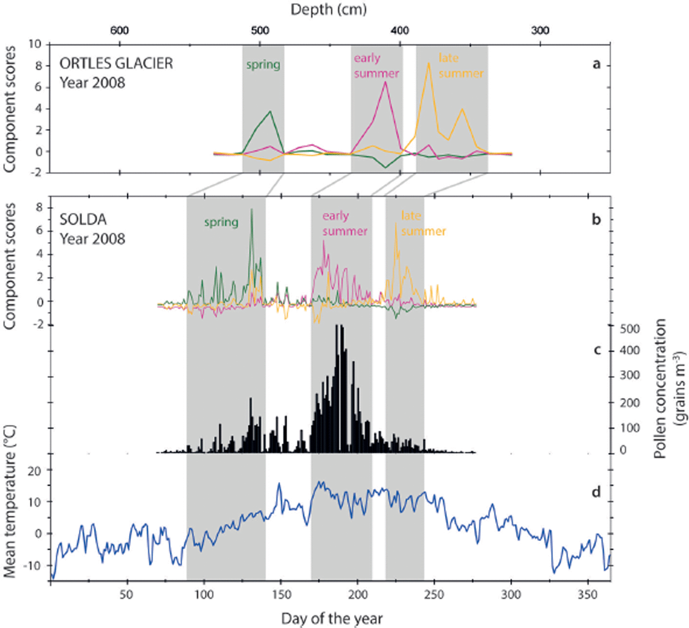
Fig. 5. (a) Principal component scores of pollens for 2008 in the Ortles samples (spring component in green; early-summer component in magenta; late-summer component in yellow). (b) Principal component scores calculated for the daily pollen-monitoring data of Solda in 2008 (PC1: early-summer component in magenta; PC2: spring component in green; PC3: late-summer component in yellow). (c) Total airborne pollen concentration at Solda for 2008. (d) Mean air temperature measured at Solda during 2008.
To better understand factors involved in the timing of pollen deposition on the glacier, Pearson correlation coefficients (see Table 4) have been calculated considering Solda’s PCs, daily airborne concentration at Solda, mean daily temperature and daily precipitation at Solda. Airborne pollen concentration at Solda correlates with mean daily temperature (r = 0.427, p < 0.01). By contrast, daily precipitation does not correlate significantly with the airborne pollen concentration in Solda. As airborne pollen concentration is a result of pollen production and dispersion, the correlations point to the fact that both processes are likely controlled by air temperature and are not very much affected by precipitation. The fact that airborne pollen concentration depends on temperature indirectly supports the use of δD and δ18O as indicators of temperature in the Ortles firn core; Ortles pollen concentration correlates well with the δD and δ18O (see Table 2). In this context it is interesting to observe that, in Solda, correlation coefficients (Table 4) indicate a significant correlation between mean daily temperature and the early- and late-summer components (respectively r = 0.601, p < 0.01 and r = 0.238, p<0.01). In contrast, spring component does not correlate with mean daily temperature. These results are consistent with those obtained for the firn core considering δD and δ18O as temperature proxies: in fact they both correlate with early- and late-summer components (see Table 2) but not with the spring component. Altogether the similarities of the PC pattern and the correlations show a certain consistency in terms of proxy data determined in the Ortles firn and measured data for Solda.
Table 4. Pearson correlation coefficients for Solda daily pollen monitoring and meteorological data for the year 2008. Significant correlations are highlighted in bold (** correlation is significant at p < 0.01; * correlation is significant at p < 0.05)

Conclusions
The results obtained in this study confirm that pollen analyses are a powerful tool for detecting annual and seasonal snow deposition in ice cores. We have demonstrated that an accurate and complete identification and quantification of the pollen content is essential, as complete pollen spectra contain much information about seasonality and enable statistical analyses. The statistical approach presented here is a novel methodology to detect seasonal and yearly changes in the pollen spectra in an objective manner. This method is potentially suitable for longer ice cores, where the use of pollen diagrams characterized by rich pollen spectra and thousands of samples is problematic and makes it difficult to clearly identify patterns. Furthermore, the principal components statistical approach can potentially be applied to other archives where the detection of seasonality in pollen spectra is required, as is the case for cyclic sedimentation (e.g. varved sediments). Finally, the results of our analyses represent an important contribution to the construction of a robust age–depth model for the 10 m Ortles firn core and suggest that pollen analyses on the deeper core will be useful.
Acknowledgements
We thank the Autonome Provinz Bozen – Südtirol, Abteilung Bildungsförderung, Universität und Forschung for financial support to the project PAMOGIS (Pollen Analyses of the Mount Ortles Ice Samples). This work is a contribution to the ‘Ortles project’, a program supported by the Fire Protection and Civil Division of the Autonomous Province of Bolzano, in collaboration with the Forest Division of the Autonomous Province of Bolzano and the Stelvio National Park. This is Ortles project publication No. 5. For collaboration in the various phases of the 2009 field operation we thank Ludwig Noessig, Elmar Wolfsgruber and Claudio Carraro (Ufficio geologia e prove materiali of the Autonomous Province of Bolzano), Marc Zebisch and Philipp Rastner (EURAC), Paul Vallelonga (University of Copenhagen), Michele Lanzinger, Matteo Cattadori and Roberto Filippi (Museo Tridentino di Scienze Naturali) and Silvia Forti (Istituto di Cultura le Marcelline). For logistic support we are grateful to Toni Stocker (Alpine guides of Solda) and the helicopter company Airway. This is BPCRC contribution No. 1537. We thank two anonymous reviewers for useful suggestions.


