


Introduction
In 1973 an ice mass, separated by a large crevasse from the glacier behind, was threatening a village (Randa, Wallis). The time of breaking-off has been predicted quite accurately by extrapolation of the veloci ty- time function measured in the preceding months (Reference FlotronFlotron, 1977; Reference RothlisbergerRothlisberger, 1977). By the same method, the calving of an ice mass from the Grubengletscher (Wallis) was forecast (Reference HaeberliHaeberli, 1975) While velocity measurements are indispensable for such forecasts, a better understanding of the breaking mechanism is desirable. Such a knowledge could improve the choice and layout of future measurements or initiate new investigations. One way of obtaining a better understanding of the process is to set up a model based on existing observations. This has been attempted for the Grubengletscher where the geometry is relatively simple and where both long-term as well as detailed measurements have been made. The glacier borders a shallow lake which undercuts the steep cliff causing calving about once a year. However, the glacier is not floating and buoyancy forces are negligible. The problem thus differs from that of calving from floating ice shelves or ramps which has been treated theoretically by Reference WeertmanWeertman (1957), Reference NyeReeh (1968) and Reference HoldsworthHoldsworth (1973). The mechanism studied in the case of the Grubengletscher applies for an ice mass breaking off from the main ice body under the effect of its own weight. The process starts in the zone of maximum tensile stress which exists at some distance from the cliff as a consequence of the horizontal gradient of longitudinal stress (this stress is equal to the hydrostatic pressure far away from the cliff and zero at the vertical cliff). A crack, starting in the zone of maximum tension does not proceed downwards to the ice edge at once but only in a series of steps each of which corresponds to a greater overhang of the detaching ice mass. This step-wise propagation of a crack is modelled.
Geometry of cliff and results of measurements
In Figure 1 the part of the cliff which broke off in 1974 is sketched; in this paper it will be termed the lamella. The figures refer to an early stage; later the lamella became much thinner by ablation. The movement of the lamella relative to the main glacier has been measured with a kryokinemeter. Observations at intervals of one minute showed that the movement was jerky. Reference Haeberli and RothlisbergerHaeberli and Rothlisberger (1976) assumed that the jerks correspond to the formation of cracks. This suggests the following breaking mechanism:

Fig. 1. Plan (a) and side view (b) of calving front at the Grubengletscher: L = lamella, B = ice block supporting lamella, K = kryokinemeter
Outline of assumed breaking mechanism
The mechanism consists of two alternating processes:
1. formation of a crack which stops at a certain depth;
2. growth of stress at the base of the crack until further crack propagation is possible.
Process I. The crack opens perpendicular to the direction of the tensile principal stress σ1 and stops at a depth where σ1 = 0.
Process 2. Growth of tensile stress at the base of the crack is caused by two further processes:
(a) ice flow which results in an increasing overhang of the lamella;
(b) further undercutting of the cliff by the lake current (neglected in this paper).
It is assumed that, once the crack has stopped, it becomes blunted and therefore a stress cri greater than a critical value σe > 0 is necessary to trigger further propagation.
Assumptions and simplifications
(i) Stresses and velocities are calculated for plane strain, i.e. the lamella sketched in Figure 1b is taken to be of unlimited extent in the direction perpendicular to the paper.
(ii) It is assumed that Glen 's flow law applies for effective stresses > 0.3 bar. In Glen's flow law
(2)
where
are the components of the strain-rate tensor and σij′ those of the stress deviator. τe, the effective stress, is given by 2τe2 = σij' σij′, n is taken to be equal to 3 and A = 580 bar sec1/3 corresponding to the value which Reference NyeNye (1953) obtained from the closure rate of bore holes with a slight modification by Reference RothlisbergerRöthlisberger (1972).(iii) For effective stresses ≤0.3 bar a linear flow law is used. While the choice of the limiting value of 0.3 bar is arbitrary, the adoption of a linear flow law at low stresses is in accordance with results of creep tests by Reference Butkovich and LandauerButkovich and Landauer (1960) and Reference Melior and TestaMelior and Testa (1969). (The latter authors, however, found no strictly linear flow law. Further, they questioned whether secondary creep was established in all creep tests.) In any case, the choice of the flow law for low stresses is of little influence on the calculated velocities.
(iv) It is assumed that the first crack opens in the glacier surface perpendicular to the direction of the tensile principal stress when this stress has grown to a certain value. This critical value is of the order of I bar, as can be inferred from strain-rates measured in regions of glaciers where transverse crevasses form. Reference HoldsworthHoldsworth (1969) reports strain-rates in the range of 0.01 a-1 to 0.0 3 a-1 associated with the formation of transverse crevasses. In our model the tensile stress in the glacier surface grows as the lake current undercuts the cliff deeper and deeper. It is not unreasonable to assume that the first crack forms when the tensile stress in the glacier surface amounts to, say, 0.8 bar which corresponds to an undercut by the lake of 3 m. In any case, the principal process of a step-wise extension of the crack does not depend on this particular assumption. In fact, in a second model of the glacier cliff we have chosen an undercut of 4 m and have in addition introduced the crack closer to the front. The process of detachment was very similar to that in the first model.
(v) The critical tensile stress necessary for further propagation of a crack which had stopped is arbitrarily taken as σc = 0.03 bar.
(vi) The direction of crack propagation is inferred from the stress field calculated at each new onset of crack propagation on the basis of Glen's flow law. Actually, once the crack has started propagating elastic strains determine the direction of further propagation. All elastic effects, however, are neglected. Further deficiencies in the determination of the crack direction are specified in the next section.
(vii) Ablation at the ice surfaces is neglected, although it did significantly change the shape of the lamella at the Grubengletscher
(viii) The effect of water pressure acting on the small submerged part of the lamella is neglected.
Method of computation
Calculations were carried out with a computer program for finite-element analysis of elastic sheets, plates and shells developed by U. Walder and D. Green at the Institut für Baustatik, ETH Zürich. This program is based on a hybrid stress model. The assumed stress field satisfies the equilibrium requirements within an element. Stresses are discontinuous, however, at the element boundaries. Functions for the deformations of element boundaries are chosen in such a way that for equal displacements and rotations in nodal points the deformations of two neighbouring element boundaries are equal. Applying the generalized principle of the minimum of complementary energy the stiffness matrix is calculated. Due to complete analogy of equations, the program can also be used for Newtonian liquids with the flow law:
where η is the viscosity and ![]() are the components of strain-rate deviator. For the special case of incompressibility
are the components of strain-rate deviator. For the special case of incompressibility ![]() can be replaced by
can be replaced by ![]() and then Equation (3) is formally identical with Glen's flow law (2) provided that the term
and then Equation (3) is formally identical with Glen's flow law (2) provided that the term ![]() stands for a stress-dependent viscosity η(τe). Numerical values of η(τe) have been found for each element by means of an iteration scheme: In the first step η was taken to be equal to
stands for a stress-dependent viscosity η(τe). Numerical values of η(τe) have been found for each element by means of an iteration scheme: In the first step η was taken to be equal to ![]() with τ e(1) = 0.3 bar for all elements. With η(2) new values of τ e (different for each element) were calculated: they are called here τ e(2). η(2) was then calculated from the recurrence relations
with τ e(1) = 0.3 bar for all elements. With η(2) new values of τ e (different for each element) were calculated: they are called here τ e(2). η(2) was then calculated from the recurrence relations

and so on. This procedure was continued until two successive values η(i) and η(i+1) did not differ in the first two digits for any element.
Calculations were started with the crack-free cliff (Fig. 2). Mesh points (not shown in Figure 2) at the lower boundary were fixed, because along its edge this glacier is frozen to its bed. Mesh points at the left side of the part considered are fixed with respect to horizontal motion but free to move vertically. (This is appropriate at a very large distance from the front.) In the zone of maximum tensile stress a crack was introduced following the direction of the stress field shown. Once a crack was introduced, the stress field became slightly more inclined below the crack. The crack was deepened in the new direction until the larger principal stress in the element below the crack was no longer positive (tensile). Time ti = 0 was assigned to this stage shown in Figure 3. Figure 3a shows the stress distribution in ice assuming material properties as described above while Figure 3b refers to a Newtonian liquid. Note the greater depth of the crack and the much larger tensile stresses in the interior of the lamella of Figure 3a as opposed to Figure 3b. The latter peculiarity is a consequence of the lower stress-dependent viscosity at the base of the lamella. This will be considered in the next section.

Fig. 2. Model of ice cliff undercut by shallow lake at the right-hand edge. Numbers are values of the more-tensile principal stress σ, in tenths of bar, upright numbers indicate tension, slanting numbers compression. The dotted line is the boundary between tensile and compressive values of σ1. Line elements indicate direction perpendicular to σ1. Below the arrow a crack will be introduced.

Fig. 3. a. Same cliff as Figure 2 with stable crack (i.e. stress below crack tip is compressive).
b. Same cliff as Figure 2 with stable crack, material is a Newtonian liquid. (The material shown in all other figures obeys Glen's flow law for effective stresses > 0.3 bar.)
From the calculated velocities of the mesh points at the surface of the lamella, movements over a chosen small time increment Δt were inferred. Drawing these displacements the next position of the lamella was found and the time t 1 = t 1+Δt 1 was assigned to it. Figure 4 shows the lamella after three such steps, at time t 4. In Figure 4a the crack is unstable because σ1 > 0 at its tip. It is extended until σ1 in the element below the crack is no longer positive (Fig. 4b). At depths greater than, say, 17 m the direction of further crack propagation becomes difficult to infer. The reason is that then the principal stress σ2 is so large that immediately below the crack it is necessarily parallel to the traction-free crack surface the shape of which is determined by the quadrilateral finite elements. Simply by continuity the crack has then been extended smoothly towards the edge of the cliff. A stage of this procedure is shown in Figure 5. In the surface of the inner side of the curved crack, tensile stresses have developed parallel to the crack surface. Quite possibly the true crack then follows a zig-zag path. Detailed examinations of the crack path are outside the scope of this study.

Fig. 4. a. Later stage with overhanging lamella. Crack is unstable (i .e. stress below crack tip is tensile).
b. Same overhang of lamella as in Figure 4a. Crack is deeper and stable.

Fig. 5. Distribution of both. principal stresses in overhanging lamella. Small numbers are values of principal stress σ, in tenths of bar, always compressive. Larger, thinner numbers are values of σl (straight numbers indicate tension, slanting numbers compression). Line elements indicate direction of σ. The dotted line is the boundary between tensile and compressive values of σl. Inside the broken line the effective stress is greater than 0.65 bar.
Discussion of stress distribution. Preferred fracture zones
In Figure 5, numerical values of σ2 are shown beside those of σ1. At first sight the absolute values of σ2 next to the upper surface of the lamella appear surprisingly large. The reason becomes clear when the distribution of effective stress is inspected: The effective stress ![]() ) is largest in the lower core of the lamella; inside the broken line —·—·— it is greater than 0.65 bar resulting in a relatively low viscosity
) is largest in the lower core of the lamella; inside the broken line —·—·— it is greater than 0.65 bar resulting in a relatively low viscosity ![]() . The stiffer frame outside the broken line is bending, partly due to its own weight, partly due to the pressure acting from the inside on the curved side-walls of the frame. While the angles at the upper corners of the frame remain nearly unchanged, the side-walls bend outwards and the upper surface inwards. This explains why large compressive stresses occur parallel to the upper surface of the lamella and why large tensile stresses are formed at greater depth (below the “neutral zone” of the “top beam“). The curvature of the frame also explains why tensile stresses occur in the frame adjacent to the crack.
. The stiffer frame outside the broken line is bending, partly due to its own weight, partly due to the pressure acting from the inside on the curved side-walls of the frame. While the angles at the upper corners of the frame remain nearly unchanged, the side-walls bend outwards and the upper surface inwards. This explains why large compressive stresses occur parallel to the upper surface of the lamella and why large tensile stresses are formed at greater depth (below the “neutral zone” of the “top beam“). The curvature of the frame also explains why tensile stresses occur in the frame adjacent to the crack.
The lateral tensile stresses in the upper part of the core of the lamella increase with time during the process of detachment. In the stage shown in Figure 6 they already exceed the stress at which the first crack in the glacier surface opened (Fig. 2), provided that air has access to the interior of the lamella. It is thus possible that the lamella breaks apart along a surface approximately through its centre and parallel to the ice front- and this considerably earlier than the event of detachment of the whole lamella which would be predicted from velocity measurements. Indeed, this kind of failure seems to have taken place in a relatively thick lamella breaking off from the Grubengletscher in 1975 (personal communication from W. Haeberli). Typically, at the surface of the lamella no crack appeared prior to the moment of break-off (as shown in Figure 5, lateral stresses are compressive in the upper surface). The difference in failure of the two lamellae has its correspondence in the calculations which show that towards the end stage the tensile stresses in the core of a thick lamella become larger than those in a thin lamella of the same height.

Fig. 6. Lamella shortly bifore breaking-off, the broken line shows a possible surface of shear fracture.
Another probable fracture zone is the lower edge of the ice front facing the lake. In 1974 from this zone of the lamella an ice mass detached three hours before the entire lamella broke off (Reference HaeberliHaeberli, 1975).
Shear fracturing might also be expected, although it has not been observed at the Grubengletscher. On the basis of Haynes’ interpretation of his triaxiallaboratory tests on strength of ice (Reference HaynesHaynes, 1973), one would expect shear fracture along planes making angles of approximately 30° with the direction of σ2. Such a surface is sketched in Figure 6 (dashed line). It is questionable, however, whether this particular result applies for glaciers, because the strength values from laboratory tests are generally an order of magnitude larger than those at which fracture in glaciers actually takes place.
Velocity of lamella as function of time
Velocities v of the mid-point of the upper boundary of the lamella relative to the m ain glacier were calculated for different stages of inclination of the lamella and stable crack. Time intervals between two successive stages i and i+1 were calculated from the movement between these stages (a) by assuming constant initial velocity vi during the time interval (this method was mentioned under “procedure of calculation“), (b) from the relation
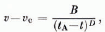
where ti is the time at stage i, di the distance moved between stages i and i+1, vi the velocity at stage i, and vi the velocity at the mid-point of the time interval inferred from an approximate velocity-time function (I). Suitable constants v c and t A were then chosen and the differences v i—v c and t A—ti were plotted on double-logarithmic paper (Fig. 7). A straight line was drawn through these points, representing a function of the form (1). In Figure 7 two modelled and two measured velocity- time functions are shown together : Points I, 4, 6, and 9 of line III correspond to the different stages of the modelled lamella shown in Figures 3a, 4b, 5 (with longer crack) and 6. Time intervals were calculated with method (b).
The points of line IV correspond to a model of a thinner lamella which is more similar to the one measured in 1974. The height of the cliff in this model is 20 m, the distance of the crack from the ice front I1 m and the horizontal extent of the undercut is 4 m. Time intervals were calculated with method (a), the first interval in two steps with the aid of an interpolated point.
The points of lines I and 11 were obtained from the measurements made at the two lamellae detaching from the Grubengletscher in the years 1974 and 1975 respectively.
At time t = tA the velocity becomes infinite according to Equation (1); this implies that the actual detachment takes place at a time R ≤ tA. In the models R is assumed to be close to the time when the centre of gravity of the lamella moves past the supporting edge of the bed (where it borders the lake). For the lamellae measured at the Grubengletscher the time R of final collapse is known; when fitting Equation (I) to the data, t A turned out to be only one minute later than R.
Figure 7 shows that both measured and modelled data are reasonably well described by Equation (I). In view of the complex geometry and support conditions of the lamella measured in 1974 a better agreement with results can hardly be expected.

Fig. 7. Velocity v of lamella as function of time t.
Line I: Velocities measured at the Grubengletscher in 1974 (vc = 0 mm/h, tA = 1000 h). Line II: Velocities measured at the Grubengletscher in 1975 (vc = 0 mm/h, tA = 1000 h). Line III : Modelled velocities, lamella is shown in Figures 3a, 4a–6 (vc = 0.03 mm/h, tA = 18018 h). Line IV: Modelled velocities of thinner lamella (dimensions given in the text) (vc = 0.03 mm/h, tA = 17640 h).
The effect of choosing a different value for A in Glen's flow law (2) would be equivalent to a translation of all modelled points in Figure 7 in the direction making an angle of 1350 with the abscissa.
Changing the size (not the shape) of a lamella has a similar effect: The points of a lamella enlarged by a factor ƛ would have a λ4times higher velocity. The path of a point between two stages of the lamella would be λ-times greater than before, thus the time interval between the stages would be reduced by a factor λ3. In the graph this corresponds to a shift of all points by 3 log λ along the abscissa (towards the left) and 4 log λ along the ordinate. An interesting aspect of practical importance is that the time interval between tA (time of asymptote) and R (time of actual break-off) is reduced by a factor λ3 while the velocity at break-off is enlarged by a factor λ4.
Conclusions
Comparing the velocity-time function of the measured three-dimensional lamella (I) with those of the two-dimensional models, of course no quantitative coincidence is found. However, the type of function is the same in both cases. This is taken as corroboration of the basic assumptions of the model.
Unless shape and material properties of the detaching ice mass were known in detail and a three-dimensional model constructed, no quantitative predictions would be possible. What knowledge, then, may be gained from an approximate two-dimensional model?
I. Zones of large tensile stresses in the interior of a lamella can be detected. There, the magnitude of the tensile stresses is a measure of the probability that failure occurs in these zones before the whole lamella breaks off (and before the predicted time of this event).
2. The approximate deformation of the ice mass can be calculated. This permits one to distinguish whether an observed shape change is the result of normal ice flow or whether it is due to fracture or possibly enhanced flow going along with a change of ice properties in certain zones.
3. Approximate rules for the influence of size and shape of the detaching ice mass on the velocity can be worked out.
Acknowledgements
I wish to thank Dr W. Haeberli, Dr K. Hutter and Dr H. Röthlisberger for several stimulating discussions, for valuable advice, and for the encouragement to carry out this study. Dr Hutter also read the manuscript carefully and suggested many improvements.
The computation was done with a finite-element program for analysis of elastic sheets, plates and shells developed by U. Walder and Dr D. Green at the Institut für Baustatik, ETH Zürich. I am indebted to U. Walder, who advised on the choice and use of the program and to H. jensen, who advised on problems of programming and who fitted curves to the velocity data.
A great part of the work at the computer centre was carried out by L. Papp whose help is gratefully acknowledged.
Discussion
R. List: Your mathematical model is not continuous whereas the equation for the velocity is. What is the time interval between cracks in the model? How does it affect the result and how does it compare with the cracking in nature?
A. Iken: The function inferred from the calculated points is continuous only on a large scale. In the model, the time intervals are calculated from the velocity of the ice flow alone. The time involved in actually propagating the cracks is neglected. The observed time intervals between cracks were small; Reference HaeberliHaeberli (1975) observed several cracks per minute.
H. Röthlisberger: In spite of the generally very regular acceleration there were short-term irregularities in the case of the small glacier of the Weisshorn above Randa, which could not be explained by surveyors' error. This may indicate that the ice mass moves with discrete jerks.
J. W. Glen: Why did you not allow for any increase in the overhang due to undercutting by the water?
I Ken: The erosion by lake water was neglected because
(I) It has not been measured.
(2) We think that the effect of progressive ice erosion on the breaking process is small compared to that of ice flow once the breaking process has started.
D. M. McClung: Can you comment on how you are able to model the stresses at a crack tip and the propagation of a crack with a viscous flow law?
Iken: I did not model the crack propagation itself but calculated the stresses before and after each propagation. I did not calculate the stress concentration at the tip. However as soon as the more tensile of the principal stresses, σ1 is zero or compressive at some distance from the tip, the crack cannot propagate further, no matter what the crack tip looks like.


