


1. Introduction and Background
The subject of this paper is ice from Vostok core 5G, which was obtained at the Russian Vostok station in East Antarctica (78°28’S, 106°48’ E) through collaboration between Russia, France, and the United States. The coring reached a depth of 3623 m in January 1998. The altitude is 3488 m a.s.l., the present-day mean air temperature at the surface is –55.5°C and the annual accumulation is 2.2–2.5 gcm–2 (Reference JouzelJouzel and others, 1987; Reference Lipenkov, Barkov, Duval and PimientaLipenkov and others, 1989; Reference Salamatin, Vostretsov, Petit, Lipenkov and BarkovSalamatin and others, 1998).
The Vostok core is important because it contains ice formed under unique circumstances. It differs from other cores, even in Antarctica, due to the cold, dry local climate, the distance from the divide (120 km), and a low surface slope (1 × 10⁻³mm–1) but with a significant (3ma–1) horizontal flow. For example, it is estimated that at 2083 m, where the temperature is –36°C, the vertical strain rate is 7 × 10⁻⁶ a–1, the horizontal shear stress at 2000 m is <20 kPa and the shear strain rate is approximately 4 x 10⁻⁶a–1(Reference Lipenkov, Barkov, Duval and PimientaLipenkov and others, 1989; Reference Salamatin, Vostretsov, Petit, Lipenkov and BarkovSalamatin and others, 1998). The fabric and texture of the initial 2083 m of the core is described in Reference Lipenkov, Barkov, Duval and PimientaLipenkov and others (1989). The authors found that the crystal growth rate is lower during the cold periods, identified from the oxygen isotope δ18O record as 13– 30kyrBP (about 300–500m) and 140–160 kyr BP (about 1900–2083 m), than in warm periods that include the past 13 kyr BP(shallower than 300 m) and 116–140 kyr BP (1600– 1900 m). They also noted that crystal shape becomes elongated in a horizontal direction below 100 m, changing most between 350 and 500 m. Crystal orientation is initially quasi-uniformly distributed, but beginning at about 454m assumes a vertical-girdle nature where the direction of grain elongation is nearly orthogonal to the vertical plane containing the c axes. This is important because it demonstrates that the ice at this location is deformed both from basal glide brought on by compression and from horizontal tension. The vertical-girdle fabric persists in the remainder of their pole figure to 2083 m, i.e. the fabric does not vary with temperature (δ18O) (Reference Lipenkov, Barkov, Duval and PimientaLipenkov and others, 1989).
Dating and paleoclimatic interpretations of the isotopic record in the deep borehole (below 1800 m) were presented by Reference Salamatin, Vostretsov, Petit, Lipenkov and BarkovSalamatin and others (1998), the result of a comparison and reconciliation of data from four different temperature profile analyses conducted between 1988 and 1998.
Grain-size, deuterium profile and seismic wave-speed measurements for the deeper parts of the core were presented by Lipenkov and Barkov at an international workshop in St Petersburg in 1998 (Reference Lipenkov and BarkovLipenkov and Barkov, 1998). The figure from their abstract, reproduced as Figure 1 without change to the figure or caption, describes an internal structure characterized by zones of markedly different texture and fabric, beginning most noticeably at 2700 m. Two distinct microstructures, categorized as A and B zones, alternate. A-type zones, which include, but are not strictly limited to, warmer interglacial periods, are characterized by larger grains with a vertical-girdle orientation, i.e. their caxes fall in a plane encompassing the vertical. The vertical-girdle fabric arises from the rotation of grains by basal glide under conditions of vertical compression coupled with uniaxial tension in the direction of flow (Reference Lipenkov, Barkov, Duval and PimientaLipenkov and others, 1989; Reference PatersonPaterson, 1991). Reference Castelnau, Canova, Lebensohn and DuvalCastelnau and others (1997) developed a model that assumes uniform stress and strain within each grain of ice, and deformation primarily by basal slip. When De La Chappelle and others (1998) applied this visco-plastic self-consistent (VPSC) model to simulate the development of the vertical-girdle fabric at Vostok, it produced a far tighter girdle than is actually found there. They attributed this difference to polygonization. In nature, grains with c axes already parallel to the direction of compression cannot deform by basal glide: axial stresses parallel and perpendicular to the c axis grow and bending moments appear. This leads to competition between lattice rotation by basal slip and polygonization. Polygonization is defined as the process whereby further strain, after a strong preferred fabric has developed, causes the alignment of dislocations within grains and the subsequent formation of sub-grain boundaries and additional new grains that differ in orientation from the c axis of the original grain by only a few degrees.
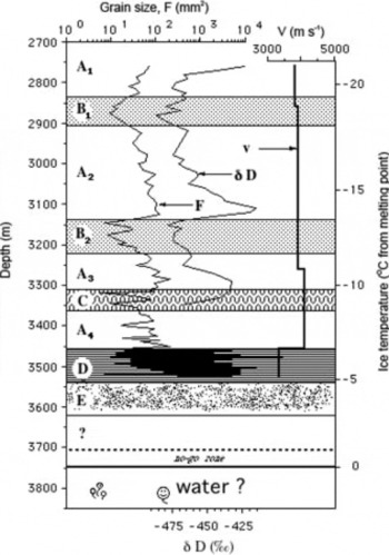
Fig. 1. Internal structure of the Antarctic ice sheet at Vostok station (2700-3623 mbs) (Reference Lipenkov and BarkovLipenkov and Barkov, 1998). Reprinted with permission of the authors. A1–4 Zones of relatively coarse-grained ice with girdle-type fabric corresponding to uniaxial extension of ice along flow line; B1,2 Zones of relatively fine-grained ice with single-maximum fabric corresponding to shear; zones B coincide with the ice strata formed under conditions of glacial maxima (high impurity concentration); C Former zone of ice-flow disturbance (?); D Layered ice stratum interpreted as a sole of the moving section of the ice sheet; E Basal ultra-coarse-grained silty ice considered as stagnant ice. Remarkable correlation between the grain-size (F, mm2) and the deuterium profile (δD,%) (Reference PetitPetit and others, 1998) indicates the link between the internal structure of the ice sheet and climate. Vertical profile of seismic wave speed (ν, m/s) (Reference Popkov, Verkulich, Masolov and LukinPopkov and others, 1999) exhibits significant decrease in ν within stratum D.
In contrast, B-type zones, which coincide with cold conditions and glacial maxima (Reference Lipenkov, Barkov, Duval and PimientaLipenkov and others, 1989; Reference Lipenkov and BarkovLipenkov and Barkov, 1998; personal communication from V. Lipenkov, 2005), have higher impurity concentrations, smaller average grain sizes and a single-maximum fabric. A single-maximum fabric is usually produced by vertical compression (and divergent horizontal tension) (Reference Azuma and HigashiAzuma and Higashi, 1985) or by simple shear near the base of a glacier (Reference Budd and JackaBudd and Jacka, 1989). The authors noted that these different fabrics (single maximum and vertical girdle) are characteristic of different stress conditions, and suggested that their interpretation requires an assumption of discontinuity in the recrystallization and deformation processes that may be attributed to structural softening.
After the first two alternating A and B zones, the third interglacial zone, A3, is followed by a zone labelled C (3310–3370m) (see Fig. 1), which contains evidence of stratigraphic disturbance. At 3311 m, there are three ash layers a few centimeters apart but sloping in opposite directions (Reference PetitPetit and others, 1999). At 3321 m, there is a shift in deuterium content from interglacial-like to glacial-like conditions and then back again, accompanied by a transition in CO2 and CH4 gas levels from glacial-like (low) to interglacial-like (high) conditions (Reference PetitPetit and others, 1999). The gas transition associated with a change from glacial to interglacial conditions would normally be expected somewhat deeper (~10 m) (Reference PetitPetit and others, 1999). These features have led some to conclude that the C zone has undergone folding (Reference PetitPetit and others, 1999; Reference SimôesSimões and others, 2002). Interestingly, it was concluded that deeper ice (3370–3538 m) was undisturbed, based on the lack of structural incongruities and the observation that air hydrate crystals there exhibited uninterrupted growth with depth (Simões and others, 2002). A fourth A-type zone, A4 (Fig. 1), found from 3370 to 3460 m, is followed by zone D (3460-3538 m), the main shear layer of the moving ice sheet, which is characterized by rapidly alternating A- and B-type layers. At the bottom of the meteoric ice lies zone E (3538-3605 m), which consists of very coarse-grained silty basal ice. The last 17 m of the core are accretion ice, formed by melting and refreezing as the glacier passes over Vostok Subglacial Lake. Drilling ceased at 3623 m, approximately 100m above the subglacial lake.
Early attempts to date the Vostok core using gas isotope data (Reference PetitPetit and others, 1999) ended at 3310 m because of the discontinuity in the climate record noted at 3311 m. Between 3320 and 3330 m an abrupt transition from interglacial to glacial deuterium (δD, a proxy for local temperature) and gas (CO2 and CH4) content, and then back to interglacial values, was observed. Nonetheless, recent efforts have produced dating for depths below 3350 m (Reference Salamatin, Tsyganova, Lipenkov and PetitSalamatin and others, 2004). The latter approach applies three different techniques for dating: (i) the geophysical metronome timescale (GMTS);(ii) correlation of the Vostok ice-core deuterium–depth signal with a second independent oxygen-isotope (δ18O) based timescale (DHVTS, from the calcite core (DH-11) in Devils Hole, NV, USA);and (iii) ice- flow modeling fitted to both the GMTS and DHVTS. Despite the stratigraphic disturbance reported at 3311 m (Reference PetitPetit and others, 1999), Simdes and others (2002) have shown that glacial stages 14 and 16 are still distinctly discerned in the dust concentration record within the depth intervals 3393–3405 m and 3440–3455 m, respectively, and evidence of interglacial stage 17 appears from 3457 to 3466 m. This suggests that strata as deep as 3466 m have undergone only local perturbations. Reference Salamatin, Tsyganova, Lipenkov and PetitSalamatin and others (2004) use their constrained ice-sheet flow model to extrapolate the mean ice age–depth curve to produce theoretical dating for the rest of the Vostok meteoric ice. This provides the depth–age scale we use in this paper.
This paper presents the microstructure and impurity content of a number of specimens ranging in depth from 97 to 3416 m, describes in detail the characteristics of different layers and proposes a mechanism for the development of these layers.
2. Measurement Methods
The Vostok 5G core specimens used in this study were stored at –35°C for 7 years at the US National Ice Core Laboratory
(NICL) in Denver, CO, and later at –25°C for 1 year in the Ice Research Laboratory (IRL) at the Thayer School of Engineering at Dartmouth College. The depths of the sections used for this study are shown in Table 1. These depths are from the bags of specimens retrieved from storage at NICL and shipped there from Vostok station. Depth data for a few sections are available only to the nearest meter. Herein, the section depths will be referred to by integer numbers except where greater specificity is useful and available.
Table 1. Textural data for all Vostok samples, including the number of grains measured

2.1. Grain size
Vertical thin sections were prepared for grain-size measurement. Grain size (area) was measured using two different methods. First, we used the standard linear intercept method (Reference Alley and WoodsAlley and Woods, 1996; Reference GowGow and others, 1997) (200 intercepts obtained for each depth). Second, we used the pixel-counting area measurement utility of an image-processing application, Image SXM (W.S. Rasband, http://rsb.info.nih.gov/ij;S.D. Barrett, http://www.liv.ac.uk/~-sdb/ImageSXM). For larger-grained specimens, multiple thin sections were analyzed with Image SXM so that at least 100 grains were measured for each depth, and over 600 grains for each specimen from <1200 m. The two methods yielded results that were within 7–28% of one another, but for accuracy and consistency, the pixel-counting data are used for the grain area reported (Table 1). Linear intercept data were used to calculate flattening, where aspect ratio is the average grain width divided by the average grain height.
2.2. Ion chromatography
A Dionex DX-120 ion chromatograph with Dionex IonPac AG14 + AS14 anion columns and CG12A + CS12A cation columns was used to gather ion concentration data in our samples. The flow rate was 1.6mLmin–1 and the pressure was approximately 11.86 MPa. The eluent was 3.5 mmol L–1sodium carbonate/1.0 mmol L–1 sodium bicarbonate. The instrument detection limits (IDL) for anions were 5–20 ppb Cl–, 20–30 ppb NO3 – and 20–40 ppb SO4 2¯ For cations, the IDL were 1 ppb Na+, 1 ppb NH4+, 2 ppb K+, 8 ppb Mg2+ and 15 ppb Ca+. The instrument was calibrated using a quadratic fit of six standards with the calibration curve forced through zero. Calibration verification samples were run at the middle and end of each run. Midway through the cation run, it was found that the instrument had drifted upward such that it biased the results 20% high. The order of samples run through the cation column was 2874, 3399, 3329, 2749, 3311, 3321, 399, 1849 and 650 m, and the calibration sample was run after the specimen from 2749 m.
The chromatograph required 5mL of each sample for each run. This was obtained by cutting a piece of the specimen that was approximately 1.5 cm x 2.0 cm × 2.0 cm with a small bandsaw, then shaving the six sides of the piece with a razor blade under a HEPA (High Efficiency Particle Air)-filtered laminar-flow hood, handling the sample only with tweezers and a spatula. All tools used during specimen preparation were carefully pre-cleaned using acetone, methanol, n-hexane and deionized water.
Samples were melted in clean plastic sample bottles and were tested using the anion column. Repeatability was assessed by additional testing conducted later on separate samples from some depths. The cation column was acquired more recently and, due to time and limited sample availability, only certain core depths were tested and only one test was run on each.
2.3. Scanning electron microscopy/energy-dispersive spectroscopy
Our technique for scanning electron microscopy (SEM) and energy-dispersive spectroscopy (EDS) of uncoated ice has already been described in detail (Reference Cullen and BakerCullen and Baker, 2000, Reference Cullen and Baker2001; Reference Baker, Cullen and IliescuBaker and others, 2003). Samples approximately 2.5 cm × 2.5 cm × 1.0 cm were cut and their surfaces were shaved flat with a razor blade. The sample was frozen onto a brass plate and placed in a sealed container at –25°C for approximately 24 hours. While in the scanning electron microscope, the samples were held at –85 ± 5°C.
2.4. Electron backscatter diffraction
Uncoated ice specimens were prepared and subsequently examined in an FEI XL-30 environmental scanning electron microscope using the electron backscatter diffraction (EBSD) technique described in detail by Reference Iliescu, Baker and ChangIliescu and others (2004) and Reference Obbard, Baker and SiegObbard and others (2006b). Specimens with dimensions of approximately 3.0cm × 1.5 cm × 3.0 mm were cut from core specimens such that the specimen surface lay perpendicular to the core axis. Multiple samples from the specimen were cut with the same orientation (i.e. with their long sides parallel) so that orientation data from multiple pieces of the same specimen could be plotted on a single pole figure. Other than this, there is no way of knowing the azimuthal orientation of the specimen, and differences in the direction of a vertical-girdle pattern on a pole figure are not significant.
Approximately 100 grains were measured in each sample. The measurement of more grains would have been desirable (200 is typical), but we were limited by the size of available Vostok specimens and the competing sample requirements of other analyses (e.g. ion chromatography).
Grain boundaries and triple junctions were identified visually on the specimen using the SEM imaging capabilities. Grain boundaries were identified by a clear grainboundary groove and/or a change in the surface etching pattern, the pattern of white spots on a black background that varies with lattice orientation (Reference Obbard, Baker and IliescuObbard and others, 2006a). For each grain, a representative EBSD pattern was collected. The implied change in specimen orientation due to moving the beam across the specimen is 1.07° per 2 mm traverse on the specimen, which is consistent with the typical ~1° ‘orientation noise’ reported by Reference Bate, Knutsen, Brough and HumphreysBate and others (2005). Typically, the distance between measurements was ≤500μm. Hence, misorientations between adjacent grains were determined to an accuracy of ~0.5°.
The EBSD patterns were indexed with HKL Technology’s CHANNEL ![]() software. The misorientation between grains is described using the angle and axis for the smallest possible rotation that can be applied to one grain to achieve lattice coincidence with the other. Misorientation angle and axis were calculated from crystal orientation using the CHANNEL
software. The misorientation between grains is described using the angle and axis for the smallest possible rotation that can be applied to one grain to achieve lattice coincidence with the other. Misorientation angle and axis were calculated from crystal orientation using the CHANNEL ![]() software according to the method of Reference Randle and EnglerRandle and Engler (2000). The distribution of misorientation angles between adjacent grains (i.e. correlated misorientations) is compared with the theoretical distribution of misorientation angles between randomly oriented hexagonal grains and the distribution of misorientation angles between each grain pairing in the sample (uncorrelated misorientations). An uncorrelated distribution that differs from the theoretical random indicates a preferred orientation throughout the material (fabric). A non-random distribution of correlated misorientations suggests a special relationship between some adjacent grains such as that found with twinning.
software according to the method of Reference Randle and EnglerRandle and Engler (2000). The distribution of misorientation angles between adjacent grains (i.e. correlated misorientations) is compared with the theoretical distribution of misorientation angles between randomly oriented hexagonal grains and the distribution of misorientation angles between each grain pairing in the sample (uncorrelated misorientations). An uncorrelated distribution that differs from the theoretical random indicates a preferred orientation throughout the material (fabric). A non-random distribution of correlated misorientations suggests a special relationship between some adjacent grains such as that found with twinning.
3. Results
3.1. Texture
Thin sections and average grain area for representative shallow specimens and all specimens from a depth of over 2700 m are shown in Figure 2. Texture data for all sections are shown in Table 1. Grain size (area) generally increases with age, with a few notable exceptions, as shown in Figure 3. We calculated the age of the core at each depth using the data presented by Reference Salamatin, Tsyganova, Lipenkov and PetitSalamatin and others (2004) and linear interpolation between ages of adjacent depths (personal communication from V. Lipenkov, 2005). The ages determined for the samples from the A4 zone (494 506 years BP at 3399.68 m and 519491 years BP at 3416.55 m) are for plotting purposes only, as the stratigraphic disturbance in zone C, discussed earlier, makes dating for these layers uncertain. A linear fit of the data from 97 to 2749 m and 3300, 3311 and 3329 m is represented by:
where t is time in years. Exceptions to the linearly increasing grain area with age are found at 2874, 3321 and 3399 m, where the grain size is quite a bit smaller than would be expected. The 3321.765–3321.805 m specimen not only has an average grain size of 8.83 mm2, which is quite low, but in this case a simple average is misleading because in a thin section (Fig. 2) we see horizontal zones of significantly different grain size. Grain size is plotted as a function of depth for this thin section (representative of other sections made from this specimen) in Figure 4. Note that even the largest grains are much smaller than those that would fit Equation (1) (61.167 mm2). Note also that the grains in the coarser-grained layer are more equiaxed than those above or below.
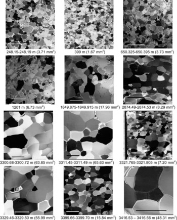
Fig. 2. Vertical thin sections (scale bars 10 mm). Grain area was determined from multiple thin sections using pixel counting.

Fig. 3. Mean grain area for Vostok 5G as a function of age (determined using Reference Salamatin, Tsyganova, Lipenkov and PetitSalamatin and others, 2004) and linear fit derived as described in the text. Starred points are those identified as belonging to B-layers.
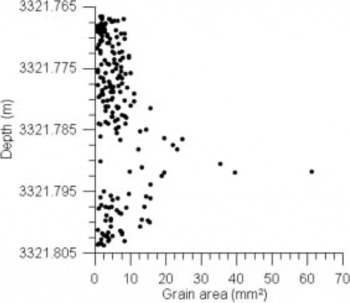
Fig. 4. Variation in grain area with depth for vertical thin section from 3321.765 to 3321.805 m. The x axis is grain area, which is determined by pixel counting and plotted at the depth of the center of mass of each grain.
Grain flattening was observed, and therefore measured, in the deeper sections and is quantified by an aspect ratio (grain width:grain height) <1 (see Table 1). In the 2874, 3321 and 3399 m specimens, not only was grain size unusually small compared with that in the other layers and with that expected from the curve represented by Equation (1), but grains were also more significantly flattened than in other layers, another sign of reduced grain growth. Aside from this vertical thinning, there were no other changes in grain shape with depth. Lipenkov and others (Reference Lipenkov, Barkov, Duval and Pimienta1989, fig. 1) show that below 100 m, grains elongate in one horizontal direction. Horizontal thin sections prepared from both our interglacial and glacial specimens did not reveal this (two horizontal thin sections are shown in Fig. 5).

Fig. 5. Horizontal thin sections from (a) 3399 m and (b) 3416 m in the Vostok core showing no apparent difference in grain width in a horizontal direction. Sections are approximately 4 cm wide on the flat sides.
3.2. Fabric
The {0001} and ![]() pole figures for each specimen depth are shown in Figure 6. Note that each hexagonal crystal supplies one pole on the {0001} pole figure, but three, 60° apart, on the
pole figures for each specimen depth are shown in Figure 6. Note that each hexagonal crystal supplies one pole on the {0001} pole figure, but three, 60° apart, on the ![]() pole figure. In Figure 6, we see a random distribution of poles in the 97 and 248 m specimens. The pronounced vertical girdle is first noted at 1201 m, and then in eight out of the remaining eleven specimens, where it strengthens with depth. A singlemaximum fabric is observed in the deeper layers that are associated with the glacial periods, as reported by Reference Lipenkov, Barkov, Duval and PimientaLipenkov and others (1989). The deeper layers possessing a single maximum (2874, 3321 and 3399 m) correspond with those with abnormally small grain sizes and greater flattening. In the {0001} pole figures from depths of 1500 m and greater, there are some clusters of poles. These indicate grains having similar c axis orientations, and suggest a preferred orientation or fabric. However, the clusters alone do not tell us anything about the relative location of these grains in the specimens. For those depths also characterized by many low-angle (1–10°) misorientations between correlated (adjacent) grain pairs, these clusters may be indicative of polygonization. This possibility is addressed in section 4, and a more in-depth examination of the theory behind it can be found in Reference Obbard, Baker and SiegObbard and others (2006b).
pole figure. In Figure 6, we see a random distribution of poles in the 97 and 248 m specimens. The pronounced vertical girdle is first noted at 1201 m, and then in eight out of the remaining eleven specimens, where it strengthens with depth. A singlemaximum fabric is observed in the deeper layers that are associated with the glacial periods, as reported by Reference Lipenkov, Barkov, Duval and PimientaLipenkov and others (1989). The deeper layers possessing a single maximum (2874, 3321 and 3399 m) correspond with those with abnormally small grain sizes and greater flattening. In the {0001} pole figures from depths of 1500 m and greater, there are some clusters of poles. These indicate grains having similar c axis orientations, and suggest a preferred orientation or fabric. However, the clusters alone do not tell us anything about the relative location of these grains in the specimens. For those depths also characterized by many low-angle (1–10°) misorientations between correlated (adjacent) grain pairs, these clusters may be indicative of polygonization. This possibility is addressed in section 4, and a more in-depth examination of the theory behind it can be found in Reference Obbard, Baker and SiegObbard and others (2006b).

Fig. 6. Fabric diagrams and misorientation histograms for Vostok 5G sections. Plotted points are projections onto the equal-area net, of each crystal orientation intersection with the upper hemisphere. n is the number of grains measured.

Fig. 6. continued.

Fig. 6. continued.
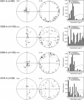
Fig. 6. continued.
The distribution of correlated misorientation angles for each depth is also shown in Figure 6, along with the random (theoretical) distribution curve (solid line) and the distribution of uncorrelated misorientation angles (dashed line). The calculated misorientations are binned into 5° groups, so the vertical axis must be multiplied by five for the groups to sum to unity. At 97 and 248 m, where the fabric is randomly oriented, the misorientation angle distribution, both correlated and uncorrelated, is also reasonably random. The vertical-girdle fabric seen in pole figures for many of the deeper specimens is manifested in the non-random nature of the uncorrelated misorientation distribution. The correlated misorientations for these specimens are more heavily weighted toward the low (0–10°) angles than the overall (uncorrelated) mis- orientation (fabric). In the specimens with a strong singlemaximum fabric, both the uncorrelated and correlated misorientations are predominantly <40°. This is additional evidence of the strong fabric in these specimens, and of the lack of special relationships between adjacent grains.
3.3. Impurity content
Impurity content is shown in Table 2. Soluble impurities are those soluble in the 25°C meltwater and hence measured with ion chromatography. Dust levels were measured with laser light scattering through the solid, and thus would include the soluble portion, if any, of particulates. Hence we call dust (and ash) particulates rather than insoluble impurities.
Table 2. Impurity concentration in mass ppb

3.3.1. Soluble impurities
Variations in concentrations of specific ions over the two or three runs can be seen and may be due to the location in the specimen from which the sample was cut. Initial samples were cut horizontally from the bottom of the specimens. Thus, the first anion concentration value shown for each depth is not necessarily representative of the whole 3–4 cm thick specimen. Second and third anion samples and all cation samples were cut vertically from the specimens and so tend to yield average concentrations over a depth of 3–4 cm. To assess the repeatability of the test set-up, back-to- back cation runs from the same bottle of melt were carried out for 3311m and were within 2 ppb for each cation measured (hence only one of these values is shown in Table 2). However, the first two sets of anion analysis of the 3311 m specimen shown in Table 2 were run on successive days from different bottles of melt (which came from different pieces of the specimen) and are not within the anion IDL, e.g. Cl– concentration was 135 ppb on the first day and 220 ppb on the second day compared with an IDL of 20 ppb. Thus, samples made from pieces cut vertically from 3–4 cm of core are unlikely to yield the same results each time or to be representative of smaller layers within the specimen, such as those found at 3321 m. Results from continuous ion chromatography would provide more precise ion concentration data, but are not available for part of the core examined in detail herein (Reference Legrand, Lorius, Barkov and PetrovLegrand and others, 1988).
3.3.2. Particulates
The dust concentration data included in Table 2 were compiled from Reference PetitPetit and others (1999) and Reference SimôesSimões and others (2002) by V. Lipenkov (personal communication, 2004) and include values from both the 3G and 5G cores at Vostok station, as indicated. These data were not collected continuously for the core and are available only at intervals of 1 m or more, hence the value for the closest available depth is listed, usually given only to the nearest meter.
Visual inspection revealed dark horizontal bands in the 2874 and 3321 m specimens. These and similar bands, typically a few millimeters wide, were visible in the 1 m core sections at NICL from which these specimens were cut. One such band was located at 2874.526–2874.530 m, and is therefore included in the initial ion-chromatography test for the 2874m specimen. (It also coincided with the especially fine-grained region at the bottom of the 2874m thin section in Figure 2.) Annual fluctuations in dust content of snow have been observed and in fact are used for visual stratigraphy. However, the bands seen in these sections of the core are too far apart to correspond with a regular annual pattern and are probably volcanic in origin, like the ash bands noted at 3311 m by Reference PetitPetit and others (1999). As an example, in the 3321 m specimen, the dark bands are approximately 15 mm apart (Fig. 7a), the equivalent here of approximately 10 years. In Figure 7b, the thin section for this specimen is shown so that it corresponds in depth with the photograph in Figure 7a. The position of the dark bands in Figure 7a is roughly correlated with that of the fine-grained layers in the middle and bottom of the specimen in Figure 7b, but the width of the dark bands does not match the width of the finegrained layers.

Fig. 7. Vostok 3321m specimen images aligned in depth. (a) The 3321 m specimen images aligned in depth. (a) The 3321.765–3321.800 m specimen photographed on a light table before thin sectioning. (The bottom ~5 mm was used for ion chromatography.) (b) The 3321.765–3321.805 m thin section photographed between crossed polarizers.
3.4. SEM/EDS results
Small white spots (1–5 μm) are typically seen in the lattice, where their pattern gives an indication of grain orientation (Reference Obbard, Baker and IliescuObbard and others, 2006a). Those that drift or disperse when subjected to a focused electron beam are called white spots, rather than particulates, in the following discussion. The oxygen peak dominates the EDS spectra of white spots, but Cl, Na and occasionally other elements are detected as well. During some periods of SEM use, carbon is found in the white spots. During one of these periods, ice frozen in a clean container from deionized water yielded the same distribution of small white spots containing carbon, in an examination of both freshly grown surfaces and those prepared by cutting and shaving the ice using clean tools in the standard method. The authors concluded that the carbon is a contaminant that is sometimes present in the SEM, perhaps due to back- streaming or operation of the diffusion pump at high temperatures. When the small carbon peaks are present, they are found in all ice samples examined during that period. Therefore, carbon peaks much smaller than the oxygen peak are disregarded when found in small drifting white spots in all samples tested within the same period.
In some cases, larger white spots on the order of 5–10 μm are seen on the grain boundaries. Samples from the anomalously fine-grained layers from 2874.49–2874.53, 3399.66–3399.70 and 3321.765–3321.805 m had an unusual concentration of impurities on the grain boundaries that were primarily composed of Ca, Cl and K. These elements are not uncommon, but this is the first time Ca has been found in concentrated points on grain boundaries.
Figure 8 shows two triple junctions and their associated grain boundaries in a sample from 2874 m. These grain boundaries, like others in samples from this depth, contained a number of small white spots (1–5 μm), and EDS revealed that these typically contained Ca and Cl, and often K and S as well. Particulates in the lattice at this depth were found to contain the usual Si and Al, and sometimes Ca, K and Fe.
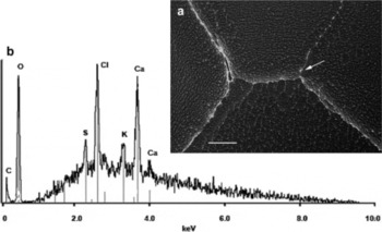
Fig. 8. Vostok 2874 m triple junctions and grain boundaries. (a) SEM image showing an abundance of white spots in grain boundaries (scale bar is 100 μm). (b) EDS spectra from a representative spot (indicated).
In samples from 3399 m, the 5–10μm grain-boundary white spots were of two types. Some, which in one instance coalesced into a line in a grain boundary, had EDS spectra revealing primarily Cl and Na, with small peaks for other elements, including Ca (Fig. 9b). Others contained Ca and S (Fig. 9b). Smaller white spots (1–5 μm) in the lattice contained Si, Al, K and S (Fig. 9b).
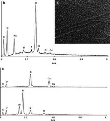
Fig. 9. Vostok 3399 m (a) grain boundary with white spots and thread (scale bar is 100 μm), (b) EDS spectra of small grain-boundary white spots and thread, and (c) EDS spectra of larger white spots on grain boundary (top) and in lattice (bottom).
The 3321.765–3321.805 m specimen was unique because it contained three distinct layers. The top 20 mm and bottom 3 mm are especially fine-grained, while the middle 17 cm (3321.785–3321.802 m) is composed of relatively larger grains, but even these are smaller than would be expected for this depth. Hence this middle layer is referred to as the ‘larger-grained layer’. The top and bottom finegrained layers are termed fine-grained layers 1 and 2, respectively. While all three layers shared the single-maximum fabric and misorientation angle distribution shown in Figure 6 (the orientations of approximately 50 grains in each layer were measured independently), they were different in the type and location of their impurities.
Fine-grained layer 1 (3321.765–3321.785 m) had 5–10 μm grain-boundary white spots containing Si, Al and Mg (Fig. 10a). Some white spots also contained S and Cl (Fig. 10b), while others contained K and Ca (Fig. 10c). This layer also had large 5–10μm white spots in the lattice, containing Si, Al, K and Ca.

Fig. 10. Vostok 3321 m fine-grained layer 1 (3321.765-3321.785 m) (a) white spots on grain boundaries and in the lattice (scale bar is 100 μm), and (b, c) EDS spectra for grain-boundary spots.
Fine-grained layer 2 (3321.802–3321.805 m) had 5– 10 μm white spots on the grain boundaries and in the lattice (Fig. 11a), all of which contained Ca, Cl, K and S (Fig. 11b). This layer also has very large particulates in the lattice, which contained Si, Al, Cl, Ca and C.

Fig. 11. Vostok 3321 m fine-grained layer 2 (3321.802-3321.805 m) (a) white spots on and near grain boundaries (scale bar is 100 μm), and (b) associated EDS spectra (representative of all points indicated).
In the larger-grained layer in the middle (3321.785– 3321.802 m) the white spots on the grain boundaries were smaller (1–5 μm) (Fig. 12a) and contained Cl, K, Si, Na and S (Fig. 12b). No Ca or Al was found in white spots in the lattice or grain boundaries of this larger-grained layer.

Fig. 12. Vostok 3321 m larger-grained layer (3321.795-3321.802 m) (a) grain boundaries and triple junctions, and (b) EDS spectra of white spots on grain boundaries.
Larger impurities, typically 10–50 μm, observed in the SEM, which rarely move during analysis and which have a defined shape, are termed particulates. Many samples of the Vostok core had particulates in the lattice which most often contained Si and Al, often K, Na and Ca, and sometimes Cl, Mg, Fe, S and even Ti. When present, these particulates are generally evenly distributed across the sample surface, and their location is not correlated with grain boundaries. Examples are shown in Figure 13. Details are lost with magnification above × 3000 when examining uncoated ice, so, to examine the particles in more detail, meltwater was filtered through a 0.1 μm cellulose filter and the remaining particles examined in the SEM at 20 kV. A typical insoluble particle obtained this way is shown with its spectra in Figure 14. A thin layer of gold was sputtered onto some samples to eliminate the effects of charging on the image. A specimen prepared this way is shown, with its associated spectra, in Figure 14c and d.

Fig. 13. Examples of particulates in lattice of 3321 m Vostok 5G core specimens. (a) Particulates in the lattice (scale bar 100 μm) and (b) associated EDS spectra. (c) Particle-containing rods (scale bar 10 μm) and (d) associated EDS spectra for body of particle (top) and rods (bottom).

Fig. 14. Vostok 5G 2874 m. Dust on cellulose filter, obtained from meltwater. (a) Dust particle (55 μm across) and (b) its associated EDS spectra. (c) Dust coated with a thin layer of gold prior to examination in the SEM (scale bar is 10 μm) and (d) associated EDS spectra.
4. Interpretation and Discussion
4.1. Texture
The crystal or grain size (area) in many polar ice cores initially increases linearly with the age of the ice (Reference Gow and WilliamsonGow and Williamson, 1976; Reference Duval and LoriusDuval and Lorius, 1980) according to the grain-growth equation (Reference BeckBeck, 1954):
where ![]() is the mean grain area at time t and
is the mean grain area at time t and ![]() is the average initial grain cross-sectional area at pore close-off. The growth rate, K, is temperature-dependent and obeys an Arrhenius-type relationship as shown in Equation (3) (Reference GowGow, 1969; Reference Duval and LoriusDuval and Lorius, 1980; Reference Alley and WoodsAlley and Woods, 1996):
is the average initial grain cross-sectional area at pore close-off. The growth rate, K, is temperature-dependent and obeys an Arrhenius-type relationship as shown in Equation (3) (Reference GowGow, 1969; Reference Duval and LoriusDuval and Lorius, 1980; Reference Alley and WoodsAlley and Woods, 1996):
where Q is the activation energy of the growth process, which Paterson (1994) has estimated at 42.4kJ mol–1 based on crystal growth in firn, K0 is a constant, and R is the gas constant. K is related not only to the in situ temperature, T, but also to the intrinsic properties of polycrystalline ice (grain size, shape and orientation distribution) and to the presence of dissolved impurities, particles and bubbles in the ice (Reference AlleyAlley and others, 1986a, Reference Alley, Perepezko and Bentleyb).
The growth rate, K, in Equation (1) can be compared to other published values, such as the values listed in Paterson (1994) for ice crystals in polar firn. For Vostok (–57°C), the author gives 8 × 10⁻⁴ mm2 a–1, from Reference Barkov and LipenkovBarkov and Lipenkov (1984). However, crystal growth rates are strongly temperature-dependent, and the growth rates in Paterson’s table (Paterson, 1994, table 2.5) are for polar firn. Reference GowGow (1969) notes that crystal growth is especially rapid in the top 10 m of the firn due to the effect of a sustained temperature gradient in a slowly accumulating snowpack, and potentially also because, in the firn, crystals grow at the expense of grains. Below 10 m, where temperature becomes more constant, crystal growth is slower. Reference GowGow’s (1969) extrapolation of his data for crystal growth in polar firn showed that rates in Antarctica could be expected to vary by at least two orders of magnitude depending on temperature, from a low of 3 × 10⁻⁴ mm2 a–1 at –60°C to a high of 300 × 10–4 mm2 a–1at –15°C.
In more recent work, Reference Lipenkov, Ryskin and BarkovLipenkov and others (1999) made an attempt to compile and uniformly scale the data from different sources in which grain size had been measured using different methods. Their data came from 18 ice cores from Antarctica and Greenland and included the data that led to their earlier value for growth rate (Reference Barkov and LipenkovBarkov and Lipenkov, 1984). This time, they assumed a single grain size and shape (octahedral) in each sample, in order to derive a simple relationship between grain size and bubble geometry at pore close-off, and scaled the average crosssectional areas uniformly to correspond with this. After such scaling, the grain growth at Vostok was about 3 × 10⁻⁴ mm2 a–1 (personal communication from V. Lipenkov, 2006).
Taken in this context, our grain growth rate of 1.52 x 10⁻⁴mm2a–1 for the limited data we had in the interval 97–3329m is not unreasonable, particularly given the impact of different grain-size measurement techniques. Finally, we note that crystal growth is also affected by stress and that caution must be exercised when comparing actual growth in regions of deformation and non-random fabrics to the normal crystal growth embodied in Equation (2). The growth rate, K, discussed above was calculated using grain- size data from depths associated with varied climatic conditions (temperature and impurity load) and those at which polygonization may be taking place (this matter is addressed later).
The constant A0 in Equation (2) is the mean grain area at pore close-off, while in Equation (1) it is simply the extrapolated mean cross-sectional area at time 0. Because of the transition from snow to firn to ice in the initial 110 m of the core, this latter value is of no consequence.
From Equation (2), we see that the Kt term becomes very important for older (deeper) ice;hence differences in grain size between different strata at these depths are likely the result of variations in K rather than due to differences in A 0. While K depends on both the temperature and the activation energy, the temperature varies only gradually with depth, suggesting that it is the activation energy, Q, which must be varying between the layers that exhibit linear grain growth and adjacent ones that do not. Since grain-boundary mobility and grain growth are associated with a decrease in grainboundary energy, we seek to understand what is driving the difference in grain-boundary energy at depths where mean grain area does not fit the linear grain-growth model and the grain size is quite small and flattening more pronounced (see Table 1) compared with that in adjacent layers.
The remainder of this paper will focus on the differences between the 2874, 3321 and 3399m specimens and the other specimens. Although grain size in the 3416 m specimen also falls below the fit line in Figure 3, there are additional factors to consider at this depth. First, there is a possibility that the impurities at this depth have multiple origins (basal as well as aeolian) and that the ice has been disturbed by interaction with the bedrock. Simões and others (2002) suggest that some of the impurities in depths between 3311 and 3538 m, and particularly below 3450 m where the mode of volume size distribution shifts and particles too large for aeolian origin (~30 μm in diameter) are found, may be attributable to the ice-bed interface.
Second, the temperature at 3416 m is high enough for migration recrystallization to take place. We do not see signs of this in crystal shape, i.e. interpenetrating crystals (Fig. 2), but have to consider that the elevated temperature at this depth may play some other role in the grain growth there (i.e. because the eutectic point for NaCl, as one example, is -21.2°C). We also note that this depth falls between the glacial stages 14 and 16 identified by previous authors (Simões and others, 2002; Reference Salamatin, Tsyganova, Lipenkov and PetitSalamatin and others, 2004), and represents interglacial stage 15.
4.2. Fabric
The fabric at depths of 97 and 248 m is random (Fig. 6). At 399 m, the distribution of poles also appears random, but the smaller grain size (Table 1) at this depth than at 248 m and its dating (20160 years BP; Table 1) from the Last Glacial Maximum (LGM) suggest that this is a glacial layer. A vertical-girdle fabric is apparent at 650 m and increases in strength with depth. This is consistent with Reference Lipenkov, Barkov, Duval and PimientaLipenkov and others (1989) who demonstrated c axes ‘quasi-uniformly distributed’ in the upper 350 m of the core, trending toward clustering around the vertical plane at 454 m and developing into a strong vertical girdle by 2080 m. The pole figures in Figure 6 show the fabric increasing in strength with depth all the way down to 3416 m, with a few notable exceptions (2874, 3321 and 3399 m). These results for the deeper core (i.e. 3311 m) are consistent with that of De La Chappelle and others (1998) for 3316 m, as well as with that of Reference Lipenkov, Barkov, Duval and PimientaLipenkov and others (1989). The fabric and texture exceptions we noted at 2874, 3321 and 3399 m, where a strong singlemaximum fabric accompanies reduced grain growth, are consistent with the layering identified in Reference Lipenkov and BarkovLipenkov and Barkov’s 1998 presentation of the internal structure of the Antarctic ice sheet at Vostok station (Fig. 1). Hence we follow their naming convention and refer to the fine-grained single-maximum layers as B-type.
At the depths identified as zone C (3310–3370 m) we found two A-type layers (3311 and 3329 m) separated by a B-type (3321 m) layer. This layering could be the result of folding, evidence of which was reported by Simões and others (2002) at 3311 m, but the dark bands we observed in the 3321 m specimen are not tilted and there is nothing else to suggest that folding is the cause of the A–B–A layering here. What Lipenkov and Barkov characterize as zone C could simply be A3 (extending to at least 3311m), B3 (extending from A3 to at least 3321 m) and A4 (beginning by 3329 m).
4.3. Comparison with fine-grained layers in other deep cores
The variation in crystal size, specifically the sudden decrease in size at certain depths, can be compared with similar phenomena noted in the Greenland Icecore Project (GRIP) and Dome Fuji (Dome F;Antarctica) deep cores. Reference Thorsteinsson, Kipfstuhl and MillerThorsteinsson and others (1997) analyzed the correlations between crystal size, δ18O and impurities in the GRIP core and demonstrated that grain size was larger in warm interstadial periods, grain growth was slower during the Wisconsin period, and fine-grained ice was found where calcium and chloride concentrations exceeded 12 and 20 ppb, respectively.
In a comprehensive study of crystal texture and fabric in the Dome F core, Reference AzumaAzuma and others (1999) found that crystal size (defined as equivalent area diameter) increases steadily with depth over the 2500m core, with notable exceptions at five discrete depths, and that crystal size is positively correlated within the oxygen isotope levels. Further, the Dome F layers with smaller than expected crystals had calcium and chloride concentrations of <40 and <100 ppb, respectively (Reference Watanabe, Kamiyama, Motoyama, Fujii, Shoji and SatowWatanabe and others, 1999).
Because the GRIP and Dome F cores come from different geographical locations than the Vostok core, it is not as straightforward to compare their crystal orientations. Fabric develops in response to the local state of stress. At a dome, the vertical compression is accompanied by horizontal extension in all directions, producing a single-maximum fabric. Although the GRIP coring location was at the summit of Greenland, it was also on a dome, hence the shallower ice is primarily under vertical compression and characterized by a single maximum. Simple shear (pure shear plus rigid-body rotation) is caused by glaciers moving over local variations in topography and by substratum debris, but occurs well above the substratum in most cases (Alley, 1992; Reference Thorsteinsson, Kipfstuhl and MillerThorsteinsson and others, 1997; personal communication from R.B. Alley, 2006). It also results in a vertical single-maximum fabric (Reference Alley and WoodsAlley, 1992). Thus in both the GRIP and Dome F cores, the c axis orientation (measured with optical methods) develops from random near the surface to a strong single maximum at depth (Reference Thorsteinsson, Kipfstuhl and MillerThorsteinsson and others, 1997; Reference AzumaAzuma and others, 1999). At an ice divide or a location with significant horizontal flow, such as Vostok station, the dominant mode of deformation is pure shear, vertical compression plus uniaxial horizontal tension (Paterson, 1994). Pure shear can be resolved into principal stresses that are inclined to the surface, and results in a girdle-type fabric. In the Vostok core, the predominant girdle-type fabric makes the presence of a single-maximum fabric in the fine-grained layers above 3450 m (the D layer) notable.
4.4. Possible explanations for microstructural variations
There are several mechanisms capable of limiting grain growth in specific regions of a core: migration recrystallization, polygonization and boundary pinning. Reference Alley, Gowand and MeeseAlley and others (1995) discuss in detail how c axis fabrics can be used to determine which of these is most responsible for limiting grain growth in a given core section. Below, we use a similar analysis, expanded to include the use of a axis information, to determine the cause of microstructural variations in the Vostok core.
4.4.1. Recrystallization
Slower than expected growth in mean grain area, and hence small grain size, can be caused by two recrystallization mechanisms, both of which have an effect on the fabric. First, nucleation and growth of strain-free grains at the expense of older, larger-strained grains containing multiple dislocations, sometimes known as migration recrystallization, is often found near the bottom of cores where it is favored by high strain energy and warmer temperatures. Migration recrystallization has produced both ring and multi-maxima c axis fabrics in laboratory ice (Reference Budd and JackaBudd and Jacka, 1989), but, in nature, the fabric resulting from migration recrystallization probably depends on that of the preceding (shallower) ice as well as on the local state of stress. Migration recrystallization is most likely to take place where the ice temperature is ≤–10°C and, once established, to extend to the bottom of the meteoric ice (Reference AlleyAlley, 1988). Temperatures in the Vostok core do not reach –10°C until approximately 3300m (see Fig. 1). At 2874 m, where the first B layer is noted (B1 in Fig. 1), temperatures are close to –20°C. Further, this B layer and that at 3321 m are discrete and followed by A layers. Even at 3416 m, where the temperature is above –10°C, we do not see the interpenetrating grains that are symptomatic of migration recrystallization (Fig. 2). When drilling had reached 2083 m, Reference De La Chapelle, Castelnau, Lipenkov and DuvalDe La Chapelle and others (1998) determined that no migration recrystallization had taken place in the Vostok core. Now with specimens available from the complete core, we have found no evidence of migration recrystallization as deep as 3416 m.
Second, polygonization (or rotation recrystallization) might explain the lack of an increase in grain size despite increasing depth and age because it involves the conversion of large grains into multiple smaller ones (Reference Alley and WoodsAlley and Woods, 1996; Reference GowGow and others, 1997; Reference De La Chapelle, Castelnau, Lipenkov and DuvalDe La Chapelle and others, 1998). In the characteristic A-type layers, polygonization would cause a widening of the vertical girdle over that which would otherwise be expected (Reference De La Chapelle, Castelnau, Lipenkov and DuvalDe La Chapelle and others, 1998). Reference De La Chapelle, Castelnau, Lipenkov and DuvalDe La Chapelle and others (1998) compare the fabric at 2080 m in Vostok ice to that produced using a VPSC model (the latter is much stronger), and conclude that polygonization has taken place in the Vostok core. In the misorientation distribution histograms for Vostok specimens from the A layers (1201, 1500, 2082, 2749, 3300, 3311 and 3329 m) (Fig. 6), there are peaks in the 1–10° range in the correlated data (between adjacent grains) that deviate from the overall fabric at these depths (seen in the uncorrelated data). This finding supports the theory that polygonization may have taken place in these Vostok A layers. This in turn means that the average grain size in these layers might actually be less than normal grain growth would cause. It does not, however, account for the especially fine-grained B layers.
The misorientations are largely <40° in the B-layer specimens and this is reasonable for the strong singlemaximum ice because the misorientations between grains with a strong preferred orientation should be relatively low. These specimens do not, however, exhibit an excess of very low misorientation angles between adjacent grains (compared with uncorrelated data) that would suggest polygonization. Therefore, neither migration recrystallization nor polygonization is likely to be the explanation for our B layers.
4.4.2. Impurities: dust
Dust levels are typically much higher at Vostok during glacial periods than interglacial periods, due to increased aridity and surface winds in the desert source regions, reduced atmospheric moisture and greater aerosol fallout, and to changes in atmospheric circulation (Reference JouzelJouzel and others, 1996; Reference PetitPetit and others, 1999). Consistent with this, Table 2 shows that the dust concentration is relatively high at 399 m (the end of the LGM), 2081 m (the previous ice age), 2875 m (glacial stage 8), 3321 m (glacial stage 12) and 3401 m (glacial stage 14) (Reference PetitPetit and others, 1999; Simões and others, 2002).
It has been shown both theoretically and empirically that inert second-phase particles inhibit grain growth and grainboundary migration in polycrystalline materials, including ice (Reference Dunn, Walter and MargolinDunn and Walter, 1966; Reference Gow and WilliamsonGow and Williamson, 1976). Indeed, grain sizes are often found to be smaller in visually dirty ice than in clean ice of the same age (Reference Gow and WilliamsonGow and Williamson, 1976; Reference Duval and LoriusDuval and Lorius, 1980). Initially, a causal relationship was drawn between the increase in particle concentration and the decrease in grain size across the Holocene–Wisconsin boundary in several ice cores (Reference Koerner and FisherKoerner and Fisher, 1979). Later, however, two separate groups (Reference Duval and LoriusDuval and Lorius, 1980; Reference AlleyAlley and others, 1986b) compared the intrinsic driving force for grain growth with the drag force from particles in ice. Reference AlleyAlley and others (1986b) concluded that at the particle concentrations present, the particles had little effect on grain growth in typical clean glacier ice. Even in visibly dirty glacier ice, the higher particle concentration does not always fully explain decreases in grain growth rate. For example, in the 1412.3 m Byrd (Antarctica) ice ash band, particles 4 μm in radius (modal value) were found in a region where the grain radius averaged 1 mm. Based on these values, Reference Alley, Perepezko and BentleyAlley and others (1986b) calculated that the particles should reduce grain growth rates by 11%. However, this did not fully explain the small grain sizes present. Therefore dissolved impurities were also thought to contribute to the decreased grain growth rate.
That higher particle concentration alone does not explain the changes in microstructure in glacial periods is supported by our observations of the fine-scale grain-size variations in the 3321.765–3321.805 m specimen. First, the dark bands do not fully account for the finer-grained layers present, as the extremely fine-grained layers are thicker than the dark bands. Second, the whole section (even the larger-grained portion and the ice which is relatively clear) exhibits slower than normal grain growth, which deviates significantly from the fit. Third, the entire 3321 m specimen is characterized by a single-maximum fabric. Hence the entire specimen is classified as a B-type layer, and there is no evidence that ash bands play a significant role in the microstructure. The cause of the differences in grain size within this depth range may be the differences in soluble impurity content.
4.4.3. Impurities: soluble
Soluble impurities inhibit grain-boundary migration and limit grain growth by segregating to the grain boundaries, where boundary velocity is then controlled by the rate of diffusion of impurity atoms (Reference Wolff and ParenWolff and Paren, 1984). Boundary mobility is inversely related to solute concentration, but the strength of the relationship varies with the solute (Reference Wolff and ParenWolff and Paren, 1984). Different solutes have different critical concentrations at which they cause boundary mobility to shift from the high to low regime. The grain-boundary migration- limiting effect of solutes is most noted in doped laboratory ice where the soluble ions exist in high concentrations (Reference Iliescu, Baker and LiIliescu and others, 2003). It has been found that increasing sulfuric acid concentration from 70 to 170 ppb decreases the grainboundary mobility (and significantly retards the nucleation of new grains) (Reference Iliescu, Baker and LiIliescu and others, 2003).
Many attempts have been made to correlate grain size with various soluble impurities in actual ice cores, occasionally with conflicting results. Based on a study of crystal size variations in two Antarctic cores (Dome C and Vostok), Reference Petit, Duval and LoriusPetit and others (1987) suggested a temperature memory effect, where crystal growth is driven primarily by a built-in ‘memory’ of the surface temperature at the time of deposition. The ‘memory effect’ theory is controversial, but it is interesting to note that, in support of their theory, the authors cite evidence to discount the effect of sodium, sulfates and nitrates on variations in grain growth. However, Reference Alley, Perepezko and BentleyAlley and others (1986b) argue that the reduction in grain growth rate and concomitant reduction in grain size in Wisconsin ice from Dome C, Antarctica, is due to impurity drag resulting from the high concentrations of soluble impurities including sulfate, chloride and sodium. Similarly, Reference Langway, Shoji and AzumaLangway and others (1988) found that reduced grain growth in Wisconsin ice from the Dye 3 (Greenland) core was correlated with higher than usual sulfate and chloride ion concentrations. Paterson later reviewed the characteristics of glacial-period ice from a number of cores and concluded that both chloride and sulfate impede grain-boundary migration and grain growth (Reference PatersonPaterson, 1991).
The ion concentrations in the shallower depths in Table 2 could be compared with those reported by Legrand and others (Reference Legrand, Lorius, Barkov and Petrov1988, figs 1—3). The higher cation concentrations in the 650 and 1849 m samples are attributable to the 20% instrument drift discussed earlier. In the 399 m sample, we measured cation levels about an order of magnitude higher, and Cl— and NO3 — levels three to five times higher, than reported by Reference Legrand, Lorius, Barkov and PetrovLegrand and others (1988). Our values are not unreasonable, however, since age and texture already suggest that this ice dates from the LGM. Other significant variations between our ion concentrations and those of Reference Legrand, Lorius, Barkov and PetrovLegrand and others (1988) are as follows: K+ levels more than an order of magnitude higher at 650 and 1849m;and NO3 — values more than an order of magnitude higher at 1200, 1500 and, particularly, 2082 m. Yet neither these high ion concentrations, nor those noted at 399 m, correlate with any noticeable variations in the microstructure of these samples. Instead, the {0001} pole figures (Fig. 6) reveal a steady development (within the limitations of our data) from 399 to 2082 m of the vertical-girdle fabric that is consistent with previous findings for this part of the Vostok core (Reference Pimienta, Duval and LipenkovPimienta and others, 1988; Reference Lipenkov, Barkov, Duval and PimientaLipenkov and others, 1989).
Let us now turn to an examination of the deeper (>2700 m) specimens with fine grain size, namely 2874, 3321 and 3399 m. In light of the work of Reference Alley, Perepezko and BentleyAlley and others (1986b) and Reference PatersonPaterson (1991), examination of the Na+, Cl–and SO4 2— concentration data (Table 2) in particular shows no consistent correlation between high levels of these impurities and fine grain size. The (10–50μm) impurities found in the lattice, composed primarily of Si and Al, with some combination of K, Mg, Fe and sometimes Na, Ca, Cl and S, are most likely primarily aluminosilicates (e.g. biotite, or black mica, K(Mg,Fe)3(AlSi3O10)(OH)2). This is consistent with the higher terrestrial dust input and particle sizes during glacial periods (Reference Legrand, Lorius, Barkov and PetrovLegrand, 1988; Reference Petit, Mounier, Jouzel, Korotkevich, Kotlyakov and LoriusPetit and others, 1990). These types of particle are found in many samples, including interglacial samples, where they tend to be smaller and fewer in number, and are not associated in location with grain boundaries or triple junctions. Typical glacial-period ice from Antarctica (i.e. Byrd Station) tends to be marked by increases in aluminium and silicon (from aluminosilicate dust), but the presence of the large particulates does not seem to be directly related to grain size.
However, in the glacial layers, there is also a positive correlation between fine grain size and a single-maximum fabric and high concentrations of cations, particularly Ca+ (as measured with ion chromatography). As noted earlier, the high impurity concentration, small grain size and strong fabric are often found together in glacial ice, but in the Vostok core two additional differences between glacial and interglacial ice are present. First, there is not only a strong fabric in the glacial ice, but also a different fabric (single maximum vs vertical girdle) to be explained. Second, in the grain boundaries of these samples, Ca, Cl and sometimes K were found together in white spots of unprecedented number and size (5–10μm). While the EDS does not produce quantitative results, the Ca peak was generally significantly higher than the Cl peak (Fig. 11b). Ice from the Vostok area is known to have calcium concentrations comparable to those in Greenland, which increases significantly during glacial periods (Reference PatersonPaterson, 1991). Hence it is not surprising to find calcium in these specimens.
However, it is unusual to find concentrations of calcium on the grain boundaries. The Ca found in the grain boundaries could be associated with small insoluble calcium particles (e.g. plagioclases ((Na,Ca)(SiAl)4O) (Reference LajLaj and others, 1997)), or arise from soluble calcium-containing compounds such as calcium carbonate (CaCO3) and calcium sulfate (CaSO4). Soluble and insoluble Ca-containing impurities generally have different sources, and a low correlation in their occurrence (Reference LajLaj and others, 1997). Only soluble Ca would be detected by ion chromatography, and there was a higher Ca+ ion concentration found in glacial-period specimens. This suggests soluble calcium sources, i.e. CaCO3 and CaSO4. Calcium carbonate is usually observed in desert aerosols, which contribute especially to Ice Age ice, when continental margins are more exposed by a drop in sea level and wind transport is more effective. In glacial period, is Ca (and Mg) also found associated with the nitrate and sulfate anions (Reference Legrand, Lorius, Barkov and PetrovLegrand and others, 1988; Reference LajLaj and others, 1997). Not only is CaSO4 fairly common in several solid phases, i.e. gypsum and anhydrite, but it, like CaNO3, may be formed in the atmosphere from the reaction between CaCO3 and acidic gases (SO4 and NOx) (Reference Legrand, Lorius, Barkov and PetrovLegrand and others, 1988). Both CaCO3 and CaSO4 are very soluble and could easily contribute the Ca+ ions found on the grain boundaries. However, the calcium on the grain boundaries could also be associated with very small insoluble particles, particularly when found with Na, Si and Al.
The Cl and K found in grain-boundary white spots are also easily explained. Sea salt is very soluble and is the main source of Cl in ice (Reference Legrand, Lorius, Barkov and PetrovLegrand, 1988). Soluble potassium in ice cores comes largely from sea salt and clays, as other terrestrial sources such as K-feldspars (KAlSi3O8) and mica (KAl2(AlSi3O10)(OH)2) are less soluble. Clay (and mica) content is independent of temperature, but K-feldspars are more abundant during cold stages (Reference LajLaj and others, 1997). Hence, it is not surprising to see K occasionally contributing to the white spots found on the grain boundaries of our glacial ice.
To summarize, as Ca was often present in the grainboundary impurities in the B layers (but never in the A layers), and as it was found in higher ion concentration there, and also because high concentrations of Ca are a documented aspect of glacial ice, it appears that Ca is playing an important part in limiting grain growth in those layers. It is also worth noting that of the two most prevalent constituents, Ca has more than twice the atomic radius of Cl (180pm vs 79 pm) suggesting that interactions of the large Ca atoms with the imperfect lattice at the grain boundaries may be affecting grain-boundary migration and grain growth.
It is interesting to note that Ca in the lattice and grain boundaries was found only in the very fine-grained layers of the 3321 m specimen, and not in the larger-grained layer in its middle (3321.785–3321.802 m). The cation data for the 3321 m specimen, showing a relatively significant Ca+content (409 ppb), were measured in samples cutting across all three layers. Although Ca was found in large particulates in the lattice in each layer of the 3321 m sample, none was found in the grain boundaries of the larger-grained middle layer. Perhaps this explains the variation in grain size within this specimen. It would not explain why even the grains in the middle layer are not as large as expected, but their confinement between the two fine-grained layers might.
4.4.4. Influence of orientation on grain growth
The statistically high predominance of certain orientations in a polycrystal also affects grain growth. Here, some clarification of terminology is necessary, because both metallurgical and glaciological literature is referenced. First, the terms crystal and grain are used interchangeably for polycrystalline ice. Second, the crystallographic orientation of grains in an aggregate, known as texture in other materials, is referred to as fabric in geology and glaciology. In materials science, the limiting effect of a strong preferred orientation on grain-boundary migration is known as ‘texture-pinning’. This same terminology is used herein, to mean that a strong fabric (preferred orientation) pins or limits the texture (grain size). Boundary structure, i.e. the lattice site coincidence between the adjacent grains and the orientation of the boundary with respect to the lattices, influences boundary mobility. Two grains with similar orientations share a low-angle grain boundary, which has less energy and mobility than a high-angle boundary (Reference Humphreys and HatherlyHumphreys and Hatherly, 1995). Grain-boundary migration, which involves diffusion processes across the boundary, is required for grain growth. When a high percentage of the grain boundaries in a polycrystal are of the less mobile, low-angle type, grain-boundary migration, and hence grain growth, is slower than it would be if the specimen were isotropic. Texture pinning has been observed in several metals. For example, measurements on bicrystals of zinc have shown that: the mobility of low-angle grain boundaries (< 10°) is significantly lower than that of high-angle boundaries; mobility increases with misorientation;and the activation energy for low-angle boundary migration is higher than that for high-angle boundaries (Reference Humphreys and HatherlyHumphreys and Hatherly, 1995).
A similar phenomenon may take place in ice. Initially, after pore close-off, meteoric ice is fine-grained and isotropic. Compression from the overburden tends to produce a single-maximum fabric in the ice sheet, due to slip on the basal plane, which rotates the c axes toward the compression axis (Reference AlleyAlley, 1988). At Vostok, the added factor of uniaxial tension leads to the development of a vertical- girdle fabric.
Over time, a vertical-girdle fabric evolves due to the combined effects of basal slip under the effects of horizontal flow and uniaxial tension, and orientation preferred grain growth. Grains with higher-angle grain boundaries have a boundary mobility advantage. This means that, depending on their size advantage or lack thereof, they will grow or shrink compared with their low-angle grain-boundary neighbors. Where higher-angle boundaries exist in the polycrystal, larger grains consume smaller ones, and the average grain size increases.
An example of this can be found in the recrystallization of metals. Reference Li and BakerLi and Baker (2005) found that the primary recrystallization of cold-rolled, high purity nickel at 400°C resulted in a weak cube texture with a lesser {124}(21-1) component. After secondary recrystallization, only the {124}(21-1); oriented grains remained. These outgrew grains with other orientations and consumed them during a growth selection process driven by advantages in grain-boundary energy or mobility. Reference Abbruzzese and LuckeAbbruzzese and Lücke (1986) developed a model for such texture-controlled grain growth. They found that the simple model of a critical radius separating grains that grow from those that shrink fails when orientation is introduced as a factor. Instead, different orientations have different critical radii and, in the presence of preferred orientations, the grain growth law expressed in Equation (2) no longer holds.
4.4.5. The relationship between solutes and orientation
Finally, the relationship between solutes and boundary geometry adds a third factor to boundary mobility. Reference Humphreys and HatherlyHumphreys and Hatherly (1995) go so far as to argue that the orientation dependence of grain-boundary mobility arises from an orientation dependence of solute segregation to the boundary rather than from an intrinsic structure dependence of grain-boundary mobility. In some metals there is evidence that the orientation dependence of mobility decreases at both very high and very low solute concentrations. In zinc, for instance, there is a window in impurity content in which an orientation dependence of mobility is observed (Reference Sursaeva, Andreeva, Kopezky and ShvindlermanSursaeva and others, 1976; Reference Gottstein and ShvindlermanGottstein and Shvindlerman, 1992).
The B layers in the Vostok core are probably the result of a complex interplay of solute and texture pinning. They are distinguished by the presence of abnormally high Ca levels in the grain boundaries. This limits the mobility of the grain boundary (which in itself limits grain growth) and means that high-angle boundaries lack the advantage that they would otherwise have over low-angle boundaries. If this is the case, there is no reason for grains with divergent c axes (i.e. on the higher-angle parts of a vertical girdle) to grow at the expense of the small grain-boundary angle grains near the center of the {0001} pole figure. This preserves both the smaller average grain size and the single-maximum fabric, which itself contributes to further limiting grain growth through texture pinning. Hence, one observes both smaller grains and a strong single-maximum fabric in the B layers. Neither migration recrystallization nor polygonization has taken place in the B zones, and the abnormally high degree of flattening in the B layers is the alternative to polygonization in the face of further strain after a strong preferred fabric has developed.
5. Conclusions
In the Vostok 5G core, two distinctly different types of microstructure, referred to as A and B, after Lipenkov and Barkov (1998), distinguish interglacial from glacial ice. Analysis of specimens from 97 to 3416 m in the Vostok 5G core leads to the following conclusions:
-
1. The characteristic fabric of the Vostok core, the vertical girdle, is noted beginning at 1201 m, and strengthens with depth in the (interglacial) A layers. That this correlation between fabric strength and depth is not more pronounced (and that the actual fabric is not nearly as strong as predicted by models (Reference De La Chapelle, Castelnau, Lipenkov and DuvalDe La Chapelle and others, 1998)) suggests that polygonization may be taking place in the A layers, as also shown by the high number of very low-angle grain boundaries (1–10°) in these layers.
-
2. In the A layers, which are associated with interglacial periods, grain area increases linearly with time. Grain boundaries are typically straight, grains are very regular, and flattening is correlated only weakly with depth. As deep as 3416 m, migration recrystallization has not taken place.
-
3. Dust content is higher in ice from glacial stages (personal communication from V. Lipenkov, 2004), and specifically it is higher in the vicinity of B-layer samples 2874, 3321 and 3399 m. As mentioned in section 1, a number of glaciologists have concluded that high dust content, while positively correlated with small grain size, is not its cause, and the large particles observed here were always in the lattice, never in the grain boundaries. Further, the 3321 m specimen had visible dark bands that did not correlate with the regions of fine grain size. It is still possible, however, that particulates play an indirect role by supplying a soluble impurity.
-
4. Unusual and significant occurrences of Ca are found on the grain boundaries in the B layers and are unique to these layers. This may explain why the B layers have an abnormally small grain size, which is far less than that suggested by the grain-growth fit seen in A layers between 97 and 3399 m, and a strong single-maximum fabric. Flattening, also indicative of limited grain growth, is also more pronounced in the B layers. These differences are visible within 4 cm of vertical distance at 3321.765–3321.805 m, where there is a central layer of larger and more equiaxed grains in which no grainboundary Ca was found.
-
5. The B zones can be explained by a reduction in grainboundary energy and hence grain-boundary mobility, where the presence of soluble Ca above some critical concentration decreases both grain-boundary mobility and its misorientation dependence, leading to a singlemaximum texture. The grain-boundary calcium may come from large particulates containing this element in a soluble form, i.e. CaSO4 or CaNO3, which, as continental dust, are found in greater abundance in glacial periods.
-
6. Despite fine-scale variations in grain size, 3321 m is a B (glacial) zone. The cause of the differences in grain size within this depth range may be the differences in the amount of Ca present in the fine- and larger-grained layers. Ca is present in particulates throughout the specimen, but was also found in lattice white spots of the very fine-grained layers.
-
7. Stratum C (3310–3370m) includes both A-type (3311 and 3329 m) and B-type (3321 m) layers and may actually represent A3 (extending to at least 3311 m), B3 (extending from A3 to at least 3321 m) and A4 (beginning by 3329 m).
-
8. The ice at 3416m probably represents interglacial stage 15. It falls between 3405 and 3440m, glacial stages 14 and 16 identified by previous authors (Simões and others, 2002; Reference Salamatin, Tsyganova, Lipenkov and PetitSalamatin and others, 2004), and has the characteristics of an interglacial layer, i.e. large grains and a vertical-girdle fabric.
Acknowledgements
We thank the US National Ice Core Laboratory for making available the specimens for this study, and V. Lipenkov of the Arctic and Antarctic Research Institute, St Petersburg, Russia, for generously sharing his data, expertise and insights. We also acknowledge the significant help of G. Hargreaves of NICL and J. Quigley of Dartmouth. This research was supported by the US National Science Foundation grant OPP-0440523. The views and conclusions contained herein are those of the authors and should not be interpreted as necessarily representing official policies, either expressed or implied, of the National Science Foundation or the US Government.


