1. Introduction
In recent years there has been significant interest in the state of the cryosphere, because of its sensitivity to climate change. Changes in the cryosphere influence sea level and local climate and are good indicators of climate change. Large parts of the cryosphere, however, lie in remote areas. In only a few places have quantities such as mass balance and terminus location been measured with sufficient temporal and spatial resolution. Satellite remote sensing is a valuable tool for overcoming this problem; it can be used to observe large parts of the cryosphere on a regular basis without the need to actually go there. Decadal-scale changes in the extent of glaciers and ice caps have been monitored with Landsat reflectance images (e.g. Reference Hall, Williams and BayrHall and others, 1992; Reference Hastenrath and GreischarHastenrath and Greischar, 1997; Reference Williams, Hall, Sigurðsson and ChienWilliams and others, 1997). It is less straightforward, on the other hand, to detect yearly variations in mass-balance components. Satellite passive-microwave sensors can possibly detect the amount of accumulation (Reference ZwallyZwally, 1977), although only over regions with dry snow and with little accumulation, and the amount of hoar formation also needs to be known (Reference Abdalati and SteffenAbdalati and Steffen, 1998). As a consequence, this method has not yet been used in practice. Microwave data can also reveal the boundary between dry and wet snow, which is why they have also been used to measure the spatial extent (but not the amount) of surface melt (e.g. Reference Steffen, Abdalati and StroeveSteffen and others, 1993; Reference Mote and AndersonMote and Anderson, 1995).
A quantity often found to relate linearly to the mean specific mass balance (B) is the equilibrium-line altitude (ELA) (e.g. Reference ØstremØstrem, 1975; Reference Hagen and LiestølHagen and Liestøl, 1990). According to Reference ØstremØstrem (1975), this relation can be used to determine B from satellite images that are taken close to the end of the melting season, provided that the boundary between snow and firn (i.e. the equilibrium line) can be detected. Note that we define firn as all snow that is at least 1 year old, to distinguish it from snow that fell in the mass-balance year under consideration. This method has been applied by several authors (e.g. Reference PeltoPelto, 1987; Reference KulkarniKulkarni, 1992), although only a few actually validated the satellite-derived mass balance with ground measurements (e.g. Reference Rott and MarklRott and Markl, 1989; Reference Demuth and PietroniroDemuth and Pietroniro, 1999). There are several reasons for this. First of all, continuous mass-balance records that can be coupled to satellite-derived glacier properties exist for only a few glaciers. Furthermore, satellite reflectance images often clearly show the boundary between ice and firn or snow (e.g. Reference WilliamsWilliams, 1987; Reference Reijmer, Knap and OerlemansReijmer and others, 1999), but snowfall near the end of the melting season can suddenly lower the snowline and hence obscure the equilibrium line. When superimposed ice is present, the equilibrium line lies below the snowline. Apart from this, clouds often limit the availability of reflectance images. Clouds do not pose a problem when radar images are used. The transient snowline is detectable on radar images (e.g. Reference Rott and MätzlerRott and Mätzler, 1987; Reference Adam, Pietroniro and BrugmanAdam and others, 1997; Reference Smith, Forster, Isacks and HallSmith and others, 1997; Reference Brown, Kirkbride and VaughanBrown and others, 1999), but in these studies it has not been related to the ELA or to B. Although these studies show that the firn line at the end of the melting season can be detected, this does not automatically mean that B can be inferred. The snowline, corresponding to the equilibrium line, is clearly visible when no firn is exposed (Fig. 1a). In the other case, the equilibrium line lies above the firn line (Fig. 1b) and may not be detectable due to small albedo differences between firn and snow a few weeks or months old. This has been observed by Reference Rott and MarklRott and Markl (1989) and more recently by Reference Hall, Williams, Barton, Sigurðsson, Smith and GarvinHall and others (2000) and Reference König, Winther, Knudsen and GuneriussenKönig and others (2001).

Fig. 1. Glacier-facies classification for the end of the melting season, based on the age of the material. Superimposed ice is not shown, because in Iceland it is only found sporadically. (a) When the mass balance is much more negative than in previous years, firn is exposed and the equilibrium line lies above the firn line (after Reference Brown, Kirkbride and VaughanBrown and others, 1999). (b) In the opposite case, when snow covers all firn, only the equilibrium line and not the firn line is visible.
Reference Demuth and PietroniroDemuth and Pietroniro (1999) used the known relation between the ELA and B for Peyto Glacier, Canada, to determine B from the satellite-derived snowline position. However, they did this for one year which displayed a lower ELA than previous years. Furthermore, they noted that digital elevation model (DEM) and satellite image resolution can limit the detection of changes in ELA. Reference Rott and MarklRott and Markl (1989) used images from a year with positive B and from a year with negative B. They could delineate the snowline in the year with negative B on Hintereisferner, Austria, but not on neighbouring Kesselwandferner. Another study in which satellite observations are quantitatively coupled to mass-balance observations is from Reference Greuell and KnapGreuell and Knap (2000). For a period of 8 years, these authors find a correlation between the satellite-derived slush-line position and B for the Greenland ice sheet, but the applicability of this relation is limited because of an upper boundary which the slush line cannot exceed.
In this paper, we use mass-balance data and satellite images from several years to analyze the relation between the firn line and the equilibrium line. We also describe a new method to infer B from satellite images, which only requires satellite imagery. This means that it can be applied to any ice cap or glacier. An important aspect of the method is that the whole surface of a drainage basin during the melting season is studied, and not only a specific transition between glacier facies for a specific day. This takes into account all available information about the surface albedo. As a test case we study Vatnajökull, Iceland. For this ice cap there are mass-balance measurements available, with which the satellite images can be compared quantitatively. Vatnajökull is one of the largest temperate ice masses in the world (8200 km2 in 1995) and consists of several domes, large lobes and valley glaciers (Fig. 2). Owing to the position of Iceland in the middle of the North Atlantic storm track, the skies are overcast most of the time, and albedo retrieval is often not possible. This means, however, that if we can use satellite albedo images to retrieve B here, cloudiness will probably not be a problem for ice masses that are less frequently covered by clouds. Because of the size of Vatnajökull, Advanced Very High Resolution Radiometer (AVHRR) images from the U.S. National Oceanic and Atmospheric Administration (NOAA) satellites, which have a resolution of 1.1 km at nadir, can be used. These images are not expensive and have the advantage of being available several times per day, so obtaining good time series is feasible. Both in situ data and satellite data are from the years 1991–99 inclusive.

Fig. 2. Map of Vatnajökull, based on the DEM used for image processing. The DEM has a horizontal resolution of 500 m. Height contours are shown for each 250 m interval. Indicated are the outlets where the mass balance has been regularly measured. The black circles indicate sites where the mass balance has been measured.
2. In Situ Mass-Balance Data
The mass balance of Vatnajökull has been measured with sufficient spatial resolution since 1992 (Reference Björnsson, Pálsson, Guðmundsson and HaraldssonBjörnsson and others, 1997, Reference Björnsson, Pálsson, Guðmundsson and Haraldsson1998a, Reference Björnsson, Pálsson, Guðmundsson and Haraldssonb, Reference Björnsson, Pálsson, Guðmundsson and Haraldssonc, Reference Björnsson, Pálsson, Guðmundsson and Haraldsson1999; Sigurðsson, 1997; personal communication from O. Sigurðsson, 2001). For one drainage basin (Eyjabakkajökull), data from 1991 are available. The data have mainly been obtained over the drainage basins of Eyja-bakka-, Brúar-, Dyngju-, Köldukvíslar- and Tungnaárjökull (Fig. 2). Most measurements were taken at the end of September or the beginning of October. On each outlet, the mass balance has been measured along one or two profiles which capture the altitudinal variation. Figure 3 displays the mass-balance gradient for some drainage basins. It shows that the amount of annual precipitation influences the mean ELA: the ELA varies from about 1050 m (Eyjabakkajökull) to about 1440 m (Köldukvíslarjökull). Eyjabakkajökull lies closest to the coast and receives most precipitation, while Köldukvíslarjökull has a less maritime and drier climate. Because most of Vatnajökull is quite flat, the profiles can be used together with a few additional measurement sites to describe the lateral variation. The mean specific balances of the areas are obtained by interpolation between the measurement sites. For this interpolation, we developed an algorithm that takes into account vertical gradients. A DEM is needed for this feature to work. For each gridpoint of the DEM (displayed in Fig. 2), the algorithm determines the n closest measurement sites within 500 m in altitude from the gridpoint. Then, because of the limited height differences, a linear relation between mass balance and altitude is found for the n measurement sites, with which the mass balance at the gridpoint can be calculated. To smooth discontinuities in the resulting mass-balance field, the contribution of each measurement site is weighted with the inverse of its distance to the gridpoint. The resulting values of B are not very sensitive to the value of n. We therefore use a value of 6, which is the lowest value that gives smooth mass-balance fields. The resulting mean specific mass balances are displayed in Table 1. The data clearly include years with a highly positive B (1992, 1993) and years with a highly negative B (1997, 1998).

Fig. 3. Average mass-balance gradient along the flowlines of four representative drainage basins of Vatnajökull. Each point represents a measurement site. The curve fits are second-order polynomials.
Table 1. Mean specific mass balances (in m w.e.) as obtained by interpolation for different drainage basins of Vatnajökull. The weighted mean for the whole northwestern part of Vatnajökull (“All”) is shown when the mass balance was measured over the largest part of this area. The bottom row displays the means and the standard deviation of each time series

3. Satellite Images: Processing
AVHRR images were purchased from the Satellite Receiving Station at the University of Dundee, Scotland. We selected 107 images taken from April until September that display few clouds over the ice cap (9–15 images per year). Images from the years 1991–94 were taken from the NOAA-11 satellite. Afterwards, the NOAA-14 satellite provided the images. The images cover the melting seasons of most years reasonably well. For 1993, which had a cold summer with high cloudiness, we found the fewest images (9), and only two images that had been taken before 15 July. Most images display clouds, so on a certain image some drainage basins may be largely covered by clouds. Nearly all images were taken close to solar noon so that solar irradiance was large. The solar zenith angle ranged between 40° and 66° on all images, except for one at the very beginning of the melting season. The satellite images need to be processed in order to retrieve the surface albedo. The retrieval method is based on the method of Reference Reijmer, Knap and OerlemansReijmer and others (1999), although there are a few differences. The processing steps are described below and include cloud masking, geolocation, calibration, atmospheric correction, narrow- to broadband conversion, correction for anisotropy of the reflected radiation and correction for surface inclination.
3.1. Cloud Masking
Developing fully automated techniques for cloud masking over snow surfaces is difficult, because clouds can have the same thermal and visible characteristics as snow. There are automated techniques that detect textural characteristics of clouds (Reference EbertEbert, 1987), but these could not be applied to Vatnajökull because they classify some of the glacier’s surface as clouds (e.g. bands of low ice albedo, firn–ice transition). Some authors have masked clouds reasonably well (e.g. Reference GesellGesell, 1989; Reference Raschke, Bauer and LutzRaschke and others, 1992; Reference Baum and TrepteBaum and Trepte, 1999) using the reflective and thermal differences that often, but not always, exist between clouds and snow surfaces. Here we make use of the reflective and thermal differences in AVHRR channel 3 (3.55–3.93 μm) and the thermal differences in channel 4 (10.5–11.5 μm) that are often present. We empirically found that the following normalized differential index masks most clouds over Vatnajökull:
where Ci is the raw count level in AVHRR channel i. Depending on the temperature difference with the surface, clouds are mostly discernible from the surface in one or both of these channels. Therefore, R 34 often detects clouds in different thermal ranges, over snow and ice and over bare land as well. For each individual image, we apply a threshold for R 34 to mask clouds. This method does not detect all clouds, so we had to check the images manually for errors. A convenient way of doing this is to compare subsequent images and look at textural characteristics. On some images, a difference between the detected cloud margin and the corresponding change in albedo is present, which is caused by shadow casting. However, this applies only to few images and to small areas. As an example we show channel 1 (operating in the visible part of the spectrum) count number and R 34 for one image (Fig. 4). In the west, bright clouds, obscuring the firn line and the ice-cap margin, are visible over the otherwise dark land surface (Fig. 4a). These clouds are visible in a plot of R 34, even over snow and ice (Fig. 4b).

Fig. 4. Channel 1 count number (a) and normalized differential cloud index (b) for Vatnajökull on 8 September 1996. In both plots the–0.22 contour of the normalized differential cloud index is shown.
3.2. Geolocation
We apply a geolocation to each image by comparing the images to the DEM. The horizontal resolution of the DEM is smaller than the AVHRR pixel size, namely, 500 m. The DEM is given in rectangular coordinates, while the AVHRR images are given in cylindrical stereographic coordinates. Because of this we have to rotate the images slightly around the centre of the ice cap in order to obtain a good fit. Then we fit the ice-cap margin and several height contours from the DEM to AVHRR channels 1 and 3. Channel 1 shows sharp mountain peaks and steep ridges (because of changes in surface albedo), and channel 3 clearly shows the margin of the ice cap (because melting snow and ice, unless heavily debris-covered, are colder than land). We were able to locate these features on most images with an accuracy of one pixel. The accuracy of the geolocation for a few images with a large satellite viewing angle is estimated to be two pixels.
3.3. Calibration
The AVHRR instruments record radiation intensities, which must be converted into radiances. Reference Rao and ChenRao and Chen (1995, Reference Rao and Chen1999) provide calibration coefficients for channels 1 and 2 of the AVHRR instruments aboard the NOAA-11 and NOAA-14 satellites, respectively. These coefficients take into account instrument drift. The radiances are simply converted into planetary albedos at the top of the atmosphere by taking into consideration the solar elevation and the distance between the Sun and the Earth.
3.4. Atmospheric correction
The effect of the atmosphere on the albedo is generally linear:
where α srf,i is the surface albedo in channel i, α pia,i is the planetary albedo in channel i, and ai and bi are constants for channel i that depend on the surface altitude, the solar zenith angle, the satellite zenith angle and the composition of the atmosphere. For a given image and assuming a horizontally homogeneous atmosphere over the ice cap, the constants are only a function of surface altitude (Reference ReijmerReijmer, 1997). This means that we only have to calculate this dependence once for each entire image. The atmospheric correction can then simply be applied to all image pixels, because the DEM gives us the altitude of the surface in a pixel. The constants are calculated by means of a radiative transfer model (Reference Koelemeijer, Oerlemans and TjemkesKoelemeijer and others, 1993) which is based on the model of Reference Slingo and SchreckerSlingo and Schrecker (1982). It takes into account Rayleigh scattering and attenuation by ozone and water vapour, but neglects the effect of aerosols. The model is physically less complex than models such as the 6S radiative transfer model (Reference Tanre, Holben and KaufmanTanre and others, 1992; Reference Fily, Bourdelles, Dedieu and SergentFily and others, 1997; Reference Stroeve, Nolin and SteffenStroeve and others, 1997) but also less time-consuming. When we compare the two models for a representative solar zenith angle and with the same atmospheric profile, the resulting surface narrowband albedos appear to differ very little for AVHRR channel 1, but more for channel 2 (Fig. 5). However, the two differences partially counteract, and, moreover, α srf,1 has a much larger weight in the surface broadband albedo than α srf,2 (see below). Because of this, the surface broadband albedos of the two models do not differ more than 0.012 for the entire range of albedo values. This comparison is made for a surface altitude of 250 m, so the differences will probably be even smaller for most of Vatnajökull, where the altitude is higher and the atmospheric correction smaller. Therefore, we conclude that it is not necessary to use the more time-consuming 6S model. Because the results of both models are not very sensitive to the atmospheric profiles (Reference ReijmerReijmer, 1997; Reference Stroeve, Nolin and SteffenStroeve and others, 1997), we use the standard Sub Arctic Summer Profile of Reference McClatchey, Fenn, Selby and GaringMcClatchey and others (1972) as input.

Fig. 5. Difference between the surface albedo from the 6S radiative transfer model and from the Reference Slingo and SchreckerSlingo and Schrecker (1982) model as a function of planetary albedo. For both models, the same solar zenith angle (about 50°), surface elevation (250 m) and atmospheric profile were used. The zenith angles are representative of the images used in this paper. Differences are shown for the AVHRR channels 1 and 2 narrowband albedos.
3.5. Narrow- to broadband conversion
The surface narrowband albedos that are measured in AVHRR channels 1 and 2 have to be converted into a broadband albedo over the solar spectrum. Here we use the empirical expression (personal communication from W Greuell, 2001)
where α srf is the surface broadband albedo. This expression is based on many (8000) point measurements that were made simultaneously in AVHRR channels 1 and 2 and over the entire solar spectrum. Incoming fluxes were measured on the ice-cap surface, and outgoing fluxes were measured from a helicopter that flew at low altitude over Vatnajökull. Methods and data from this experiment are described in Greuell and others (in press). A broad range of surface types was observed, ranging from dirty glacier ice to melting snow and having broadband albedos between 0.05 and 0.80. Equation (3) corresponds very well to the data, with a residual standard deviation of 0.008. Measurements over dry snow are not available, but during the melting season dry snow hardly occurs on Vatnajökull.
3.6. Anisotropic correction
Snow and ice reflect solar radiation anisotropically, so the satellite-derived albedo depends on the view geometry. The function that describes the reflection of solar radiation as a function of the view geometry is called a bidirectional reflectance distribution function (BRDF). It varies with wavelength, solar elevation and (sub) surface properties such as grain-size and impurity content (e.g. Reference WarrenWarren, 1982; Reference Nolin and StroeveNolin and Stroeve, 1997). Liquid water has an indirect effect because it enlarges the effective grain-size. Although existing theoretical models take these effects into account (e.g. Reference Fily, Bourdelles, Dedieu and SergentFily and others, 1997; Reference Nolin and StroeveNolin and Stroeve, 1997; Reference Leroux, Lenoble, Brogniez, Hovenier and de HaanLeroux and others, 1998), it is not (yet) possible to extract independent information about grain-size, water content and impurity content from satellite imagery. We use an empirical BRDF (Reference KoksKoks, 2001) that is based on measurements above melting snow 2 or 3 weeks old and is valid for a broad range of solar zenith angles (15.9–65.5°). The methods and derivation of this BRDF are nearly the same as in Reference Greuell and de Ruyter de WildtGreuell and De Ruyter de Wildt (1999). The measurements were made in Landsat Thematic Mapper (TM) bands 2 and 4, but following Reference Greuell and de Ruyter de WildtGreuell and De Ruyter de Wildt (1999) we can argue that they are also applicable to AVHRR bands 1 and 2, respectively. During the summer, virtually all surface snow of Vatnajökull is melting and metamorphosed, so the parameterization is likely to be valid for the average summer conditions on Vatnajökull. The parameterization is given in the Appendix.
Reference Greuell and de Ruyter de WildtGreuell and De Ruyter de Wildt (1999) present empirical BRDFs that were measured over ice on Morteratschgletscher, Switzerland. It is, however, questionable whether these are applicable to Vatnajökull. Glacier ice may contain air bubbles, dust inclusions and cracks that influence anisotropy. Moreover, much of the glacier ice of northern Vatnajökull (Dyngjujökull and large parts of Brúar- and Köldukvíslarjökull; see Fig. 6) is partly or entirely covered by volcanic deposits, called tephra, which reflect solar radiation more isotropically than snow and ice. For these reasons we did not apply any corrections for anisotropy over glacier ice and tephra-covered glacier ice.

Fig. 6. Six selected NOAA AVHRR albedo images for summer 1996. Each image shows the margin of Vatnajökull (dashed line) and the 0.35 albedo contour (solid line). In the last image (20 September) the equilibrium line is also plotted (inner dashed line). The equilibrium line is obtained by interpolating the mass-balance measurements, as described in the text. Because the mass balance was only measured over the northwestern half of Vatnajökull, no equilibrium line is plotted in the south and southeast.
3.7. Correction for surface inclination
In the above, the fluxes are calculated with respect to a horizontal plane. This means that over a horizontal surface the calculated albedo is the actual surface albedo. However, if the surface is inclined, the fluxes through a plane parallel to the surface differ from those through the horizontal plane, and a correction needs to be applied to obtain the surface albedo. We calculate the surface albedo with the expression of Reference Knap, Brock, Oerlemans and WillisKnap and others (1999). This expression is only valid for isotropic reflection, so we only apply it over glacier ice. Over snow surfaces, the surface inclination is taken into account by applying the correction for anisotropy with respect to the inclined surface.
4. Satellite Images: Results
4.1. Development of the surface albedo during the summer
Figure 6 displays some images with few clouds of the summer of 1996. The images show a gradual decrease of the albedo in the accumulation area, from about 0.8 to about 0.6, and a gradual rise of the snowline. In August this rise comes to a standstill, and the situation remains stationary until the end of the melting season. This is probably a consequence of the albedo of firn being close to the albedo of relatively old snow. The albedo is more constant in time in the ablation area than in the accumulation area. In the northern and northwestern ablation areas, the albedo is very low (around 0.1) and quite homogeneous, due to the tephra covering the ice in this region. Zones with clean ice do occur (Reference Larsen, Gudmundsson and BjörnssonLarsen and others, 1998), but they are not resolved by the AVHRR images. In the south and southeast, the albedo of the ablation area varies considerably on the satellite pixel scale and lies between 0.15 and 0.35 (Fig. 6). On a smaller scale there is even more variability in these regions (Reference ReijmerReijmer, 1997).
4.2. Errors
All processing steps introduce some uncertainty in the surface albedo. The uncertainties resulting from most processing steps are not very large: less than 0.05 (Reference ReijmerReijmer, 1997). The uncertainty introduced by neglect of anisotropy over ice and by the correction for anisotropy over snow is hard to quantify. It will be largest for large satellite zenith angles and extreme surface types (either extremely wet and metamorphosed snow or dry snow). From the information available about BRDFs (e.g. Reference SuttlesSuttles and others, 1988; Reference Stroeve, Nolin and SteffenStroeve and others, 1997; Reference Greuell and de Ruyter de WildtGreuell and De Ruyter de Wildt, 1999) we estimate the uncertainty to be 0.15 in extreme cases but considerably smaller for most images and locations.
5. Mass-Balance Retrieval from Satellite Images
5.1. Detection of firn line and equilibrium line
According to Reference ØstremØstrem (1975), it may be possible to infer B from satellite images if the equilibrium line can be detected. This idea is based on the linear relation between the ELA and B. We investigate this for two representative outlets of Vatnajökull, namely, Brúarjökull in the northeast and Tungnaárjökull in the west. Figures 7 and 8 display albedo profiles of these two outlets at the end of several melting seasons. Note that there are no profiles for 1999, due to a lack of cloud-free images at the end of the summer. Over Brúarjökull the transition from ice to firn and snow is quite sharp in most years, but over Tungnaárjökull it is often too gradual to be determined accurately. The annual mass-balance measurements on Tungnaárjökull display strong fluctuations superimposed upon a linear increase with altitude, probably caused by snowdrift. Synthetic aperture radar images from the European Space Agency ERS satellites with a horizontal resolution of 33 m (not shown here) show that there is no real firn line on Tungnaárjökull, but rather a transition that occurs in patches. This can partially be seen in the profile over Tungnaárjökull for 1993 (Fig. 8), but mostly the resolution of the AVHRR images is too low to resolve the patches. Both on Brúarjökull and on Tungnaárjökull the transition coincides with the equilibrium line in 1993 and 1994, which were years with a positive B (Table 1). In 1995–98, which were all years with a negative B, the equilibrium line lay significantly higher than the upper ice margin, which means that firn had emerged at the surface. It is also interesting to see that on both outlets the firn line was located at approximately the same altitude in these 4 years (Figs 7 and 8). In consecutive years of negative B the firn line will rise, of course, but only very slowly. The firn line therefore marks a transition between nearly static glacier facies (the wet-snow zone and the ablation area), which is the result of meteorological processes during the last years or decades. Hence, the firn line reflects the mean equilibrium line over several years. The same has been observed by Reference Hall, Williams and SigurðssonHall and others (1995) and Reference König, Winther, Knudsen and GuneriussenKönig and others (2001), who found that the firn line coincides with a radar backscatter boundary related to subsurface glacier facies. On Brúarjökull a second transition was present in 1997 and 1998, the years with the highest equilibrium line (Fig. 7). This second transition coincides with the equilibrium line and we assume that it is the boundary between the snow and firn. However, this higher transition did not occur in all years and not on Tungnaárjökull, so it cannot be used to determine the equilibrium line. Summarizing, the equilibrium line is detectable on satellite albedo images when it is not located above its position of the previous year(s), i.e. the firn line. In years when the snowline retreats far enough to reveal firn, albedo monitoring is of limited use for determining the equilibrium line because of the small albedo difference between snow and firn.

Fig. 7. Satellite-derived albedo profiles along a flowline of western Brúarjökull at the end of the melting season, for several years. The mass-balance measurements from which the ELAs are determined were made along the same flowlines. In 1992, no measurements were made on Brúarjökull, and no suitable image is available for the end of the 1999 melting season. The ELA in 1995 was the same as in 1996. For all years, the image that displays the highest firn line is used to obtain the profiles. Dates: mm-dd-yy.

Fig. 8. Satellite-derived albedo profiles along a flowline of Tungnaárjökull at the end of the melting season, for several years. The mass-balance measurements from which the ELAs are determined were made along the same flowlines. In 1995 and 1996, no measurements were made on Tungnaárjökull, and no suitable image is available for the end of the 1999 melting season. For all years, the image that displays the highest firn line is used to obtain the profiles. Dates: mm-dd-yy.
5.2. Mass-balance retrieval from the integrated surface albedo
The appearance of firn and/or slush with low albedos in warm years obscures the equilibrium line, but at the same time provides extra information that may be used to infer B. For example, the mean albedo of the entire accumulation area depends on the age of the snow and hence on the mass balance in the accumulation area. The mean surface albedo of the ice cap not only reflects the amount of accumulation and ablation in the preceding part of the mass-balance year but also strongly affects net shortwave radiation and hence summer melt. To take this feedback into account, we convert the satellite-derived surface albedo into the net potential global radiation:
where α srf is the satellite-derived surface albedo, Q pot is the potential global radiation, defined as the incoming solar radiation at the top of the atmosphere, and Q pot,net is the net potential global radiation. Q pot,net is the potential absorption of solar energy per unit surface area. This differs from the actual absorption of solar energy (Q net) which is lower due to atmospheric attenuation. However, the satellite images mostly display low cloudiness or no cloudiness at all and are in this respect not representative. Cloudiness strongly determines the amount of solar energy that reaches the surface, but the average cloudiness over a time interval is not known over remote and/or large ice caps and glaciers. Hence it is not possible to retrieve Q net over long time intervals from satellite images, which is why we compute Q pot,net instead. Note that it is necessary to take into account atmospheric effects upon the albedo, because several processing steps in the albedo retrieval process need to be applied upon the surface albedo, and not upon the planetary albedo (e.g. anisotropic correction, narrow- to broadband conversion).
Q pot is easily calculated from standard astronomical theory (e.g. Reference WalravenWalraven, 1978). We propose that Q pot,net, integrated over the ice cap and over the summer, is related to B:
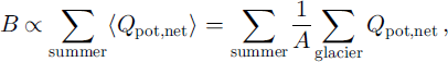
where 〈Q pot,net〉 is the net potential global radiation, averaged over the surface with area A. Equation (5) can be evaluated by simple linear interpolation between the days for which images are available, but this may result in unrealistic curves when few images are available. Also, all images from which 〈Q pot,net〉 is derived may show partial cloud cover, and the visible part of a drainage basin may not be representative of the entire drainage basin. Therefore, we use an analytical expression for 〈Q pot,net〉 that incorporates a priori knowledge about the course of 〈Q pot,net〉 during the summer. We find that the following function fits well to the data (disregarding disturbances by clouds):

where day is the day of the year, and a, b and c are constants. This function resembles a normal distribution and has a maximum magnitude a at day b and approaches zero on either side of this maximum. The constant c indicates the width of the curve. We fit this expression to the satellite-derived values of 〈Q pot,net〉, which are weighted with the percentage of glacier area that is visible. This means that images with few clouds have large weights, and images with many clouds have small weights. As an example we show fits of Equation (6) to the satellite-derived values of 〈Q pot,net〉 for the entire northwest of Vatnajökull (Fig. 9). Deviations from the curve fits are mainly caused by clouds (these data points have small weights) and snowfalls. For example, the high value of 〈Q pot,net〉 on day 224 in 1994 is caused by clouds (84% of the satellite pixels are classified as clouds). The low value of 〈Q pot,net〉 on day 238 in 1996 is caused by high albedos due to recent snowfall. On the image taken at this day, the snowline lies well below the firn line during the weeks before and after this day.

Fig. 9. Satellite-derived net potential global radiation (〈Q pot,net〉) averaged over the northwestern part of Vatnajökull, as a function of the day of the year. Data for several years are shown. The curves are fits of Equation (6) to the data points.
When we use a time-step of 1 day and integrate Equation (6) over the longest period covered by the satellite images in all years (days 146-242), we find that the integrated values of 〈Q pot,net〉 correlate linearly with B (Fig. 10). Prescribing fewer degrees of freedom by setting b and/or c to some value or by using second- and third-order polynomials instead of Equation (6) hardly affects this. When we consider only the albedo instead of Q pot,net the results do not improve either and even become slightly worse, probably because the total amount of solar energy delivered to the surface is disregarded. For all drainage basins the correlation between 〈Q pot,net〉 and B is high (Table 2).

Fig. 10. 〈Q pot,net〉 integrated over part of the melting season (days 146–242), as a function of the specific balance. The average 〈Q pot,net〉 per day during the integration period is shown. “All” indicates the entire area where mass-balance measurements were taken (i.e. all mentioned drainage basins).
Table 2. Statistics for the linear B − 〈Q pot,net〉 regression model. The mean annual precipitation for each drainage basin is also shown. “All” indicates the entire area where mass-balance measurements were taken (i.e. all mentioned drainage basins)

6. Discussion
The methods that lead to the data in Figure 10 all introduce some uncertainty, which must be taken into account to assess the applicability of the B − 〈Q pot,net〉 regression model. The uncertainty in the directly measured B is difficult to assess, and for all drainage basins we will use the same first-order estimate. From comparing different estimates of B we estimate the uncertainty to be 0.25 mw.e., which is a conservative value. The uncertainty due to the regression model ranges from 0.24 m w.e. (the entire northwest of Vatnajökull) to 0.51 m w.e. (Tungnaárjökull). The largest uncertainty is introduced by 〈Q pot,net〉 (Table 2). The source of this uncertainty is two-fold: the satellite-retrieval method introduces an uncertainty, and there is an error associated with the analytical expression for Q pot,net (Fig. 9). The resulting error in the satellite-retrieved specific mass balance (B sat) is computed from the regression coefficient dB/d〈Q pot,net〉. This slope, and hence the resulting error in B sat, tends to increase with precipitation. The total error in B sat ranges from 0.50 m w.e. (Köldukvíslarjökull) to 0.76 mw.e. (eastern Brúarjökull), which is 2–3 times as large as the error in the direct observations of B. It is interesting to note that, just like the error in B sat, the overall range of annual mass balance tends to increase with mean annual precipitation. This range is 1.8–2.8 m w.e. for different parts of Vatnajökull (Fig. 10). The result is that for all drainage basins the ratio between the error in B sat and the range of annual mass balance is nearly the same, namely, 27 ± 3%. Hence, for all drainage basins of Vatnajökull, the satellite retrieval method can only positively detect annual changes in B that are larger than 27 ± 3% of the range of annual mass balance.
The larger uncertainty in B sat also has implications for the possibility of estimating trends and averages. For example, the average B (Table 1) only differs significantly from zero (at the 95% confidence level) for Eyjabakkajökull. For all other drainage basins, more annual measurements than presently available are required to make such a statement. The number of annual measurements needed for this statement (n y) increases when the error in the mass-balance measurement increases, as is the case when the satellite retrieval method is used. The observed variance in B is partly due to natural variability and partly due to the measurement error in B. When we replace the measurement error in B with the error in B sat, we find that for all drainage basins n y becomes about 50% larger.
7. Conclusions
Remote-sensing instruments are useful tools for observing glaciers and ice caps without the need to actually go there. The most obvious feature on the surface of glaciers and ice caps is the transition from ice to firn or snow, which can be successfully observed. However, this boundary is not always equal to the equilibrium line and hence not always related to the mass balance. This is often the case when the equilibrium line is located above its position of the previous year(s), because then firn is exposed, which obscures the equilibrium line. Very small differences in albedo and texture between snow and firn make the equilibrium line hard, if not impossible, to detect in these years. This is especially true when no a priori information is available and one does not know where to expect the equilibrium line. Occasionally, the equilibrium line is visible as a secondary jump in albedo, but this is not the case in all years with a negative B and not on all outlets. Apart from these problems, the ice–snow transition is not always sharp and, depending upon glacier size and climatic setting, satellite and DEM resolution may limit the possibility of inferring changes in ELA from satellite imagery (Reference Demuth and PietroniroDemuth and Pietroniro, 1999). In one year there were too many clouds to find a suitable image of the end of the melting season.
These problems are not encountered when one studies the mean surface albedo of the entire drainage basin during the melting season, and not merely a boundary between two facies on a certain day. In years with a negative B, much relatively dark firn is present, while little summer snowfall and high melt rates may also contribute to a darkening of the surface. In years with a positive B, no firn is exposed, more glacier ice is covered by snow, and summer snowfall may brighten the surface. The albedo feedback (which strengthens the correlation between B and the albedo) is taken into account by weighting the mean surface albedo with the potential global radiation so that the mean net potential global radiation (〈Q pot,net〉) is obtained. By using Q pot,net, and not the global radiation at the surface, one does not need to know the average cloudiness. Consequently, the method can be applied easily to any ice cap and glacier in the world by using satellite data alone. 〈Q pot,net〉 is strongly related to surface melt and also depends on winter precipitation and melt earlier in the melting season. Because 〈Q pot,net〉 varies during the summer, the surface during the whole summer must be studied in order to extract all available information. An additional advantage of studying several images is that one does not need to find one cloud-free image of the end of the summer that is not disturbed by snowfall. We find that 〈Q pot,net〉, integrated over the melting season, is linearly related to B. Due to uncertainties in measurements and methods, this relation can only be used to detect changes in B of at least 0.50–0.76 m w.e. (for different parts of Vatnajökull). This is two to three times larger than the uncertainty in the directly measured B, which implies that more annual measurements are required in order to confidently estimate averages and trends when the satellite retrieval method is used.
The linear relations between B and Q pot,net are based upon data from years with very positive and with very negative values of B. The drainage basins for which these relations are found have different hypsometries, climate settings (different amounts of precipitation) and states of mean balance. Therefore, we expect that yearly variations in B of any ice cap or glacier can be estimated qualitatively with the method presented in this paper. The exact magnitude of yearly variations can only be deduced if the slope of the linear relation is known, and the value of B only if both slope and offset are known. Therefore, the method can be used to estimate B quantitatively for (parts of) Vatnajökull. Note, however, that there is no theoretical ground for the relation between the net potential global radiation and B to be linear for all ice masses. It would be interesting to deduce this relationship for (part of) the Greenland ice sheet (with superimposed-ice and slush zones) and for alpine glaciers (with steeper and more varying slopes). Unfortunately, NOAA images can only be used for ice sheets and ice caps of considerable size. For alpine glaciers images from satellites with a higher resolution (e.g. Landsat) must be used, but these are much less frequently available and are more expensive. This means that the method presented in this work is most suitable for fairly large ice caps and glaciers.
Acknowledgements
We thank W. Greuell for sharing his expertise in image processing and giving useful advice.We also thank A. Brooks and N. Lonie of the Satellite Receiving Station in Dundee for their technical support, selection of images, and patience when we failed to download the images properly. We are also grateful to O. Sigurðsson, two anonymous reviewers and the scientific editor H. Rott for useful comments upon the manuscript. O. Sigurðsson kindly provided mass-balance data for Eyjabakkajökull. C. H. Reijmer purchased some of the AVHRR images. This work was funded by SRON (Foundation for Space Research, the Netherlands), project No. eo-030.
Appendix BRDF Over Melting Snow
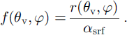
For a given surface type and solar zenith angle (θ s), the bidirectional reflectance (r) that is measured by the satellite sensor only depends upon satellite zenith angle (θ v) and satellite azimuth angle (φ) (relative to the solar azimuth angle). Bidirectional reflectance is related to surface albedo (α srf) through the anisotropic reflectance factor (f):
The parameterization that we use for f over melting snow and firn surfaces reads (Reference KoksKoks, 2001):
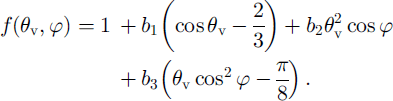
The derivation of Equation (A2) is nearly the same as in Greuell and De Ruyter de Wildt (1999). The factors b 1, b 2 and b 3, which describe the dependence of f upon surface albedo and solar zenith angle, are given by
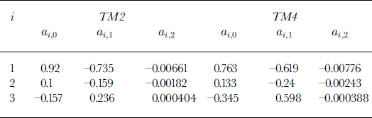
where i is 1, 2 or 3 and θ s must be given in degrees. Values of the coefficients α i,0, α i,1 and α i,2 for Landsat TM bands 2 and 4 are listed in Table 3.
Table 3. Values of the coefficients α i,0, α i,1 and α i,2 in Equation (9). The coefficients are given for Landsat TM bands 2 and 4