


Introduction
One of the prime goals of the Arctic Ice Dynamics Joint Experiment (AIDJEX) is an improved understanding of the drift of the pack ice in the Arctic Ocean. In the past this problem has interested a number of investigators who have attempted to analyze the drift tracks of manned ice stations and beset ships (Reference Campbell and SaferCampbell, 1968). The first of these investigations (Reference Nansen and NansenNansen, 1902) considered a wind stress τ a, a water stress τ w, and a Coriolis force C as the pertinent terms in the momentum equation. More recent work included the gradient current force G and the existence of appropriate boundary layers. All of these forces can be considered to exist at every point on the ice. For small areas of interest, such as the floe on which a given station is located, these forces can, in principle, be measured and expressed in terms of pertinent averages. Even as this work was progressing, field observations clearly indicated a significant lateral transfer of stress through the pack. For example, severe ridging frequently occurred when the local winds were calm. This lateral transfer of stress has been called the internal ice stress I and is the least understood of the forces currently included in the momentum equation ( I is more precisely the divergence of the internal stress field, I =∇· τ). The local value of I is a function of both the regional stress field and the distribution of ice types, as well as roughness elements such as ridges, hummocks, and leads; in short, it is determined by the thermodynamic and strain history of the ice. As new strains occur, the resulting deformation features modify the average roughness of both upper and lower ice surfaces. This changes the values of τ a and τ w exerted on the surrounding pack, which in turn affects I.
The internal ice stress was first treated as a simple frictional resistance by Reference SverdrupSverdrup (1928) and later as an effective viscosity by Reference RuzinRuzin (1959), Reference Reed and CampbellReed and Campbell (1962), and Reference CampbellCampbell (1965). The later approach assumes that on a large scale the ice pack can be considered to act as a thin layer of a Newtonian viscous fluid. Using the viscous model for I, Reference CampbellCampbell (1965) has been able to predict realistic mean drift velocities as well as the actual position for the Pacific Gyre. His results also show how sensitive the mass transport and ice flow fields are to changes in I. Unfortunately his model gives unrealistically high convergence rates for the gyre.
It is possible to conceive of a number of alternative ways to treat the internal ice stress problem (see, for example, the papers in AIDJEX Bulletin, No. 2, 1970). However, without an experimental basis for evaluating the results, it would be difficult to choose among the different approaches. Hence, one of the most urgent needs is for sets of good field observations on the actual deformation of the Arctic ice pack, both under a wide range of ice conditions and on several time and space scales. Because, in principle, it is always possible to measure G, C, τ a, and τ w at the deformation sites, it should, at times be possible to determine I as a residual. The variations in I can then be related to both the regional stress and strain fields and to differences in the large-scale morphological characteristics of the pack in the study areas.
The present paper describes the results of a pilot study of the local deformation of the pack in the vicinity of Camp 200, the site of the 1971 AIDJEX Pilot Project in the Beaufort Sea. The purpose of this study was to test experimental procedures and to obtain information on both the total strain and the variation in the strain-rate that occurred during the occupancy of the stations.
Previous work
To the best of our knowledge, there have been only a few attempts to measure the deformation of the pack ice even though the desirability of making such measurements has been obvious for some time. The reason for this paucity of data is clear: most field parties operating in the Arctic Ocean have been based on only one drifting station and have not had the air support necessary to lay out and monitor strain arrays in areas of active ice deformation.
Two studies of local strains have been made using a theodolite and a base line laid out on an ice island. In 1952 Crary followed the relative motion of several prominent hummocks located in the pack within 5 km of the edge of Fletcher’s Ice Island T-3 (Reference Browne and CraryBrown and Crary, 1958). The relative locations of these hummocks did not change significantly over a five-month period. In addition, between 1962 and 1965 a series of similar measurements was made from ARLIS-II by Reference Senior, Senior, Wittman, Skiles and SaterSenior and others (1968). In the spring of 1962, the relative motion of four towers located within 1130 m of the edge of the ice island was monitored every two to three days for a one-month period. During this time period a lead 9 m wide opened within the array and then closed, forming a 3 m pressure ridge. In the spring of 1963, a larger (nine-tower) array was established and monitored at similar time intervals for 1.5 months. The maximum distance of a tower from one end of the base line was just under 5 km. For the first three weeks, little motion occurred. Then a lead 300 m wide rapidly opened between the base line and the towers. Later, a number of leads 15 m wide developed in the area of the towers. Divergences as large as 0.039 were observed, although most values lay between ±0.01. Similar studies were performed in the spring of 1963 and in the fall of 1963, 1964, and 1965, but no significant relative motion was observed.
The T-3 and ARLIS-II studies share a common difficulty. Ice islands are not typical elements of the Arctic pack. In general, differences in movement between ice islands and the surrounding pack are to be expected. The reason for this is the difference in the roughness of the upper and lower surfaces of the ice island as compared to the ridged sea ice, and the larger Coriolis effect on the ice island because of its larger mass. Sometimes, however, the sea ice near an ice island appears to move as a unit with the island. For example, Senior and others estimate, based on observations from an aircraft, that during much of the period of their strain measurements, the ice within 8 km of ARLIS-II was moving as a unit. In short, unless independent verification is available, strains measured in the vicinity of an ice island are not necessarily representative of strains in the surrounding sea ice.
Reference Dunbar and WittmannDunbar and Wittmann ([1963]) have also measured variations in the areas of the triangle formed by NP-10, NP-11 and ARLIS-II and the quadrilateral formed by these three stations plus T-3. Changes of up to 20% were noted over a 15-day period (the measurement interval), and a maximum change of 63% relative to the initial area was noted over the total period of measurement (four months). The areas involved (roughly 140 000 km2 and 280 000 km2, respectively) were large enough that differences in motion between the ice islands T-3 and ARLIS-II and the surrounding pack would not be significant. Other numerical measures of the deformation were not calculated.
The only study of the relative motion of a station array located completely on pack ice was performed near the North Pole (approximately lat. 88° N., long. 147° E.) during the spring of 1961 (Reference Bushuyev, Bushuyev, Volkov, Gudkovich and LoschilovBushuyev and others, 1967). Four stations were placed in a square with sides of between 75 and 100 km. In general, the stations moved as a block, even down to two small counter-clockwise loops which occurred at roughly the same time (within 6 to 8 h) in each of the otherwise fairly straight tracks. A study of the station velocities clearly indicated that the ice drift commonly preceded the arrival of the actual wind and that the lead time increased with the wind strength. Reference Bushuyev, Bushuyev, Volkov, Gudkovich and LoschilovBushuyev and others (1967) felt that the influence of the wind was transmitted through the ice for at least 150 to 200 km. This again emphasizes the importance of the internal ice stress term in the momentum equation. Although a simple linear relation was shown between the angular rotation of the array of stations and the vorticity of the wind field, no parameters relating to the deformation of the ice were computed.
This survey of previous work reveals that in a mesoscale study of ice deformation one might expect strains of anywhere between zero and several per cent. Because studies have not been made of the homogeneity of pack deformation as a function of the array size, there is little basis for deciding the optimum size of the strain array. Also, little is known about how frequently the deformation array should be surveyed. In the past the most frequent observations were made daily.
Site Location
The site of the 1971 AIDJEX base camp (Camp 200) was on the edge of a large multi-year floe roughtly 16 km across located at lat. 73° 45′ N., long. 130° 15′ W. The general location is shown in Figure 1. The drift of the camp was generally in a south or south-easterly direction with the rate varying from 2 to 15 km/day.

Fig. 1. Position of the 1971 AIDJEX camp is indicated as position 0. Also shown are the locations of the 4 other positions where the surface barometric pressure was obtained so that the wind stress could be calculated. Positions 1, 3 and 4 are located near permanent weather stations. Pressures at positions 1 through 4 were taken from Canadian meteorological maps. The distance a (Equation (13)) was about 320 km.
After an initial aerial examination of the pack in the vicinity of the base camp, it was decided to establish the strain array in the approximately 2 m thick first-year ice to the north-east. The general layout of the strain array relative to Camp 200 and to the major fractures and leads in the vicinity is shown in Figure 2. MRA-3 tellurometers were used as distance-measuring instruments. Distance measurements along the line α–β were obtained beginning on 11 March with complete triangle closures not being made until 12 March. Several closures were made thereafter with the final closure being made on 23 March.

Fig. 2. Overlay of a photo mosaic showing the location of the strain array relative to the major fractures in the area near Camp 200 on 15 March 1971. This photography was obtained by NASA at an altitude of 10 600 m. Multiyear ice, annual ice, and ice islands were identified by variations in surface roughness.
Results
Computational technique
The following procedure was used for determining the strain-rate tensor from the closure data. Consider a medium with the velocity at each point of the medium given by v(x). Since we are concerned only with the horizontal motion of the ice pack, the velocity vector is two-dimensional. Using tensor notation the strain-rate tensor ![]() is defined by
is defined by
To measure the strain-rate tensor we need only to measure relative positions between sets of points, say P and P′, as a function of time. In particular, if we choose a coordinate system such that the line PP′ is oriented at an angle θ to the x-axis, then the one-dimensional strain-rate along pp′, denoted by ![]() , is related to the strain-rate tensor by the equation (Reference NyeNye, 1957)
, is related to the strain-rate tensor by the equation (Reference NyeNye, 1957)
This result is easily obtained by transforming ![]() into a coordinate system with the x-axis parallel to PP′. By measuring linear strain-rates along three or more non-colinear lines, a set of equations of the form of Equation (2) may be solved for
into a coordinate system with the x-axis parallel to PP′. By measuring linear strain-rates along three or more non-colinear lines, a set of equations of the form of Equation (2) may be solved for ![]() . Since in our case only three linear strains were used, the set of equations yielded unique values for the strain-rate tensor so that least-squares averaging was not necessary. (For a discussion of the least-squares solution of Equation (2), see Reference ThorndikeThorndike (1970).)
. Since in our case only three linear strains were used, the set of equations yielded unique values for the strain-rate tensor so that least-squares averaging was not necessary. (For a discussion of the least-squares solution of Equation (2), see Reference ThorndikeThorndike (1970).)
Linear strains
As was discussed earlier, technical problems prevented closing the strain triangle until 12 March. However, on 11 March, an interesting set of detailed readings was obtained between sites α and β. The results are shown in Figure 3. The total strain ϵ is given by
where l
0 is the initial length of the strain line (in this case 8 317 m). Figure 3 shows that after an hour of no variation in ϵ, a rapid extension started with expansions of as much as 0.7 m/min. After 4-5 h, the extension essentially ceased (at 17.30 h) and then quickly started again. If we examine the simultaneous plot of the strain-rate ![]() , we see that it reached a maximum of 0.116 d−l at 15.45 h, then decreased to roughly zero at 17.30 h, then rapidly increased to 0.142 d−l before finally decreasing to a roughly constant value of 0.111 d−1. These events suggest that we saw the transfer of momentum through the pack by jostling between floes.
, we see that it reached a maximum of 0.116 d−l at 15.45 h, then decreased to roughly zero at 17.30 h, then rapidly increased to 0.142 d−l before finally decreasing to a roughly constant value of 0.111 d−1. These events suggest that we saw the transfer of momentum through the pack by jostling between floes.

Fig. 3. Strain and strain-rates on the α–β line, 11–12 March 1971. The small dots along the curve indicate times when the length of the line was measured.
At the time we returned to the Base Camp, the rapid extension was still continuing. When we reoccupied the α–β line at 09.45 h the following day, the value of ϵ was gradually approaching zero, indicating a near return to the state of strain that existed prior to the extension. The maximum period of time over which this extension occurred was roughly 22 h.
Figure 4 shows the strain along the α–β line for the complete period of our measurements. Figures 3 and 4 tell us a great deal about the necessary rate of data acquisition for the mesoscale strain measurements. Daily readings are clearly not adequate: if we had measured the α–β line at noon on 11 and 12 March, we would have concluded that no strains had occurred during this time period. To define clearly an event such as this extension, readings should be taken at least every 8 h. If one wished to examine the fine structure of the event, such as the cusp in the ϵ curve at 17.30 hours on 11 March, readings would be required at least every 15 min.

Fig. 4. Strain on the α–β line, 11–23 March 1971. The solid portions of the curve indicate times when the length of the line was measured.
Strain tensor and strain-rate tensor
The complete strain triangle was measured over a 10 d period beginning with an initial closure at 11.00 h on 12 March. Subsequent closures were made on 15, 21, and 23 March. On all days except 23 March, several sets of closures were made over a period of several hours, allowing strain-rates to be estimated over time intervals of both hours and days. Strain-rates computed over time intervals of a few hours will be referred to as short-term strain-rates, whereas rates computed with time intervals of one or more days will be called long-term. The strain closure data are presented as a function of time in terms of the strains along each leg of the triangle in Table I. Where different strain lines were measured at slightly different times, linear extrapolation was used to estimate strains at the times indicated.
Table I. Net strains along the legs of the strain triangle (units of 10−3)

While the strain measurements were being taken, the direction of true north was determined only approximately (within 5 deg). Consequently, it was not possible to calculate accurate vorticities. Within this error there was no indication of a rotation of the strain array. Therefore, in both long- and short-term strain-rates, the angles between the α–β line and true north were assumed to remain fixed. Even if this is not exactly true, the invariants of the strain-rate tensor will still be correct as they are independent of the coordinate system.
In the strain-rate calculations the vertex angles of the strain triangle were recalculated using the triangle leg lengths at the beginning of each time interval. The net strain tensor was then obtained by summing the differential values of the strain tensor in the north coordinate system.
In one form, the two invariants of a two-dimensional strain-rate tensor are the two components of the tensor along the principal axes (Reference GlenGlen, 1970). The results are presented in this form in Figure 5. The data are presented in the convention often used in glacier flow namely, as two perpendicular lines oriented parallel to the directions of the principal axes. The lengths of the lines are proportional to the magnitudes of the principal axis components. In Figure 5, an outward arrow indicates extension and a bar denotes compression. From the information in this figure, the shear components of the strain-rate tensor in any coordinate system may be constructed. The general trend of the data, with the exception of the strain-rate observed between 12 and 15 March, is an extension in approximately the east–west direction.

Fig. 5. Principal axis component of the strain-rate tensor as a function of time. The long-term rates were calculated using time intervals of two or more days, whereas the other rates were calculated using time intervals of from one to two hours. The directions of the bars indicate the principal-axis directions with their lengths being proportional to the strain-rates.
Another presentation of the two invariants of the strain-rate tensor is the divergence rate ![]() and
and ![]() (in the principal axis system these two invariants are
(in the principal axis system these two invariants are ![]() , respectively). Previous authors (Reference Senior, Senior, Wittman, Skiles and SaterSenior and others, 1968) have reported only the divergence rate, a useful, if not complete, description of the strain. For a direct comparison with previous work as well as for later analysis, the divergence, divergence rate, and shear (y-axis in the north direction) are presented in Figure 6. As can be seen, the long-term divergence rate varies from 0.042 × 10⁻³ h−1 to 0.08 × 10⁻³ h−l. The short-term divergence rate, on the other hand, has values as large as 0.293 × 10⁻³ h−1. This indicates that on the time scale of hours large strains occur which are averaged out when measurements are made over time intervals of several days. The presence of this type of fluctuation is borne out by the detailed measurements along the single strain line α–β as shown in Figure 4.
, respectively). Previous authors (Reference Senior, Senior, Wittman, Skiles and SaterSenior and others, 1968) have reported only the divergence rate, a useful, if not complete, description of the strain. For a direct comparison with previous work as well as for later analysis, the divergence, divergence rate, and shear (y-axis in the north direction) are presented in Figure 6. As can be seen, the long-term divergence rate varies from 0.042 × 10⁻³ h−1 to 0.08 × 10⁻³ h−l. The short-term divergence rate, on the other hand, has values as large as 0.293 × 10⁻³ h−1. This indicates that on the time scale of hours large strains occur which are averaged out when measurements are made over time intervals of several days. The presence of this type of fluctuation is borne out by the detailed measurements along the single strain line α–β as shown in Figure 4.

Fig. 6. The divergence rate, net divergence and net shear as a function of time. The short-term divergence rates were calculated using time intervals of from one to two hours whereas the long-term rates were calculated using time intervals of two or more days.
For a physical interpretation of the divergence, it is useful to recall that when the divergence rate is constant over a region, the divergence rate equals the change in area per unit time divided by the area. From the plot of the divergence in Figure 6, we see that the change in area from 12 to 15 March was about 0.4% with the ice converging, while from 15 to 22 March it was about 1% with the ice diverging.
A useful aid in visualizing the deformation in the strain area during the measurement period is the strain ellipse, which is defined in the principal axis system by
This ellipse has a minor axis in the direction of compression (or least extension) and a major axis in the direction of extension (or least compression). To show the net strain by using this procedure, we have constructed net strain ellipses for 15 March (13.00 h), 21 March (12.00 h), and 23 March (15.00 h)—74, 217, and 268 h, respectively—relative to an assumed circle at time zero on 12 March, 11.00 h. The results are presented in Figure 7 with the principal axis components enhanced by 100. It is clear that most of the strain is occurring along a line approximately in the east-south-east to west-north-west direction.
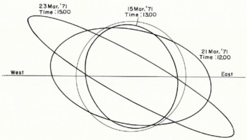
Fig. 7. Net strain ellipses as a function of time. The major ellipse axis is in the direction of maximum extension (or minimum compression) and the minor ellipse axis is in the direction of minimum extension (or maximum compression).
Estimation of errors
The accuracy of the MRA-3 tellurometers when operated at only one cavity tune is better than 0.1 m for differential measurements of distance and for absolute measurements is better than 1 m. In view of this type of accuracy an upper error limit would be 1.5 m over long time intervals (one or more days) and 0.1 m over short time intervals (a few hours). Using these values, the average long-term linear strain measurement error, σ, is 0.02% and the short term error is 0.0013%.
To estimate the variation in the strain tensor components due to such measurement errors, we will assume that the errors are normally distributed with the same variance along each strain line. With these assumptions, the maximum likelihood (Reference Mathews and WalkerMathews and Walker, 1965) values (in the least-squares sense) for the strain-rate tensor are obtained by solving the set of equations of the form of Equation (2). The errors in the strain-rate tensor components within this approximation are given by
where ∆x m denotes the strain-rate tensor errors with
and
Here θ i is the angle between the ith strain line and the east–west axis and L is the transpose of L . For our particular array (using the angles obtained from the first closure) Equation (5) yields
Using the values of σ mentioned above and Equation (5), we arrive at long-term net strain errors for the divergence and shear respectively of 0.047% and 0.029%. For the strain-rate errors, the short-term divergence and shear errors over a 3 h interval are 0.01 × 10⁻³ h−1 and 0.006 × 10⁻³ h−1 respectively. The long-term divergence and shear errors over a 72 h interval are respectively 0.008 × 10⁻³ h−1 and 0.005 × 10⁻³ h−1. These errors are presented as error bars in Figure 6 and, as can be seen, are quite small compared to the magnitude of the strain events. These errors do not, of course, represent the magnitude of the variations in the strain due to lateral inhomogeneity in the strain field (i.e. different strains for different triangles). We expect that such variations would be much larger than the measurements errors. A detailed study of mesoscale strain inhomogeneity is presently under way using data collected in 1972.
Correlation of Synoptic Aerial Photography with the Measured Strains
Aerial photography of the strain triangle and surrounding area was obtained from NASA overflights on 11 and 15 March and by NAVOCEANO overflights on 21 and 23 March. These dates coincided with strain measurements. Unfortunately there was considerable variability in the photography because of changes in the weather conditions, the altitudes flown, and the paths flown. Overlays of mosaics of the area from 15 and 23 March are shown in Figures 2 and 8. Scale and area coverage differences arise from the altitudes at which the two flights were made—10 600 m on 15 March, and 1 500 m on 23 March.

Fig. 8. Overley of an infra-red mosaic of the region near Camp 200 on 23 March taken at an altitude of 1 500 m by NAVOCEANO. The fractures, multiyear ice and thin annual ice were identified by light and bark tones on the infra-red mosaic.
From the photography on which Figure 2 is based, net differences in ice type could be distinguished and are indicated on the overlay. These distinctions were based on the surficial appearance of the different ice types. First-year ice is characterized by sharp angular ridges, with relatively flat ice between the ridges. Multi-year ice shows a freckled appearance caused by its undulating “melt” topography. Ice islands are distinguished by their rolling washboard-like topography and high freeboard. Fractures show as dark lines because of the open water or very thin ice present within them.
Because Figure 8 was made from imagery obtained at a lower level, more detail is present although the area covered is not so extensive. This specific overlay was prepared from an infrared mosaic in which different thicknesses of ice are shown quite clearly because of differences in their surface temperatures. The thickest ice in the mosaic was the multi-year ice (2.5 to 5.0 m). This ice appears dark on the mosaic and is shown in the lower left of the overlay. Lighter tones indicate the thinner first-year ice (up to 2 m thick) that comprised most of the ice in the area of the strain triangle. Within this matrix of first-year ice, two types of thinner ice existed. The thicker of these two made up the refrozen lead 2 000 m wide that crosses the BC–α and α–β lines and is shown by stipple shading in Figure 8. Its exact thickness was not measured, but it is estimated to be ⩾ 1 m. The thinnest ice (0 to 40 cm) occurred in the fracture systems that were active during the strain measurements on 21 and 23 March. This ice appears as bright sharp lines on the infrared mosaic (highest surface temperature) and is shown by the dashed lines in Figure 8.
From Figures 2 and 8 it is apparent that the active leads are not strongly affected by ice thickness variations, since on both overlays leads cut through first- and multi-year ice without deflection. One can also see in Figure 8 that the active lead system does not coincide with pre-existing thin-ice areas, possibly because the orientations are slightly different. The thin-ice area showed considerable activity on 11 March and was presumably still a relatively weak zone on 21 and 23 March.
Details of the fracture structure were analyzed by determining the total fracture length in any given direction. Each fracture was broken into straight line segments, from 100 to 300 m in length, and their orientation and length were measured. The total length in each orientation (10° intervals) for each day of imagery was then tabulated and converted to a percentage of the total length of fracture. The results are shown in Figure 9. In addition, the total length was divided by the area covered by the imagery to give a fracture density analogous to the ridge density used by Reference Mock, Mock, Hartwell and Hibler IIIMock and others (1972) and the drainage density often used in hydrology.

Fig. 9. Histogram identifying the fracture orientations obtained from aerial imagery measured in a clockwise direction from the E–W line. Changes in fracture density agree with convergence or divergence of the pack indicated by the long-term strain-rates. Net fracture vectors on March 15 and 21 agree with the direction expected from the short-term strain-rates (Figure 10).
Because strain data and imagery are variable in time, detail, and coverage, the comparisons between them must be made with some care. We can hypothesize, however, that the net orientation of the fractures (if any) should be correlated with the state of stress of the ice pack as manifested by the short-term strain-rate. To make this comparison, a net fracture vector was calculated from the results in Figure 9 by using Krumbein’s method as described in Reference Mock, Mock, Hartwell and Hibler IIIMock and others (1972). This method uses twice the angle of each fracture orientation to convert the 180° distribution to a non-symmetric 360° distribution.
We calculated
and
Here θ is the estimate of the resultant vector direction, r is the resultant magnitude of this vector in percent, and f is the percentage of the total lead length in each orientation category. For a directionally random population, r is zero. Referring to Reference CurrayCurray (1956), who provides a chart for evaluating significant deviations from zero for r, given the total number of samples, we find that in all cases illustrated in Figure 9 we may reject the hypothesis that our sample is directionally random at the 0.01% level. The directions of the resultant vectors are shown by solid arrows in Figure 9.
On two days—15 and 21 March—both short-term strain data and aerial imagery were available For purposes of correlation it is useful to represent the strain on these days by the strain-rate ellipse, which is completely analogous to the strain ellipse presented in Equation (4) except that strain-rates instead of strains are used. As in the strain ellipse, the strain-rate ellipse has a minor axis in the direction of compression (or least extension) and a major axis in the direction of extension (or least compression). The strain-rate ellipses for 15 and 21 March are illustrated in Figure 10. An angular relationship between the major axis of the strain-rate ellipse and the net lead direction may be hypothesized as follows. Once leads are formed, we assume that the deformation of the pack consists of two motions: shear along the leads and extension (or compression) perpendicular to the leads. Consequently, for a diverging strain the major axis of the ellipse would vary from 90° to 45° relative to the lead orientation, with 90° for pure extension and 45° for pure shear. Conversely, for a converging strain the major axis would vary from 0° to 45° relative to the lead direction, with 0° for a pure compression and 45° for pure shear. Using this model, we note that on 21 March (diverging rate) the fracture orientation was at 9° (from true north) and the major ellipse axis was at 68°, with the difference being between 45° and 90° as expected. Conversely, on 15 March, when we observed a converging strain, the lead orientation was at 70° and the major ellipse axis was at 95°, with the difference lying between 0° and 45° as expected.

Fig. 10. Strain-rate ellipses for short term strain-rates on 15 and 21 March 1971.
Although these agreements are qualitative, they do point to a possible way to estimate the direction (within 45°) of the major strain axis from observations of the fracture structure obtained by aerial imagery. This, of course, assumes that it is possible to determine from the imagery whether the ice pack is converging or diverging.
Another correlation might be expected between the long-term divergence rate and the lead density. In particular, if between two days the lead density increased, we would expect that a diverging strain had occurred. A decrease in lead density would indicate the converse. To test this hypothesis, we have calculated the changes in lead density and compared them with the long-term divergence rate. The results are summarized in Table II. As can be seen, there is general agreement, except for the period 21–23 March.
Table II. Observed changes in lead density and the long-term divergence rate of the ice pack during the same time period

We note, however, that the deformation during this period was dominated by a large shear along a single north–south fracture. This fracture can be seen in Figure 11 (see also Reference HartwellHartwell (1972) who gives a detailed catalogue of motions along leads, including this particular shear). This may be a case in which the strain triangle was not averaging deformation over a large enough area to yield correct results. It is quite easy to construct an example of a triangle with only shear occurring along a single fracture which cuts through the triangle. Such an example would yield a positive divergence where no divergence had occurred. The wind-stress data discussed in the next section also indicates that a convergence would have been expected between 21 and 23 March, so that a measurement anomaly may well have occurred.

Fig. 11. Sequential aerial photography showing shear deformation along the lead that crosses the α–β line approximately 1.5 km from β and runs N.N.W.–S.S.E. (see Fig. 8). Left photograph taken on 11 March, right photograph 23 March 1971.
Aerial imagery is useful for documenting the particular type of shearing motion. The measured net shear is indicated in Figure 6. From the measurements it is not possible to determine the exact type of slippage (it could be east–west or north–south). The en-echelon fractures to the north of site β (Figure 8) suggest that eastern floes are moving south relative to the western floes. This conclusion is verified by a detailed examination of the sequential photography (Reference HartwellHartwell, 1972). Such a net shear agrees with the general motion of the Pacific Gyre in that the measurements were taken on the edge of the gyre with the outer part moving more rapidly than the inner part, causing a north–south slippage of the type observed.
In summary, the experience of the 1971 pilot study has made it clear that sequential aerial imagery is a great help in interpreting strain observations in the pack ice. However, because significant large-scale strain events occur during time periods of the order of hours (e.g., the events of 11 to 12 March), it is quite easy to miss these events on synoptic aerial imagery taken at daily or greater intervals. It is also clear that, at present, imagery cannot provide the details needed for short-term correlations with meteorological factors, nor with the actual measurements of divergence, net strains, and—most important—strain-rates that are required for modeling purposes. At the present time, ground stations must still be relied upon for such critical ice dynamics information.
Correlation of Estimated Wind Stress And Strain
To estimate the wind stress field, the wind velocity field was calculated from barometric pressure readings by using the expression
where u and v are the x and y components of the wind velocity, P is the surface barometric pressure, ρ the air density, f the Coriolis parameter, and K 1 and K 2 are positive constants.
The first terms in Equations (8) and (9) represent the geostrophic wind with a modification expressed by the constant K 1 due to the effect of the frictional drag along the Earth’s surface. The frictional drag also causes the surface wind to have a component moving across the pressure isobars from high to low pressure (Reference PetterssenPetterssen, 1969, p. 158) This component is represented by the second term in Equations (8) and (9). The exact values of K 1 and K 2 may vary depending on the surface roughness. Here we are only concerned with qualitative correlations so the exact magnitudes are not critical. The divergence of the wind velocity field by the above equations is given by
Because of the approximate form of the barometric pressure data available to us, it was impossible to calculate meaningful shear components of the wind stress field; we therefore examined only correlations between the divergence of the ice and the divergence of the wind velocity field.
Assuming the wind stress on the ice is proportional to the wind velocity, a compressional stress will be introduced into the ice which is proportional to ∇· v. This may easily be seen by considering adjacent infinitesimal sections of the ice and determining the force one section exerts on another due to the wind velocity gradient. With a constant velocity, for example, there would be no compressive stress because the external shearing force would be the same everywhere (neglecting variations in surface roughness).
To the extent that other external stresses, such as water stress, may be neglected, we would expect the convergence rate to scale with the compressional wind stress, i.e.
where K is some parameter depending on the compactness and the sign of ![]() . Intuitively this result might be expected to apply to very compact ice which is tightly held and cannot move rapidly, so that Coriolis and water-drag forces may be neglected as a first approximation.
. Intuitively this result might be expected to apply to very compact ice which is tightly held and cannot move rapidly, so that Coriolis and water-drag forces may be neglected as a first approximation.
The other extreme approximation that could be made would be to neglect the internal ice stress completely and consider for example unconstrained wind-driven ice on the open ocean. In this case certain theories yield an ice divergence rate proportional to ∇2 P (with a sign opposite to that in Equation (11), D. A. Rothrock, personal communication). Consequently, for purposes of empirical correlation ∇2 P is clearly a useful parameter to compare with the divergence rate, with the sign of the correlation (if any) giving some indication of the internal ice stress magnitude.
To calculate ∇2 P, we utilized the surface barometric pressure at the five locations indicated in Figure 1. With reference to this figure, pressure P 0 (at Camp 200) was provided by Hans Prelkkinen of the Canadian Polar Continental Shelf Project. These pressures were taken two to three times daily and were therefore extrapolated to 6 h intervals for comparison with other data. The position of pressure P 4 was taken to coincide with the location of Sachs Harbour on Banks Island, where surface pressures were available at 6 h intervals through the Canadian Meteorological Service. Other pressures were taken from surface isobaric charts supplied by the Canadian Meteorological Service, with stations 1 and 3 nearly coinciding, respectively, with the Mould Bay weather station on Prince Patrick Island and the Barter Island station on the Alaskan coast. Data were available at 6 h intervals and a time series of pressure data was constructed beginning at 18.00 h, 7 March. All data were converted to G.M.T. minus 6 h, which was approximately the local time at Camp 200. The distance from P 0 to the other pressure locations was about 320 km. From these five pressure values, the Laplacian of the pressure field was calculated by using a finite difference grid with a the distance between the grid points
Since here we are only concerned with examining the proportionality, we took a/2 = 1.
The results are presented in Figure 12 where we have plotted – ∇2 P versus time, together with the divergence and divergence rate as functions of time. To smooth the pressure data, we removed the high frequencies with wavelengths shorter than 24 h by passing a digital, low pass, unity gain filter over the – ∇2 P curve. The filter had a band pass extending from 0 to (1/96) h−1 and a stop band beginning at (1/24) h−1. The filter was designed according to the procedure discussed by Reference HiblerHibler (1971) and had less than 0.6% side-lobe error. Also note that in Figure 12 an extrapolated divergence curve is given for the time period between 11 and 12 March. This extrapolation is based on observations of the lead structure by using aerial photographs as well as ground observations, and is supported by the strain data taken along the α–β line during the same time period.

Fig. 12. The Laplacian of the surface pressure field, the divergence rate, and net divergence as functions of time. The unit length referred to is about 160 km. The dots on the divergence curve represents actual measurements with the smooth curve simply connecting the measurements. The estimated divergence between 11 and 12 March was based upon visual ground observations, aerial photography, and the linear strain along the α–β line.
As can be seen, a reasonable correlation exists between the wind velocity field divergence and the ice divergence rate. The ice between 10 and 12 March indicated a divergence followed by a convergence which agrees with the estimated wind stress which is positive on the 11 March and negative on the 12 March. The trends of the later data after 15 March are also in agreement with the wind stress divergence generally increasing and the ice divergence rate being positive.
In general, the results presented in Figure 12 are suggestive of a correlation between the negative Laplacian of the pressure field and the ice divergence rate, although the data collected are not sufficient to permit us to make any definitive statements about such a correlation. This is especially true due to the complexity of the ice motion and the neglect of other stresses besides wind stress. Clearly more complete data are needed to investigate whether such correlations are generally noted.
Conclusions
A number of conclusions can be drawn from our study that have considerable bearing on the AIDJEX Project. These are as follows:
-
1. The analysis of mesoscale strains in the ice pack has proved to be of considerable interest. However, for such a study to be of maximum usefulness in the analysis of ice deformation, the strains should be determined at some fixed time interval. The measurements along strain line α–β on 11–12 March suggest that this time interval should be no greater than eight hours. When significant ice deformation is occurring, an interval of 15 min would be even more satisfactory. We do not feel that tellurometers are suitable instruments for such measurements unless they are automated so that only one end of a strain line has to be occupied.
Therefore, during the 1972 AIDJEX field program we will use both continuous-wave and pulsed-laser range finders to determine the distances between the main camp and a series of remote towers.
-
2. It is important that strain measurements be made on several scales so that small-scale floe-floe interactions as well as larger-scale “continuous” deformation of the pack can be analysed and related. Only when such studies are completed can sound statements be made about optimum sizes for strain arrays. An examination of the aerial imagery taken during the overflights (see, for example, Figures 2 and 8) as well as visual surface observations definitely suggest that in most cases the ice divergence as measured within the mesoscale array does indeed correlate with the ice divergence as observed over a larger area. Perhaps such mesoscale strains will serve as an adequate index of the macroscale deformation of the pack.
-
3. The correlations between fracture orientation and the orientation of the strain-rate ellipse, as well as between the lead density and the divergence rate, are encouraging. They suggest that aerial imagery may eventually produce useful quantitative information on the deformation of the ice pack. However, at the present time more combined ground-truth and remote-sensing data will be required both to increase our confidence in such correlations and to make them more quantitative.
-
4. The hope in designing the present experiment was to find simple relationships between the divergence of the wind field and the behavior of the ice. The present results are encouraging. They suggest that detailed mesoscale studies of the relations between the wind flow characteristics and the two dimensional deformation of the ice pack will prove to be most profitable.
Acknowledgements
We would like to thank S. C. Colbeck and S. J. Mock for their helpful comments and J. Riordan and S. Diagneault for their assistance in reducing the data. P. Welsh (U.S. Coast Guard), W. Goddard (University of California at Davis), and D. Williams (Aerojet) helped us man the tellurometer stations. J. Smith and R. Tripp of the University of Washington and K. Hunkins of Columbia University lent us equipment and gave us advice. The men of the Canadian Polar Continental Shelf Project gave us support in a manner to which we would like to become accustomed. The personnel of the NASA and NAVOCEANO aircraft provided us with some fine imagery. Finally, we wish to thank N. Untersteiner, J. Fletcher, R. Bjornert, and the rest of the people at the AIDJEX office for making it possible for us to do this study. This project was funded by the Advanced Research Projects Agency Order 1615.


