


Introduction
The rapid flow of ice streams and outlet glaciers leads to rapid advection of cold ice from the interior of an ice sheet and large deformational heating at the base and sides of the ice stream. These factors, coupled with convergent flow into the ice stream and any subglacial channel, will lead to a complex, three-dimensional ice-temperature regime. This temperature field will affect the deformation of ice through the temperature-dependent flow law and plays a role in the production of basal melting and a temperate layer at the bed. As such, knowledge of the temperature field in an ice stream is important in determining the mechanisms by which the high speeds in the ice stream are obtained.
Knowledge of conditions at the base of a glacier or ice stream, such as the presence of and pressure in water at the bed, the amount of rock debris and its permeability, and the nature of the basal drainage system, is also important for understanding the mechanisms of the flow.For these reasons, several deep boreholes were drilled into the fast-moving Jakobshavns Isbræ, in western Greenland, and instrumented. At a few locations, they reached the bed.
Jakobshavns Isbræ drains approximately 6.5% of the total area of the Greenland ice sheet. Near the calving front, speeds of up to 7 km a−1 are reached. Approximately 25–28 km3 a−1 of ice is calved into the ocean at the terminus (Reference Echelmeyer, Harrison, Clarke and BensonEchelmeyer and others, 1992). Relatively high speeds persist along a well-defined ice stream which extends nearly 80 km inland into the ice sheet (Reference Echelmeyer and HarrisonEchelmeyer and Harrison, 1990; Reference Echelmeyer, Clarke and HarrisonEchelmeyer and others, 1991). A surface velocity of about 1000 m a−1 exists 50 km inland at the location of the drilling. The ice stream lies in a deep bedrock trough, with a center-line depth of up to 2520 m, which places the bed about 1500mb.s.l. (Reference Clarke and EchelmeyerClarke and Echelmeyer, 1989). The large ice thickness, coupled with large surface slopes, leads to high driving stresses and, therefore, high rates of motion.
In the present paper we describe measurements of the ice temperature and water level made in the deep boreholes which were drilled into this glacier. The results are then discussed in terms of the basal hydraulic system and the complex flow regime. A second paper (Part II) describing modeling studies of ice temperature and flow is currently in preparation.
Drilling Operation
In July and August of 1988 and 1989, several boreholes were drilled at three sites designated A, Β and C on a transverse profile across the ice stream, at a distance of about 50 km from the calving front (Figs 1 and 2). The holes were drilled with a hot-water discharge of 60–80 1 min−1. Six to eight oil heating units provided an input-water temperature of 80–90°C. The water was pumped through standard medium-pressure hose (19 mm inner diameter) to a 6 m long drill stem with a nozzle diameter of 4.5–5.5 mm. With this equipment, the time required to drill holes of 0.15–0.20 m initial diameter to a depth of about 1550 m was 20 h. Further details of the drilling method have been described in other papers (Reference IkenIken, 1988; Reference Iken, Echelmeyer, Harrison, Rado and BeaudoingIken and others, 1988). The low ice temperature and correspondingly high freezing rates made it necessary to drill holes with a relatively large initial diameter in order that any instrumentation of a hole immediately after drilling could be successful. For instance, an initial diameter of 0.20 m is required when the ice temperature is −22°C. Reference Humphrey and EchelmeyerHumphrey and Echelmeyer (1990) have investigated the freezing rates of boreholes numerically; that study provided the knowledge of the required hole diameter, and thus the basis for adjusting the drilling speed. At sites A and C, the bed was reached at depths of 1540 and 1630 m, respectively. At the center line (B), the deepest hole was 1560 m, thus terminating 940 m above the bed. The limited capabilities of the drill system precluded drilling 2500 m to the bed along the center line.

Fig. 1. Location of drill sites on Fakobshavns Isbræ. Also shown are velocity vectors and the location of two profiles, I and II, which are referred to in Appendix B. Surface-elevation contours are indicated by light dashed lines. The ice stream is traced with a heavy solid line where distinctly visible, and with a dotted line where the ice stream is difficult to identify. Surface elevation has been modified from that given in an unpublished base map by H. Brecher.

Fig. 2. Location of drill sites on a transverse section through Fakobshavns Isbræ.
A small amount (a few cm3) of bed material was retrieved from the bottom of hole A using small recessions in the drill tip. This material consisted of small angular to rounded grains, ranging in diameter from 0.5 to 3 mm, and some finer material. Examination of the rock fragments indicates a mineral assemblage which includes quartz, biotite, plagioclase and hornblende. These minerals, together with metamorphic structures in the fragments, are characteristic of the biotite-hornblende-gneiss which comprises the bedrock along the coast of Greenland about 50–100 km to the west.
Subglacial Water Pressure
Holes at drill sites A and C (Fig. 2) drained when they reached a depth of approximately 100 m above the bed. The change and stabilization of the water level in each hole was measured with an electrode (well-probe) while drilling continued to the bed. During drilling, water is pumped through the hole; readings of water level taken at this time therefore correspond to a test with a certain constant external water input into the draining borehole. After completion of the hole and shut-off of the external water input, the water-level measurements were continued, showing a renewed drop in water level which eventually stabilized at a new, somewhat greater depth. In the borehole at site C, the water level stabilized at an extrapolated 138.5 m and 141 m depth, with an external input of 80 l min−1 and with no input, respectively (Fig. 3a). The glacier bed was reached at a depth of 1630 m; at this depth a slight reduction of the tension in the drill hose was indicated by a force-meter on the drilling winch. At site A the water levels dropped to much greater depths than at site C: in three different holes (1,2 and 3) water levels stabilized at extrapolated depths of 187, 193 and 199 m, respectively, with no water input. With an input of 65 l min−1 the water levels were 3–5 m higher than these values (as shown, for example, in Figure 3b). The ice depth at site A is 1540 m.

Fig. 3. a. Depth of the water level in the borehole at site C, with a water input from the surface of 80 l min−1 (1.33 × 10⁻³m3s−1) and after termination of this external water input. Time “0” refers to the beginning of drainage in the borehole, b. Depth of water level in borehole 3 at site A, with a water input from the surface of 65 l min−1 and after termination of this external water input. Time “0” refers to the beginning of drainage in this borehole.
At the bottom of a hole which is completely filled with water up to the surface the pressure is higher than in the surrounding ice, due to the different densities of water and ice. At a depth of 1600 m this provides an excess pressure of 1300 k Pa. Such over-pressurization may have caused hydraulic fracturing when a borehole approached the bed; this would explain why the holes drained before they reached the bed itself.
At site C the overburden pressure was 1.46–1.47 × 10⁴k Pa, assuming a mean ice density between 913 and 917 kg m−3. The equivalent depth below the ice surface to the top of a water column is in the range of 142–135 m. Thus, the final water level observed in this hole approximately corresponds to the overburden pressure at the bed. In this case, a small increment of water pressure suffices, locally, to lift the glacier sole upward and to force water into a spreading layer between ice and bed at a high rate.
Various different scenarios for subglacial hydraulic conditions can lead to a water pressure near overburden pressure:
No well-developed subglacial drainage system exists.
A few, relatively large subglacial conduits exist far away from the borehole so that no efficient connection with the borehole can be established.
Or, water flows through deforming subglacial sediments which are relatively impermeable and in which any conduits tend to be filled in by displaced sediment.
Water-level records do not allow us to delineate between these scenarios, and thus, we cannot draw any definite conclusions on the conditions at site C.
At site A the overburden pressure is approximately 1.38 × 10⁴ kPa, corresponding to a water level of 131 m below the surface. The much deeper water levels observed at this site suggest that the holes had connected with a natural, pre-existing subglacial drainage system, functioning at a pressure well below overburden. Moreover, the measurements give a hint about the nature of this drainage system. The relatively small drop in water level observed when the external input to the hole was shut off can be interpreted in two ways:
-
(1) As a pressure drop in a cylindrical channel. In this case, the natural discharge through the channel must have been considerably larger than the additional 65 1min−1 which we added. This is illustrated by a quantitative example in Appendix A.
-
(2) As a pressure drop in a linked cavity network. If bed separation is extensive, water can be stored in growing cavities at a large rate even when the increase in pressure is small. This situation can be expected near the critical pressure. In the idealized case of a perfectly lubricated, sinusoidal bed, the critical pressure, Pc , has been given by Reference IkenIken (1981):

where P 0 is the overburden pressure, T is the basal shear stress and α/λ is the bed roughness. If, for illustration, we take P0 = 1.38 × 10⁴kPa, T = 1.4 × 10² k Pa and α/λ = 0.05, then the critical pressure is 1.335 × 10⁴ k Pa, corresponding to a water level of 176 m below the surface.
Case (2) seems more likely, as it is additionally supported by the observation that the water level stabilized a few meters deeper every time another hole was drilled and began draining through the subglacial drainage system. Flushing with 65 l min−1 for 3 h would not cause a significant perturbation in a conduit which already carries a much larger discharge. However, the natural discharge through a cavity system beneath Jakobshavns Isbræ is likely to be small, especially if it consists of water produced by basal melting only. (Surface meltwater can penetrate the thick layer of cold ice only in very large meltwater streams. The lack of seasonal variations in speed (Reference Echelmeyer and HarrisonEchelmeyer and Harrison, 1990) indicates that little of the surface melt reaches the bed, or, if it does penetrate to the bed by flowing in the necessarily large streams, it affects only a small fraction of the glacier bed.) Thus, the temporary increase in discharge made by our 65 l min−1 input may represent a substantial perturbation in the basal flow regime. This additional input may initiate an unstable growth of the orifices which interconnect the subglacial cavities in a basal hydraulic system similar to that put forward by Reference KambKamb (1987). The growth of these tunnels would tend to reduce water storage and water pressure in such a perturbed cavity system. This would lead to somewhat lower water levels in each successive borehole drilled in the neighborhood of the first hole, as was observed.
A linked cavity system can only exist if sliding of the glacier is substantial. In order to investigate this contribution of sliding to the motion of the glacier, we have analyzed the ice flow near the drill site using finite-element techniques which incorporate the observed temperature profiles. This model suggests that 10–30% of the total surface velocity at this location is due to basal sliding.
Ice Temperatures
The holes were instrumented with calibrated thermistors (accuracy 0.05 K) and tilt sensors, and data were recorded over the winter. The temperature data are shown in Figure 4a and b. At sites A and B, thermistors were lowered to the bottom of the boreholes. In the borehole at site C, however, several thermistors which were attached to the common cable, well above its lower end, were caught at approximately 700 m depth (43% of the total depth). Therefore, the lower thermistors were suspended from this depth, and they reached a maximum depth of only about 900 m. The stated depths of thermistors in this hole (shown by triangles in Figure 4a) may therefore not be accurate.
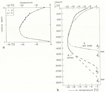
Fig. 4. a. Ice temperature near the margins of the ice stream versus relative depth. Solid dots depict data from site A (southern margin), while the triangles show data from site C (northern margin). Open triangles are drawn where depths are uncertain. Solid line represents a curve through the data at site A only. At site A the total ice depth is 1540 m, at site C 1630 m. b. Ice temperature near southern margin (A) and at the center line (B) versus depth below the ice surface. θ p ′ and θ p are the ice—water equilibrium temperatures with and without air saturation of the water, respectively. The corresponding values of these equilibrium temperatures at the bottom of each borehole are indicated by the horizontal position of the arrows in this figure.
Temperatures measured at the semi-marginal sites A and C are plotted versus relative depth, Z =Z/H (where Ζ is the absolute depth and Η is the local ice thickness), in Figure 4a. These profiles are quite similar. In Figure 4b the temperatures measured near the southern margin, site A, and at the center line, site B, are plotted versus absolute depth. Those latter temperature profiles differ considerably, even though sites A and Β are only 1.5 km apart. At the semi-marginal site, A, the basal temperature gradient is extremely large, 0.1 Km−1, and the temperature minimum of −22.0°C is located at about 1100 m, which corresponds to a relative depth Z (T min)=0.70. At the central site, B, the basal temperature gradient seems to be smaller: extrapolation of the measured part of the profile suggests that the lower part is within the range indicated by the broken lines in Figure 4b. This range includes the possibility of a layer of temperate ice of substantial thickness (up to 400 m), which is shown by the upper broken line in this figure. This upper extrapolation results when the curvature in the lower part of the observed temperature data is considered; the lower broken line does not take this observed curvature into account.
The temperature minimum beneath the ice-stream center line (site B) is −22.1° PC. This minimum is located at a depth of about 1200 m, which corresponds to Z (T min)=0.48. The profile at site Β has a marked bend at a depth of about 200 m; such a bend is less apparent at the semi-marginal sites. This bend may result from a sudden speedup of the ice as it enters the ice stream, combined with a temperature increase at the surface: a distinct velocity increase is expected where the ice stream forms, and this will lead to an increased longitudinal advection of cold ice from higher altitudes. Seismic soundings by Clarke and Echelmeyer (1989; unpublished data, 1990) located the formation of the main ice-stream channel 30 km upstream of the drill site, at an altitude of 1400 m. Less prominent ice streams seem to exist further inland for another 20 km as seen on MOS satellite images, in the surface-feature map of GGU (1987) (personal communication from H. Thomsen), and on an unpublished base map by H. Brecher. Lakes and slush zones are common between 1200 and 1500 m altitude, and cause an increase of near-surface ice temperature (Reference Echelmeyer, Harrison, Clarke and BensonEchelmeyer and others, 1992). The ice which travels in the ice stream passes this warm zone relatively quickly and the effects of this warming reach a shallower depth than in the ice outside the ice stream, which travels more slowly. Thus, the upper part of an ice column is less likely to be in thermal equilibrium with surface warming conditions if it has traveled along the center of the fast-moving ice stream (i.e. site B) than if the column has traveled outside the ice stream (i.e. sites A and C). An anomalous bend near the top of a temperature profile within the ice stream may be formed under such conditions.
Another difference between the temperature profiles at the marginal sites (A and C) and the center line (B) is the difference in the near-surface temperatures, as has been previously noted by Reference Echelmeyer, Harrison, Clarke and BensonEchelmeyer and others (1992). Possible sources for a warmer near-surface temperature at the margins than the center include deformational heating in the shear zones bordering the ice stream and heat liberated upon refreezing of meltwater in crevasses within the shear zones. A third possibility, suggested by T. Hughes (personal communication), and similar to that discussed in the previous paragraph, is the idea that ice within the ice stream comes quickly down from high, cold elevations and has had less time to warm by the time it reaches the elevation of the drill site. The marginal sites move more slowly and, thus, the ice there has had a longer time to warm.
Comparison with a modeled temperature distribution
The temperature profiles shown in Figure 4 are somewhat anomalous in their shape, with large gradients deep in the ice columns, possibly a relatively thick temperate layer in the center of the ice stream, temperature minima at very different relative depths and a sharp bend near the surface. The close similarity between the two semi-marginal sites and differences between these profiles and that at the center are also interesting. In order to understand this structure and its relation to ice-stream dynamics, one must compare the observed temperatures with those predicted by models of varying complexity, each of which should include some facets of the clearly three-dimensional flow and temperature regime.
In the present section, we compare the observed temperature profiles with those obtained from the models of Reference Budd, Jacka, Jenssen, Radok and YoungBudd and others (1982). These authors used several modeling techniques, including moving-column models, with input parameters which included all the surficial glaciological and ice-thickness data available at the time. They produced relatively coarse-resolution (50 km grid spacing) temperature and flow calculations for the entire ice sheet. For direct comparison with our observed profiles, we take the results of Reference Budd, Jacka, Jenssen, Radok and YoungBudd and others (1982) along the approximately 650 km long EGIG—Jakobshavns flowline (their flowline G3, map 4/1 and figures 7.5 and 7.9), from the ice divide down to the coast. In making this comparison, the following assumptions, and some discrepancies in the input data, of the simplified model of Budd and others must be borne in mind:
-
(1) No distinction is made between flow in the ice stream and flow in the ice sheet. No deep bedrock channel beneath the ice stream is accounted for. Furthermore, the specific ice deformation which occurs where the ice enters this channel is not included.
-
(2) Viscous heating due to internal deformation, which should be distributed with depth in the ice column, is replaced by heat sources concentrated at the glacier bed. This is in keeping with their assumption that the horizontal velocity does not vary with depth. Consistent with the latter assumption, the vertical strain rate is also taken to be independent of depth.
-
(3) The input data of the model agree, in general, with what is known at present. However, there are a few important exceptions. (A) Mean horizontal velocities inferred from balance flux (and corresponding surface velocities) appear somewhat low compared to the velocities measured on the EGIG profile, especially along the upper half of the flowline (Reference Budd, Jacka, Jenssen, Radok and YoungBudd and others, 1982, map 4/2). (B) Near the midpoint of the flowline, the surface altitude is about 300 m higher than that given in a recent map derived from satellite altimetry (Reference Bindschadler, Zwally, Major and BrennerBindschadler and others, 1989). (C) Near the coast, the prescribed surface temperatures are too low by several degrees, according to measurements of 12 m temperature by Reference Echelmeyer, Harrison, Clarke and BensonEchelmeyer and others (1992). (D) Mass-balance studies by Reference BenderBender (1984) and Reference Echelmeyer, Harrison, Clarke and BensonEchelmeyer and others (1992) suggest an area of low precipitation which extends at least 100 km inland from the ice margin and encompasses the Jakobshavns Isbræ flowline and much of the drainage basin. In this area, the accumulation is at least 25% lower than along the EGIG line to which Budd’s input refers. The EGIG line approximately follows the northern boundary of the Jakobshavns Isbræ drainage basin.
With these approximations in mind, we have compared Reference Budd, Jacka, Jenssen, Radok and YoungBudd and others’ (1982) modeled ice temperatures with those observed in our boreholes. In Figure 5 the temperatures measured at drill sites A and Β are plotted versus relative depth, together with the model results. Our drill sites are located approximately at 600 km along the flowline from the ice divide in this model. (Near the drill-site location, at 600 km, the estimated ice depth is 947 m according to Budd and others. Outside the ice stream, seismic soundings by Clarke and Echelmeyer (unpublished data) indicate an ice depth of about 1000 m, which is similar to that estimated by Budd and others. As stated above, the bedrock channel itself was not accounted for.) Given this location on the distance scale of the model flowline, the magnitude of the modeled and measured temperature minima are nearly equal. There are, however, considerable differences in the shape of the temperature profile at depth and in the depth of the temperature minima, which, of course, should be expected in light of the remarks (1)–(3), above. The differences are as follows.

Fig. 5. Comparison of observed and calculated ice temperature in Jakobshavns Isbræ and its drainage basin. Heavy lines indicate temperatures measured in the boreholes. The thin lines depict temperatures obtained from the models of Reference Budd, Jacka, Jenssen, Radok and YoungBudd and others (1982, fig. 7.9), with distance from the ice divide indicated.
First, when the ice flows down into the deeply incised channel, a pronounced drop of potential energy occurs, or, equivalently, there is increased ice deformation and heat production. A certain part of the viscous heat production is concentrated in the basal ice. Moreover, while the ice is flowing through the deep channel, heat production near the base, both per unit time and per unit distance downstream, is larger in the ice stream than outside of it. In contrast, the ice in the interior of the ice stream remains relatively cold because it moves along with high velocity and thus is exposed to the warmer environment for only a short time. That is, in the ice stream we expect relatively warm basal ice, with cold ice in the interior. The actual magnitude of the difference between measured and modeled minimum temperature in the interior of the ice is not large. This may be taken as an indication that the ice stream does not extend too far inland from the drill site, although the coarse resolution of the model does not permit us to draw such specific conclusions with any confidence.
Secondly, as a consequence of assumption (2) above, the distance xt from the center of the ice sheet to the point at which the base of the ice reaches the melting point is too small. The model predicts a temperate base well before km 400, that is, more than 200 km upstream from the drill site. Downstream from that point the upward conduction of heat through the basal ice can no longer accommodate the combined geothermal and deformational heat input which, in their model, is supplied at the ice/bed interface. Consequently, much of this heat will go into melting of ice at the bed of the glacier. In reality, however, most of the deformational heat sources are located within the ice. These distributed sources continue to raise the ice temperature until, eventually, a layer of temperate ice may form at the bed which has a non-zero thickness. Because of the large distance between xt the drill site and, because of the increased heat production in the basal ice of the ice stream, it appears likely that a temperate layer of substantial thickness will exist at the drill site. This is compatible with an extrapolation of the central temperature profile (B), which takes the curvature of the observed profile at depth into account. Such a thick temperate layer was not observed at site A.
Thirdly, the discrepancies in the input data mentioned under (3) above, will cause certain deviations of the modeled temperatures from those expected. As a consequence of the low horizontal velocities, the modeled temperatures will be too high near the surface and in the interior, but the difference should not be large. The abnormally high surface altitudes and correspondingly large ice thicknesses will have an approximately equal but opposite effect on the temperatures. The low surface temperatures near the coast will affect the modeled temperatures near the surface only. The higher accumulation rates will cause a slightly higher temperature in the upper half of the ice and a downward shift of the temperature minimum. This shift is, however, too small to account for the difference in depth of the temperature minimum in the model and of that measured at the center line (Fig. 5). Moreover, application of the correct accumulation rates, which are lower, would also increase the discrepancy between the modeled and measured temperature distribution at site A.
The marked differences in the relative depths of the temperature minima remain to be discussed. First, a remark is appropriate as to why the relative depths are compared rather than the absolute depths below the surface. In regular sheet flow, the vertical strain which occurs while the ice flows a given distance along a flowline is, to first order, independent of depth. Thus, where mass balance is negligible, the relative depth of a point within a moving ice column remains unchanged — irrespective of thickness changes of the ice sheet with distance downstream.
In the present problem the flow is more complex; nevertheless, an inspection of relative depths provides a useful means of identifying deviations from a regime of “normal” flow and gradual warming. The differences in relative depth of the temperature minima measured at sites A or C and that measured at site Β have developed in a relatively short time — about 50 years. (This time span refers to the flow of ice in, approximately, the upper 80% of the total ice column.) During that time the ice in the ice stream has traveled a distance of 30–40 km from the ice sheet, through a zone of convergence and along the subglacial trough to the drill site. In the ice sheet upstream of the confluence, the temperature profiles which are characteristics of the flowlines which eventually pass through sites A, Β or C are, of course, equal. The observation within the boreholes (Fig. 4) show that a dramatic change in the temperature distribution takes place as the ice stream develops. Two processes may be responsible for these changes: (1) the large release of heat, which is equivalent to the drop in elevation occurring as the ice flows down into the deeply incised bedrock trough along the ice-stream center line towards borehole Β (the elevation drop is about 1000 m less during flow to the marginal sites A and C), and the upward conduction of this deformational heat, or (2) the complex ice deformation induced by the convergent shape of the sub-surface trough.
In order to estimate the importance of the former process, we put aside the effects of the complex deformation and simplify the problem to a case of “regular” sheet flow. The question then is whether the enhanced dissipation of heat occurring along the center line, where the potential energy drop is the largest, may have warmed the lower half of the ice in such a way that the temperature minimum is shifted upward from a relative depth of 0.70 (as measured at site A, for example) to a relative depth of 0.48, as measured in borehole B. There are two additive mechanisms by which heat can shift the minimum upward, namely warming by the conduction of heat where the temperature profile has a non-zero curvature, and by viscous heat dissipation, which will be concentrated in the less viscous ice lower in the column where the temperature profile is approximately linear. We have estimated the time required for the observed upward shift of the temperature minimum by the conductive heating. The estimated time is in the order of 1000 years, which is much greater than the differential travel time of approximately 50 years. If the assumption that the heat sources are concentrated at the bed holds, then the latter mechanism cannot account for the displacement of the minimum either. Thus, these two mechanisms can be ruled out as the quintessential explanation for the upward shift of the temperature minimum.
We must therefore appeal to the second of the possible explanations for the different relative depths of the temperature minima — namely, kinematic effects in the complex flow regime which exists as deep ice enters the subglacial trough within which the ice stream is located.An important property of this subglacial trough is that it becomes both narrower and deeper in the downstream direction, as illustrated, for example, in Figure 6. The ice at depth, which flows through the trough, will undergo transverse shortening as the valley walls converge. The corresponding transverse strain will be accommodated by both longitudinal extension and stretching in the vertical direction as the deepening trough is filled. The transverse strain is likely to be greater at depth, in the trough, than above it, where the flow is not laterally confined by bedrock walls. Consequently, vertical extension may also be larger at depth than in the ice sheet overlying the trough. The enhanced vertical extension at depth in the channel will then cause the lower part of a temperature profile in the ice stream to be stretched out more than in the upper part. This will displace the temperature minimum upward.

Fig. 6. Diagrammatic sketch of a sub-surface channel which funnels the ice flow.
The actual geometry of the region upstream of our boreholes in Jakobshavns Isbræ is described in Appendix B, along with an estimate of the associated strain field. In that appendix, we show that a significant variation of vertical strain with depth is indeed induced by the special bedrock geometry which occurs in the transition zone from sheet to stream flow. Non-uniform vertical stretching will be more pronounced at the ice-stream center line than at the margins, since the bedrock trough is deepest there. This explains, qualitatively, the differences in relative depth of the temperature minima at drill sites A and B. Because the outlined non-uniform vertical stretching is not included in the models of Reference Budd, Jacka, Jenssen, Radok and YoungBudd and others (1982), one would expect that the modeled temperature minimum is at too great a relative depth in comparison with that measured at site B. This is the case. It does not hold with respect to a comparison with the measurements at site A. A speculative explanation of the latter discrepancy can possibly be given, assuming that the measured temperatures are influenced by remnants of ice-age conditions preserved near the base of the glacier. In contrast, the model assumes a steady state under the present conditions.
We believe that fully three-dimensional modeling is required for obtaining a better understanding of the temperature distribution in the ice stream. Such modeling is also needed for gaining a better understanding of the relative roles of deformational heating and the kinematic distortion of the temperature profiles.
Conclusions
The analysis of borehole measurements described in this paper leads to the following results:
The ice stream is temperate based, at least 50 km inland from its terminus. Moreover, it seems likely that a temperate layer of substantial thickness exists at the base of the ice stream near the center line. The temperate base, combined with the large ice thickness and considerable shear stress at depth (Clarke and Echelmeyer, 1989; Reference Echelmeyer, Clarke and HarrisonEchelmeyer and others, 1991) leads us to expect that the contribution of internal deformation to the motion of the ice stream is large. A quantitative estimate of this contribution will be obtained by flow modeling which takes the observed and inferred temperature distribution within the channel into account (Part II; in preparation by K. Echelmeyer, M. Funk and A. Iken).
A well-developed subglacial drainage system exists near the southern margin. Its relatively low water pressure (or the high effective pressure) is atypical of drainage through deforming sediments. The large storage capacity of the drainage system here makes it possible to accommodate additional water input, as fed into a borehole, without significant pressure increase. This suggests that sliding with extensive bed separation may be taking place in this area.
The temperature minimum is approximately −22.1°C at both the semi-marginal and central drill sites. The relative depth of this minimum, however, is much larger near the margins than at the center of the ice stream. We believe that this results from deformation taking place as ice flowing along the center line enters the deep subglacial channel. In particular, a disproportionately large vertical stretching of the lower part of the ice seems to have occurred by the time the ice reaches the drill-site location along the center line of the channel.
Vertical stretching of the basal ice would have an important consequence: the surface velocity is approximately proportional to the thickness of a basal layer which consists of temperate or nearly temperate ice and which is therefore an order of magnitude less viscous than the ice above it (furthermore, in the case of Jakobshavns Isbræ, the basal ice may contain a layer of “soft” Wisconsin ice, which leads to further softening). Thus, the conjectured vertical stretching of the basal ice could be an important mechanism for the fast flow of Jakobshavns Isbræ and possibly of other ice streams which are funneled by sub-surface channels. Convergent flow occurs below headwalls of various Antarctic ice streams, and there is a speed-up in these convergent zones (Reference McIntyreMcIntyre, 1985).
It is important to investigate this hypothesized kinematic “funnel” mechanism further. Two approaches may be envisioned: one way is to model the temperatures within the ice stream and beside it in detail, with fewer simplifications. Resulting differences between depths of modeled and measured minimum temperatures may then provide a better estimate of ice deformation at depth. Another way is to model the convergent flow directly. Such a model should also indicate the locations where internal heat sources are concentrated when the ice enters the sub-surface channel. Studies along both lines are currently in progress.
Acknowledgements
We wish to thank all who contributed to the preparation and completion of this project. Working conditions in the field were often adverse, for instance, when all pumps froze and the electronic control of the winch failed in a blizzard, requiring the heavy drilling hose to be pulled up by hand or when a drilling-“shift” needed to be extended to over 48 h when there was a malfunction of pumps. The following persons participated in the field work: T. Clarke, D. Cosgrove, P. Gnos, G. Holton, Β. and Η. Jenny, C. Petersen, J. Steiner, T. Thorsteinsson, S. Wagner, R. Wanner and P. Will. Logistic support by the Polar Ice Coring Office, namely K. Swanson and S. Peterzen and their crew, was invaluable. We also acknowledge the support by GTO, Mr H. Bay, in Jakobshavn, and that of several helicopter pilots and personnel of Greenland Air. The manuscript was typed by J. Phillips, C. Gering and by S. á Marca. The drawings were prepared by B. Nedela.
We are grateful to B. Kamb, T. Hughes and an anonymous reviewer for their thorough comments, which helped improve an earlier version of this manuscript.
This project was supported by the U.S. National Science Foundation (grant No. DPP 87–22003) and the Schweizerischer Nationalfonds (No. 2000–5.431).
The accuracy of references in the text and in this list is the responsibility of the authors, to whom queries should be addressed.
Appendix A
In the following, we will estimate the discharge in a subglacial conduit to which the boreholes in site A may have become connected. Similar calculations have been done in a comprehensive study of the behavior of water levels in boreholes (Reference EngelhardtEngelhardt, 1978) and in an interpretation of water-level changes in moulins, caused by partial diversion of the inlet streams (Reference IkenIken, 1974). Figure 7 shows a cross-section of the ice stream with boreholes A and B. Borehole Β has been extended to the bed and symbolizes a piezometric tube at the junction of a hypothetical tributary and a large conduit in the basal drainage system. The following variables are defined:
ΔS = the change in surface altitude between sites A and B,
d = depth of water level below the surface,
Q = discharge through the tributary, and
h = hydraulic head. Changes in this head drive the water flow in the drainage system.
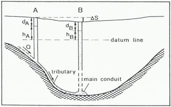
Fig. 7. Change of hydraulic head along a hypothetical tributary stream in the basal drainage system.
The drop in head along the tributary between sites A and Β is:
If a discharge ΔAQ is added through hole A, the depth of the water level changes by ΔdA, where ΔdA is less than zero for a rise in level. ΔdA consists of a part ΔdA , which accounts for the flow between sites A and B, and a part ΔdA,2 which accounts for the flow through hole A and its connnection to the tributary. Since the head varies approximately as the square of the discharge in the tributary

In the experiment, a discharge ΔQ = 0.065 m3min−1was pumped into hole A. The corresponding change in water level in the hole was ΔdA = −4 m.
A lower bound of the discharge Q through the tributary can be calculated if one assumes that ΔdA,2 was negligible (thus ΔdA,1 = −4 m) and that the water pressure in the main conduit was equal to the ice-overburden pressure. The ice depth at site Β is 2520 ± 20 m, and we assume a mean ice density of 915 ± 2kgm−3. The overburden pressure at site Β is thus equivalent to a water column of 2306 ± 7 m in height or dB = 214 ± 7m. In this case, by XS Equation (A1), Q = 0.746 ± 0.228 m3 min−1.
More likely, ΔdA,2 is not negligible and the water pressure in the main conduit is less than the ice-overburden pressure. For instance, assume that ΔdA,2 =ΔA,1 = −2m, and that d B = 274m. This gives Q = 5.36m3min−1. In any case, Q is much larger than ΔQ.
Appendix Β Vertical straining of ice within jakobshavns isbræ
This appendix presents a rough estimate of the strain field within Jakobshavns Isbræ upstream of the central borehole location. This appendix is intended to illustrate the idea that the vertical stretching at depth within the bedrock trough is larger than that in the near-surface ice, thus leading to an upward shift of the temperature minimum.
Consider the flow of ice in the zone of ice-stream convergence upstream of the borehole sites, as shown in Figure 8. Ice flows from section I to section II within a changing bedrock geometry. We assume that the flux of ice through the vertical faces AA’B’B and EE’D’D is zero. We make the additional assumption that the unknown bed profile along CD of the southern tributary is symmetrical with the bed profile along BC of the northern tributary, as indicated in Figure 8 by the dotted line. (No seismic soundings were made in this region.) Seismic data show the thickness of ice in the ice sheet above the trough is nearly constant ![]() .
.
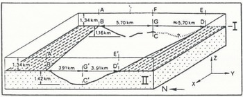
Fig. 8. Sketch of the confluence of Fakobshavns Isbræ based on seismic soundings along AF and A’E’ (T. Clarke and K. Echelmeyer, unpublished data). The depth of the ice stream is not known along CD; the dotted line is merely a mirror image of the bed along BC. In order to improve the clarity, the longitudinal scale has been chosen differently from the transverse one, with the actual distance between sections I and II being 5 km.
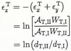
Ice is taken to be incompressible and the continuity relation is then used to relate the strain in the vertical direction z to that in two horizontal directions: x is longitudinal and y is transverse to the channel center line. Because the strains are large, we use the “natural” or logarithmic strain as defined by ϵ=ln(X f/X i) where X f and Χ i are the final and initial lengths in a given direction. All values are taken to be mean values for the cross-section unless noted otherwise. Superscripts S and Τ denote ice sheet and trough, respectively.
As a first approximation, we assume that there is no flux across the area BB’D’D. Because the thickness of the ice sheet is constant, there will be no vertical straining of the ice overlying the trough. Under this assumption, the strain field in the ice sheet can be assessed separately from that within the trough. Obviously, then, a parcel of ice traveling from section I to section II within the trough must extend in the vertical direction in accord with the increase in depth of the trough from I to II.
A quantitative analysis, based on continuity, is trivial in this example. However, we present it here because it is needed for the treatment of a different approximation later in this appendix. In detail, then we have.
i. Straining in the ice sheet above the trough
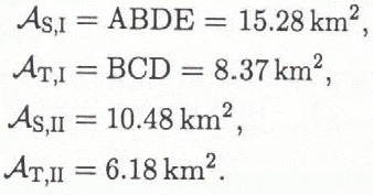
The transverse strain, ![]() corresponds to a reduction in width. At section II, the width of the ice sheet is W
s,u=A′E′=7.82km. At section I, the two tributaries join at an angle 2γ, and the width of each tributary must be measured perpendicular to the flow direction for flux considerations, hence W
S,I=AEcos γ, where AE=11.40 km and γ is not well known, but it is approximately 40°.
corresponds to a reduction in width. At section II, the width of the ice sheet is W
s,u=A′E′=7.82km. At section I, the two tributaries join at an angle 2γ, and the width of each tributary must be measured perpendicular to the flow direction for flux considerations, hence W
S,I=AEcos γ, where AE=11.40 km and γ is not well known, but it is approximately 40°.
Hence

The change in cross-sectional area As of the ice sheet will cause a longitudinal extension equal to

where ![]() . The vertical strain in the ice sheet is given by incompressibility, which, using Equations (B1) and (B2), yields
. The vertical strain in the ice sheet is given by incompressibility, which, using Equations (B1) and (B2), yields
as expected.
ii. Straining within the bedrock trough
Following a similar treatment of the change in trough dimensions,
where A T,I is the area within BCD and A T,ΙΙ is that within B’C’D’. The mean width of the channel is defined by
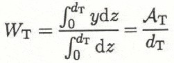
where d T is the maximum depth of the trough, as measured from the base of the ice sheet. The transverse strain is taken to be the change in this mean width from section I to II, as in Equation (B1).
From Equations (B4) and (B5), we have
as we would expect trivially from the earlier discussion. Given d
T,I = 1.16km and d
T,II = 1.42km, we find ![]() .
.
The assumption of no vertical straining in the ice sheet is perhaps somewhat unrealistic. An alternative assumption is that the longitudinal strain is independent of depth, or
which can be shown to be equivalent to the assumption that the longitudinal strain rate is proportional to the horizontal velocity. This is a reasonable assumption for sheet flow if the surface and bed slopes are small and if the shape of the velocity profile with depth does not vary significantly in the downstream direction. These conditions are not well satisfied in the present problem but an analysis of this case provides another, somewhat more realistic, scenario.
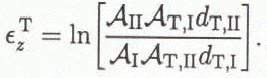
Under this model, εx is given by the change in total cross-sectional area A(= As + ΑT) from section I to II:
The mean transverse strains in the ice sheet and the trough are given in Equation (B1) and by the change in width, Equation (B5), respectively. Following Equation (B6), we have in the ice sheet

and, in the trough,
Numerical values are
Thus, following this assumption of uniform longitudinal strain, we obtain
and
which are similar in magnitude to the results obtained by assuming no vertical stretching in the ice sheet above the trough.
These results are only approximate in nature but they indicate that, near the zone of convergence, vertical straining along the center line is likely to be much larger at depth within the bedrock trough than near the surface. This depth variation will cause a distortion in the vertical temperature profile as it passes through the confluence. Consider, for example a parcel of ice starting at point G in Figure 8. The depth of this parcel is 1.34 km below the surface, which, using the maximum ice depth of 2.5 km in the northern tributary at section I, gives an initial relative depth of 0.54. When it arrives at section II, its depth below the surface is ![]() while the maximum total depth is 2.74 km there. Hence, its relative depth will have decreased to 0.50. This estimate is somewhat complicated by the bed geometry at section I, which shows that there is a rise in the bed directly below site G, and hence the relative depth of this parcel is actually closer to 0.68 at section I if the local ice depth FC is assumed. In any case, the relative depth for such a parcel of ice is distinctly less at section II than it is at section I.
while the maximum total depth is 2.74 km there. Hence, its relative depth will have decreased to 0.50. This estimate is somewhat complicated by the bed geometry at section I, which shows that there is a rise in the bed directly below site G, and hence the relative depth of this parcel is actually closer to 0.68 at section I if the local ice depth FC is assumed. In any case, the relative depth for such a parcel of ice is distinctly less at section II than it is at section I.
A remark regarding the first assumption stated above, in which no flux through the sides was allowed, and thus equal transverse convergence, is in order here. The convergence in the trough may well be stronger than that within the overlying ice sheet, since the latter is connected to the surrounding ice sheet. Allowing for stronger convergence in the trough would result in an even larger difference in vertical straining between trough and ice sheet.


