


1.Introduction
Laika ice cap (unofficial name) is a small icefield with a surface area of about 10 km2 on Coburg Island at the western edge of the North Water Polynya(Fig. 1). It extends from close to sea-level to an altitude of 530 m a.s.l., and has a highly negative mass balance with up to 2 m water-equivalent ablation per year in the lowest parts and only 0.3 m superimposed ice accumulation in a relatively small area at the top.
The ice cap rests on the relatively flat north-eastern side of an almost circular hill with steep rock walls extending down to the sea, except for three outlet valleys. The largest outlet glacier, Laika Glacier, merges towards the eastern side into a shore plain where it forms a piedmont-shaped tongue almost reaching sea-level. The second outlet, Wolf Glacier, is a steep glacier flowing down in a large couloir at the west side of the ice cap. A third valley trends in a south-east direction where a glacier, Icewall Glacier, terminates in a vertical ice wall about 40 m high.
In this study, three aspects of glaciological investigation are emphasized: (1) relations between the mass-balance pattern and the main meteorological factors such as precipitation, winds, and orography; (2) the recent and more long-term (100 years) changes of the glacier geometry; and (3) the thermal regime of Laika Glacier.
2.Investigations
Meteorology
During the North Water Project (Reference Müller, Ohmura and BraithwaiteMüller and others, 1977) from July 1972 to September 1976, continuous meteorological records at the Coburg Island base camp at 4 m a.s.l. and on the nearby Marina Mountain (Fig. 1) at 700 m a.s.l. were carried out. At both sites, automatic weather stations recorded temperature, humidity, and wind direction every 3 h together with the wind-run in the last 3 h. These records were completed with 6 hourly routine weather observations at the base camp with a continuously recording anemograph and an automatic precipitation gauge.
From August 1972 to August 1974, each component of the radiation balance was monitored.
The automatic weather station at both sites continued recording 3 hourly air temperatures until 1978. However, with only one or two maintenance services per year, these data are of lesser value for some seasons. In fall, rime formation on screen and sensors prevented measurements. The monthly mean values of air temperature may, however, still be usable.
Parallel to the shallow-depth ice-temperature measurements in the summer of 1975, in April a Stevenson screen with a thermohydrograph was installed on the top of Laika ice cap. This was run until the end of the measurements on 5 September. In July 1973, a radio-sonde program was initiated. Daily launches at 00.00 GMT up to the tropopause completed the meteorological investigations. These soundings continued until September 1974.
Glaciology
The glaciological investigations began with some ablation measurements on the Laika Glacier tongue in July 1973 by members of the North Water research project on Coburg Island. In 1974, these studies were continued with a minimum time investment in addition to the main meteorological investigations of the North Water Project. The emphasis on this study increased in 1975 after the completion of a thesis (Kappenberger, unpublished).
The mass balance is best documented for the period September 1974 to September 1975 with more than 200 snow-depth sounding sites, 15 snow-density pits, and about 50 ablation poles. The measurements were carried out several times between April 1975 and the end of the melt season in early September. Parallel to these measurements, qualitative maps of surface pollution by sand and dust, the number of days with ice ablation (snow-free ice surface or newly formed superimposed ice surface), and a geomorphological map with crevasses, ice structures, and melt-water rivers, were drawn. This information was used to interpolate between the balance measurements and to construct maps with winter, summer, and annual balance values (Fig. 2). Mass-balance studies were continued on a less intensive level until 1980 but, for most of these years, only the annual balance in the ablation zone proved to be usable.
A triangulation in the area surrounding the glacier gave the basis for drawing topographic maps. Aerial photographs taken in 1959 and 1971 were used to draw a map for the whole ice cap (1959) and again for the Laika Glacier tongue in 1971. The photogrammetric work was done using a Kern PG-2 stereo-plotting instrument. Additional aerial photographs taken in 1947 were not suitable for photogrammetric evaluation but could be used to determine the terminus for that year. For the period 1959–71, the surface lowering on the Laika Glacier tongue was mapped.
In the area around the narrow channel of Laika Glacier at about 200 m a.s.l., where the glacier tongue emerges from the ice cap, several stakes for the balance-study network and additional stakes in a transverse profile were surveyed a number of times between November 1973 and September 1976. These data were used to determine the annual mean and the seasonal fluctuation of the ice velocity.

Fig. 1. Maps of (a) the North Water area, (b) Coburg Island, and (c) Laika ice cap. The dashed line in map (a) denotes the fast-ice boundary in spring 1974. In map (b), the dotted line depicts the ice divide.

Fig. 2. Winter, summer, and annual mass-balance distribution on Laika ice cap for the year September 1974-August 1975. The map for the winter balance also shows the snow-pit sites (squares) and the snow-depth sounding locations (dots). The map for the summer balance shows the positions of the ablation stakes (circles), and the map for the annual balance shows the 100 m contours for the topography (dotted lines). All balance values are in cm water equivalent.
In the summer of 1975, a program for measuring englacial temperatures was carried out. On the top of the ice cap, a 10 m hole was drilled with a SIPRE corer and a multiple conductor cable with thermistors was inserted in early April. The hole was filled with snow and water. The temperatures came into equilibrium within 2 weeks and 17 measurements were made until 5 September. The core was used to determine the accumulation during previous years.
Five vertical holes were drilled to depths between 50 and 105 m, during the summer of 1975, along the center line of Laika Glacier from the highest point at 530 m a.s.l. down to the glacier tongue. The drilling with a hot-water jet has already been described (Reference Iken, Röthlisberger and HutterIken and others, 1977; Reference BlatterBlatter, 1985). Again, cables with thermistors were inserted into the holes and frozen in place. After adjustment of the temperatures, measurements were made and repeated in succeeding years.
3.Meteorology
General meteorology
Coburg Island has an Arctic maritime climate, as it is influenced by the effects of the nearby North Water Polynya (Ohmura and Müller, 1976) which produces stronger winds and higher precipitation than is normal in that latitude of the Canadian Arctic. In spite of the low elevation of the mountain tops (lower than 900 m), 60% of the island is glacier-covered. In order to discuss the causes of this ice distribution, some features of the local climate will be described.
The monthly means for the screen temperatures at the base camp are given in Table 1 together with the monthly means of the daily net radiation, cloud amount, daily range of the air temperature, and the amplitude of the periodic diurnal change of the screen temperatures for the 3 years September 1972-August 1975.
Table I. Climatological parameters measured at the coburg island base camp
The values are averages of 3 years (September 1972-August 1975) for the monthly means of the air temperature T, of the daily range R of the air temperatures, of the periodic diurnal amplitude A of the air temperature, and of the wind speed V. P denotes the monthly sum of the precipitation. The monthly mean of the daily sum of the global radiation G was measured from September 1972 to August 1974.

The difference between the annual mean air temperature at the base camp and on Marina Mountain is about 2.2°C. This is an annual mean lapse rate of only 0.3°C per 100 m. For the summer months of June, July, and August, the mean lapse rate is 0.5°C per 100 m, which is only slightly above the annual average. This small value can be explained by the cooling effect of the open-water surface around the island. The winter lapse rate is close to zero. The influence of the North Water Polynya and the open topography prevent stronger stable inversions during the winter months.
Coburg Island also shows a “Fram”-type seasonal change in diurnal amplitude of the air temperature, as is common for polar stations (Reference OhmuraOhmura, 1984). The monthly mean of the amplitude of the diurnal air-temperature variation reaches a maximum with 3°C in April and May, and decreases to 1.5°C in the summer months (Table 1).
An important factor for the mass balance of the glaciers on Coburg Island is the precipitation and the wind pattern. The wind statistics for the period September 1973 -September 1974 for all days and for days with precipitation above 2.5 mm w.e. are illustrated in Figure 3. These days account for 78% of the total precipitation in the period under consideration, and seem to play an important role in the glacier distribution on the island.

Fig. 3. Wind histogram for the Coburg Island base camp for the year September 1973-August 1974. The hollow bars denote the percentage of wind-run from the indicated direction. The densely shaded bars give the percentage of hours with wind from the indicated direction for days with more than 2.5 mm w.e. precipitation, and the widely shaded bars give the same for all days.
Precipitation usually occurs during the approach of a low-pressure system from the west and passing Coburg Island to the south. Under these conditions, precipitation is accompanied by moderate surface winds from the north to north-east, as is shown in the wind histogram (Fig. 3). The data from 12 radio-sonde ascents made during the time of precipitation show how the wind direction shifts from the north via the east to the south with increasing elevation. The largest fraction of precipitation is caused by the frontal lifting of air masses. Orographic lifting is minimal, not only because of the low height of the mountains on Coburg Island but also because the surface winds usually come from north to north-east during precipitation and shift to east or south-east at the altitude of the crests. Therefore, surface winds blow along the mountain range and only the air layers already at the elevation of the crest cross the island from east to west.
The strongest winds blow from the west. These winds are usually dry and occur after the passage of a precipitation region (mostly an occlusion) and the subsequent formation of an anticyclone in the west. This cold-air advection is chanelled through Jones Sound (Reference ItoIto, 1982) and is strengthened by the local polynya low-pressure system. This wind usually forms orographic stratocumulus with lenticular characteristics on the mountain chain. The strength and frequency occurrence of this wind is large enough to produce ventifacts. The vegetation in the windy region is sparse and is often restricted to small areas on the lee sides of the larger boulders (Müller, unpublished).
Snow-deposition pattern
On the north-western side of the prominent mountain chain of Coburg Island there are large glaciers that descend into the sea, whereas on the south-east side there are only a few glaciers in some of the valleys (Fig. 1b). This asymmetric glacier distribution system may be explained by several mechanisms: (1) the pattern of deposition of snow during precipitation may be influenced by prevailing wind situations and the orography; (2) the exposure and hence the radiation balance are correlated with the summer ablation; and (3) strong winds may erode the snow on exposed surfaces and thus not only reduce the winter accumulation but also increase the melt due to the resulting longer period of ice ablation. Some of the eroded snow is deposited on lee slopes with concave topography, thus increasing the accumulation.
The first and presumably the most important process is the deposition of snow in the upper parts of lee (north-west) slopes during precipitation. During a precipitation event, this snow drifts with the prevailing easterly winds at crest elevation and is thus deposited in the upper parts of the lee side (Reference FöhnFöhn, 1980; Reference Föhn and MeisterFöhn and Meister, 1983). This mechanism is confirmed by observations where slopes on both sides of ridges show different surface conditions. On Marina Mountain, a south-west-facing lee slope exhibits a firn surface at the end of the summer but the north-facing slope at the same altitude is already an ablation zone with an ice surface.
A second important reason for the asymmetry of the glacier distribution on Coburg Island lies in the exposure of the mountain slopes. The more heavily glacier-covered side is oriented north-west and hence receives less radiation and melt than the opposite south-east side.
The importance of the third reason, the west-wind situations, is more difficult to evaluate. The strong west wind coming from Jones Sound, which is covered by fast ice, causes considerable amounts of snow to drift in the lowest 20 m. During these situations, lenticular clouds were observed on the crest and on the lee (east) side of the island. This is an indication of a relatively stable layering of the lower troposphere during the approach of an anticyclone. The surface wind is therefore decelerated on approaching the island and must diverge around it to a considerable extent (personal communication from D. Grebner). Part of this air may also cross the island through the low passes (Fig. 4). The deceleration implies deposition of most of the drifted snow on the termini of the glaciers and this must also contribute to the accumulation. More snow also reduces the ice melt due to a longer period of snow ablation.

Fig. 4. Schematic orographic situation of Laika ice cap during west-wind situations. The arrows indicate the main surface wind ways through low-elevation passes and the fall winds. Along the profile P-P, locations with snow erosion (e) and with snow deposition (d) are marked. The 120 m [400 ft] topographic contours are broken on glacier-covered terrain. (JS Jones Sound, WG Wolf Glacier, LIC Laika ice cap. IG Icewall Glacier, Sc orographic stratocumulus, Ac lenticular altocumulus).
The air flowing across the island during these westerly storms descends very rapidly down the lee slopes and erodes the usually freshly fallen snow. This reduces the winter accumulation and increases the summer ablation on this side. This is confirmed by the observation that the snow depth on the south-east mountain side is small and only increases with greater distance from the foot of the mountains.
4.Mass Balance
Mass-balance pattern
The Laika ice cap is also exposed to the above-mentioned winds and precipitation events. To understand the observed balance pattern, the specific situation of the ice cap and its exposure to these processes must be taken into account. The orography mainly determines the accumulation pattern. However, the ablation could also be influenced by secondary effects. The smallest balance values occur at the snout of Wolf Glacier and on the orographic left side of the Laika Glacier tongue. As illustrated in Figure 4, these two sites are fully exposed to strong fall winds off the nearby mountains during westerly storms. Therefore, the winter balance is small since most of the snow is eroded and the two locations begin with ice ablation even at the commencement of the melt season (Fig. 2a). With the low altitudes of these locations, this resulted in net ablation of more than 2 m in the summer of 1975. Figure 5 illustrates the orographic situation of the Laika Glacier tongue.

Fig. 5. Oblique aerial photograph of the base camp (??) area with the Laika Glacier tongue (LG) in the center of the photograph. The large glacier valley in the background channels the westerly winds which erode the snow on the lower Laika Glacier tongue. The cliff of the Icewall Glacier (I) terminus is partly visible at the left side of the photograph. The snow patch (P) near the glacier outlet is a firn accumulation zone where snow is deposited during westerly storms. The photograph was taken on 22 August 1975, 2 d before the end of the ablation season.
The accumulation pattern observed on Laika ice cap can mostly be explained by two processes: (1) deposition of snow during precipitation events, and (2) deposition of wind-transported snow during and after snowfall.
Most precipitation falls during the summer season (Table 1). At higher elevations, part of the snow layer may become consolidated by rain or drizzle, which can form ice crusts preventing wind erosion and resulting in considerable accumulation. However, highest accumulations encountered on the ice cap are produced by orographic effects. As described in section 3, solid precipitation associated with wind produces additional accumulation on the higher parts of lee slopes. This is observed in the upper part of Wolf Glacier (Fig. 2a). Three other sites with high accumulation are due to drifted snow during westerly storms. These locations are near the top of Laika ice cap, on the orographic left side of Laika Glacier at 300 m a.s.l. (Fig. 5) and in the lowest part of Icewall Glacier (Fig. 2a). Part of the snow eroded by the fall wind in the valley west of the ice cap is drifted and deposited on these lee slopes with concave topography. On Icewall Glacier, the result is the largest firn accumulation encountered on the ice cap. These annual accumulation layers are clearly visible in the vertical ice cliff.
The topography around the Icewall Glacier terminus produces a rotor in the canyon-like valley which contributes to the shaping of the 40 m high cliff. The rotor axis is horizontal but perpendicular to the wind direction.
The ablation and accumulation processes discussed above have a greater influence on the balance values than the altitude. Therefore, it is not possible to determine a single representative equilibrium-line altitude for the ice cap and for Laika Glacier.

Fig. 6. Annual mass balance ai the stakes along the longitudinal profile of the Laika Glacier ablation zone. E denotes the elevation and b the mass balance in cm water equivalent.
History of the tongue of Laika Glacier
The piedmont-shaped tongue of Laika Glacier is retreating substantially over its entire terminus and the surface is lowering by as much as 2 m/year in some exposed areas. The total mass balance of the tongue can be defined by the mass loss from its surface and the influx of ice through the narrow channel at 200 m a.s.l. The surveyed surface velocity at the transverse profile was used to calculate the ice flow. The area of the channel profile was estimated by using a depth profile extrapolated from the surrounding topography and calibrated with the drill depth at site X2 (Fig. 1). The vertical profile of horizontal velocities was assumed to be a fourth-order parabola corresponding to Glen’s flow law with an exponent n = 3
and constant flow parameter A. This calculation yields 3.5 ± 0.7 × 10⁵ m3 ice per year flowing into the tongue, thus replacing only about 20% of the 1975 ablation. Although this ablation is about twice as high as the average, still less than half of the ablation is replaced by ice flow.
There is a trim line 20–30 m above the present glacier surface on the east side at about 150–200 m a.s.l. beside the narrow outlet (Fig. 7). This suggests that the glacier was previously one-third thicker at this place than it is today. Thus, the amount of ice that flowed through the outlet was possibly up to five times greater than today.
The reconstructed glacier termini for 1947, 1959, and 1971 are illustrated in Figure 7. Other features depicted show the limit of the glacier at its greatest extent during past centuries.
5.Thermal Regime
The measurements
The five bore holes for englacial temperature measurements are located along the center line of Laika Glacier. The profiles, measured in August 1975, are shown in Figure 8, together with an estimated two-dimensional temperature distribution in the longitudinal section. The measurements were repeated in succeeding years to confirm the equilibrium temperatures in the bore holes. The estimated accuracy is only ±0.2°C, although the calibration bath could be adjusted to 0.05°C. Under field conditions, this accuracy could apparently not be maintained.

Fig.7. Topographic map of the Laika Glacier tongue (situation 1971) together with contours of the surface lowering in the period 1959–71. The termini for 1947, 1959, and 1971 are outlined. TL denotes the trim line and M a moraine, both indicating the maximum extent during the last centuries. The arrows give measured surface velocities.

Fig.8.
Two-dimensional temperature distribution in the longitudinal profile of Laika Glacier. The measured vertical temperature profiles at all five sites are added to document the features discussed in section 5.
Near-surface temperatures
Along the profile with the five bore holes, exposure and slope do not vary much. Therefore, mean climatic conditions depend mainly on the elevation above sea-level and partly on the orographic situation. At the highest point, there is superimposed accumulation averaging 0.3 m/a. The drill site X4 lies a little above the average equilibrium line but in an area of maximum accumulation. X3 lies in the accumulation area in some extreme years. However, the 10 m temperatures show a strong dependence on the elevation (Fig. 9), indicating a strongly variable energy balance at different altitudes.
Especially remarkable are the 10 m temperatures at X4 with −6°C and at X3 with −4.5°C. This is around 9°C warmer than the annual mean air temperature and about 3–5°C warmer than the 10 m temperatures on the glacier tongue. The zone with a rapid change of near-surface ice temperatures lies between X5 and X4. Therefore, little information on the reason for this warming is available. There may be several reasons for this additional heat flux into the glacier, which partly may include: (I) an increased latent-heat flux due to superimposed ice formation; (2) a thick snow layer building up early in the fall insulates the glacier from the winter cold; and (3) freezing melt water captured in crevasses also releases latent heat in to the ice.

Fig. 9. m temperatures T along the longitudinal profile as a function of the elevation E.
The relative importance of each of these three possibilities is difficult to estimate. Point (1) can be true for X4 where the winter snow cover is up to 2 m thick and the net mass balance is at a maximum. However, X3 lies in the ablation zone for most years but the seasonal snow cover is also thick. Thus, the transient superimposed ice layer formed in the early part of the melt season may be considerable. On the other hand, the same can be said for X5, except that the superimposed ice layer mostly remains there. Point (2) is valid for all three sites X5, X4, and X3, but near-surface temperatures are much lower at X5. Point (3) is also difficult to evaluate. There is a crevassed zone around X4. Some of these crevasses were observed to remain partly water-filled at the end of the melt season. It is likely that part of this water refreezes in the crevasses and releases its latent heat into the ice. The early fall snow cover may help to store this heat in the ice. The average crevasse volume per unit area of ice surface was estimated by using aerial photographs. Around X4, an upper limit of this value is 0.25 m and, when the total volume of water refreezes in the crevasses, this contributes about 2.5 W m−2 as an annual average, compared with roughly 100 W m−2 of global radiation. On the other hand, the snow cover also prevents the opposite cooling effect due to cold air in open crevasses.
On the glacier tongue below 200 m a.s.l., the 10 m temperatures are again lower. Part of the surface often remains snow-free during the winter due to severe wind erosion. The lack of insulation by a snow layer exposes the ice more the winter cold.
The data are unsuitable for studying questions of energy balance in further detail except for the summit of the ice cap. The temperature profile in the top 10 m and in the snow layer (Fig. 10) with high temporal resolution during the 1975 summer allows a detailed interpretation. The temperature evolution in the top 10 m of the ice shows the propagation of the cold wave into the glacier. The velocity of propagation is about 30 m/a which is a factor of 1.5 too high for the annual wave in ice with a thermal diffusivity of 38m2/a. Since the annual temperature variation is not truly sinusoidal, this may be caused by harmonics with shorter periods. The warming in the snow layer during the early melt season appears to be more like a step function, which implies the fastest propagation of temperature variations into the ice (Reference Robin deRobin, 1970). The modelling of near-surface temperatures by Reference Greuell and OerlemansGreuell and Oerlemans (1987) produces a rather good fit to the observed temperature evolution.
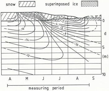
Fig.10. Temperature evolution in the top 10 m on the summit of Laika ice cap between April and September 1975.
Non-stationary temperatures
The top of Laika ice cap is an accumulation zone in today’s climate, though this cannot be certain for past decades with the relatively warm periods in the 1940s and 1950s. The vertical temperature profile at site X5 is convex with positive gradients decreasing with depth. For steady-state conditions with little influence of heat advection, this is only possible for upward-moving ice and thus in an ablation zone. There must be some non-stationarity in the measured profile.
The near-surface temperatures are determined by the energy balance at the surface. The only meteorological element for which reasonably reliable data for the last century exists is the air temperature. Annual means can be used for a first estimate of the surface-boundary condition in order to discuss the shape of the measured vertical profile X5.
The time series of Arctic (lat. 65–85°N.) annual mean air temperatures (Reference JonesJones, 1985) suggests a roughly sinusoidal temperature variation with a roughly 80 year period (Fig. 11). Minimum temperatures occurred at about 1890 and 1970. The amplitude of this spatially averaged variation is ±0.8°C, which seems to be small when compared with the temperature variation recorded at the Upernavik, West Greenland, meteorological station (Fig. 11).
Site X5 is located on the top of the ice cap. There are no measurements of the horizontal ice movement. Considering the small ice thickness and the horizontal ice surface, this velocity must be very small. Since most factors like the geothermal heat flux and the recent history of mass balance and ice thickness are unknown, a one-dimensional but time-dependent model is adequate for calculating the temperature profile. All values for ice qualities, mass balance, ice thickness, and bottom-temperature gradient are assumed constant, and only the surface temperature is allowed to vary with time.

Fig.11. Long-term series of the annual mean air temperatures at Upernavik (U), West Greenland, and for the Arctic (A) (lat. 65°-85° N.). The two series have been smoothed with a 13 point binomial filter.
For a one-dimensional, non-stationary model with a sinusoidal surface-temperature variation and a vertical ice velocity which is proportional to the distance to the glacier bed, an analytical solution is possible. The temperature profile is governed by the equation
The z -axis points downward and z = 0 at the glacier surface, and h is the glacier thickness. With a surface-boundary condition
the solution for the periodic part is
with the amplitude

and the phase shift


This is a partial solution of Equation (1) leaving aside transient and stationary parts. Surprisingly, the phase shift a only depends on even powers of the velocity v. The stationary part of the solution of Equation (1) is given by

where y = h − Z. θb and (dθ/dZ)b are the bottom temperature and bottom-temperature gradient, respectively. With a linear velocity profile

this solution corresponds to the solution given by Reference PatersonPaterson (1981):

with ![]() . Figure 10 shows solutions for a steady-state profile θs(Z) and a situation θ(z,t)= θ s(z) + θp(z,t) for the time-dependent model with the values for boundary conditions and constants as given in the caption of Figure 12. The calculated profile (n) fits the data quite well. The comparison between possible steady-state scenarios and the measured profile strongly suggests a temporal variation of the surface-boundary condition, mostly a cooling during the previous three to four decades.
. Figure 10 shows solutions for a steady-state profile θs(Z) and a situation θ(z,t)= θ s(z) + θp(z,t) for the time-dependent model with the values for boundary conditions and constants as given in the caption of Figure 12. The calculated profile (n) fits the data quite well. The comparison between possible steady-state scenarios and the measured profile strongly suggests a temporal variation of the surface-boundary condition, mostly a cooling during the previous three to four decades.
For the small vertical velocities derived from the accumulation rate of superimposed ice, a much simpler calculation taking a static ice body produces very similar temperature profiles. A more sophisticated model than the one described above is inadequate with present knowledge of the history of the ice cap. The variations of the mass balance and the related energy balance, and hence surface temperature, cannot be reconstructed with the available data. Furthermore, the past and present patterns of the geothermal conditions must be very complicated for this mountainous island with changing glaciation.

Fig.12. Calculated and measured temperature profiles at site X5. The boundary conditions for the stationary profile (s) are θ0 = −9.3°C and the bottom gradient (d θ/dz)b = 0.02° C/m. The vertical component of the velocity at the surface is 0.3 m/a. the ice thickness is 50 m, and the thermal diffusivity k = 38 m2/a. The sinusoidal surface-temperature variations are chosen to vary with an amplitude of ±2.2°C and a period of 80 years. The non-stationary profile is calculated for the moment of minimum surface temperature at t = 60 a.
Basal temperatures
Most of the bed of Laika ice cap is cold. Especially in the accumulation zone, basal temperatures are as low as −10°C Seasonal surface-velocity fluctuations indicate an area of temperate basal ice in the ablation zone. The temperate region is surrounded by a cold-ice ring. This pattern has been reported for many other cold valley glaciers or ice caps (Reference SchyttSchytt, 1969; Reference Classen and ClarkeClassen and Clarke, 1971; Reference Clarke and GoodmanClarke and Goodman, 1975; Reference Jarvis and ClarkeJarvis and Clarke, 1975; Reference ClarkeClarke, 1976; Reference Clarke and JarvisClarke and Jarvis, 1976; Reference ClassenClassen, 1977; Reference BlatterBlatter, 1987).
On Laika Glacier, the vertical temperature profiles in the tongue area (X2 and X3) show a vanishing temperature gradient near the glacier bed (Fig. 8). At bore hole X2, the lowest five thermistors, covering a layer 25 m in thickness, remained at the same temperature as was recorded immediately after their insertion into the water-filled bore hole. This suggests the possibility of a thick layer of temperate ice and an internal phase boundary. Similar observations were reported by Classen (1977) for the surge zone of the Barnes Ice Cap, Baffin Island, Canada, and by Reference Stauffer and OeschgerStauffer and Oeschger (1979) for the EGIG Camp III near the edge of the Greenland ice sheet. Blatter (Reference Blatter1985, 1987) found the same feature in White Glacier, Axel Heiberg Island, N.W.T., Canada. In most cases, the temperature measurements were not sufficiently accurate to be certain of the existence of an internal phase boundary. However, core drilling in Greenland was made more difficult by the fact that the wet core had to be lifted through cold ice. Radio echo-sounding done on sub-polar glaciers in Svalbard revealed internal reflecting layers which are related to temperate zones below cold near-surface layers (Reference BamberBamber, 1987; Reference Kotlyakov and MacheretKotlyakov and Macheret, 1987). A mathematical model for handling the thermal regime of this type of polythermal glacier has been prepared and the results will be published in a forthcoming paper.
6.Conclusions and Prospects
Conclusions
Three features observed on Laika ice cap emphasize the complexity of glacier-climate relations. The first problem is related to mass-balance patterns, the second to near-surface temperatures and non-stationarity, and the third to internal phase boundaries making glaciers polythermal.
Laika ice cap is situated in an Arctic climate which is maritime due to the nearby North Water Polynya but which is also determined by the strong westerly winds channelled through Jones Sound. Therefore, the influence of the orography on the mass-balance distribution is substantially increased. This also questions such approaches of parameterizing balance features such as equilibrium-line altitudes with single climatological elements like air temperature. Re-distribution of snow by wind drift may result in the same amount as the direct deposition of solid precipitation. This is especially true for small glaciers. The orography gains in importance as the horizontal extent approaches the order of magnitude of the topographic elevation range. Even the usual pattern of increasing balance may temporarily become reversed. The largest accumulation on Icewall Glacier occurs at the glacier terminus. The ablation distribution shows smoother patterns than those for accumulation. Altitude and exposure mostly determine the melt. However, large snow accumulation indirectly decreases the melt rate due to longer snow ablation.
Non-stationary climatic conditions lead to non-stationary englacial temperatures. Time-scales for dynamic processes are very different for large polar ice caps and for valley glaciers. When large ice sheets react to long-term climatic changes like ice ages and interstadials, they never reach a steady state (Reference Jenssen and RadokJenssen and Radok, 1961, 1963). The same is true for glaciers where time-scales for geometric changes and for changes of internal temperatures are of the order of decades and centuries. If these changes are forced by climatic variations of similar periodicities, glaciers can never reach a steady state either. Considering the wide spectrum of more or less periodic climatic variations, this is likely to be the general situation.
The thermal regime of Laika Glacier shows an extended layer of temperate basal ice with an internal phase boundary in the ablation zone. The question arises whether this is a common feature for many cold valley or outlet glaciers. At present, the existence of such internal phase boundaries can only be established by accurate measurements.
Prospects
The small size and the relatively simple geometry of Laika ice cap make it suitable for detailed studies of thermal and dynamic inter-relations. Future field studies will concentrate on the near-surface temperatures and the energy balance around the mean equilibrium-line altitude, and on an accurate location of the internal cold-temperate transition surface, either by radar sounding or by accurate temperature measurements. On the theoretical side, a model for calculating the thermomechanics of a polythermal glacier tongue is now being developed in addition to simpler thermal or dynamic models for discussing measured temperature profiles.
Acknowledgements
The field studies on Laika ice cap were made possible by the generous logistic and financial support of the Polar Continental Shelf Project, Ottawa, Canada, and the Swiss Federal Institute of Technology, Zürich. Professor A. Ohmura supported this study in many important aspects and through fruitful discussions. The authors wish to thank Dr A. Iken, Dr N. Deichmann, and M. Kappenberger for their reliable work on the glacier and their friendship during the field seasons. Dr G. Holdsworth and Dr M. M. Brugman read the manuscript and helped to improve it substantially. Dr D. Grebner gave valuable information on meteorological matters. The authors wish to thank the anonymous reviewers who encouraged a major revision and completion of the first draft.


