


1. Introduction
Studies of temperate and predominantly warm polythermal glaciers (polythermal structure types b and c of Reference Blatter and HutterBlatter and Hutter, 1991, fig. 1) have clearly demonstrated that there is an intricate coupling between the subglacial hydrology and flow dynamics of such glaciers (Reference IkenIken,1981; Reference BindschadlerBindschadler, 1983; Reference Iken, Röthlisberger, Flotron and HaeberliIken and others, 1983; Reference Iken and BindschadlerIken and Bindschadler, 1986; Reference KambKamb, 1987; Reference JanssonJansson, 1995, Reference Jansson1996; Reference Raymond, Benedict, Harrison, Echelmeyer and SturmRaymond and others, 1995; Reference Harbor, Sharp, Copland, Hubbard, Nienow and MairHarbor and others, 1997; Reference Kavanaugh and ClarkeKavanaugh and Clarke, 2001; Reference Mair, Nienow, Willis and SharpMair and others, 2001, Reference Mair, Sharp and Willis2002).This coupling is especially important when surface meltwater is able to penetrate to the glacier bed, and it is fundamental to such dynamic phenomena as glacier surges, seasonal velocity variations and short-term high-velocity events. Whether and how this coupling affects the dynamics of glaciers composed predominantly of ice at sub-freezing temperatures is less clear. The goal of this paper is therefore to investigate the relationships between surface melt, subglacial hydrology and the flow of a predominantly cold polythermal glacier in the Canadian High Arctic.
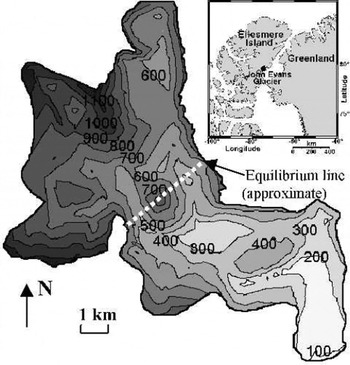
Fig. 1. Bed topography (m a.s.l.) and location of John Evans Glacier.
Predominantly cold polythermal glaciers (polythermal structure types d and e of Reference Blatter and HutterBlatter and Hutter, 1991, fig. 1) are characterized by a thick mantle of cold ice overlying a limited area of temperate ice at, and immediately above, the glacier bed in the ablation area. Examples include White Glacier, Axel Heiberg Island, Canada (Reference BlatterBlatter, 1987), and McCall Glacier, Alaska, U.S.A. (Reference Rabus and EchelmeyerRabus and Echelmeyer,1997). A recent review (Reference HodgkinsHodgkins, 1997) suggests that penetration of surface-derived meltwaters to the beds of such glaciers is limited. This is because: (a) water flow along intergranular vein networks is largely absent in cold ice, and (b) crevasses and moulins, which introduce large-scale permeability to glacier ice, are rare on predominantly cold glaciers due to low rates of ice deformation and the refreezing of meltwater that drains into crevasses. If this were the case, the influence of surface melting on the flow of predominantly cold polythermal glaciers would be limited.
Several studies, however, suggest that the surface velocities of such glaciers vary on a seasonal basis (Reference Müller and IkenMüller and Iken,1973; Reference IkenIken,1974; Reference AndreasenAndreasen,1985; Reference Rabus and EchelmeyerRabus and Echelmeyer, 1997). This is also the case on the Greenland ice sheet, where melt-induced seasonal variations in surface velocity have been observed in a region where cold ice is >1200 m thick (Reference Zwally, Abdalati, Herring, Larson, Saba and SteffenZwally and others, 2002). These studies imply that surface meltwaters can and do penetrate to the glacier bed through significant thicknesses of ice at sub-freezing temperatures, contrary to the suggestion of Reference HodgkinsHodgkins (1997). They also suggest that coupling between surface melting and the flow of predominantly cold, but warm-based, ice masses may provide a mechanism by which such ice masses can respond rapidly to changes in surface weather and climate (Reference Zwally, Abdalati, Herring, Larson, Saba and SteffenZwally and others, 2002). Given model predictions that anthropogenic climate warming will be most marked in northern high latitudes (Reference Manabe, Stouffer, Spelman and BryanManabe and others, 1991), and the potential contribution of Arctic glaciers to global sea level, understanding of this coupling is a high scientific priority.
1.1. Study site
The study was conducted at John Evans Glacier, a ∼165 km2 predominantly cold polythermal valley glacier on the east coast of Ellesmere Island, Nunavut, Canada (79°40′ N, 74°30′ W; Fig. 1). The glacier ranges in elevation from 100 to 1500 m a.s.l., with the long-term equilibrium line at ∼750–850 m a.s.l. Ice depths reach a maximum of 400 m in the upper ablation area, and average 100–250 m in the lower ablation area where the velocity measurements were made (Reference Copland and SharpCopland and Sharp,2001). For the period 1997–99,the mean annual air temperature at 820 m a.s.l. was −15.2°C.
High bed reflection powers in radio-echo sounding records indicate warm ice at the bed throughout most of the lower ablation zone, except along the glacier margins and where the ice is thin (Reference Copland and SharpCopland and Sharp, 2001). A continuous internal reflecting horizon over the centre of the lower terminus suggests that the warm basal ice reaches an average thickness of 20 m there. In the accumulation and upper ablation areas, low bed reflection powers and 15 m borehole temperatures of −9.5 to −15.1°C suggest that the ice is cold throughout.
The melt season typically occurs between earlyJune and early August. At the start of the melt season, meltwater either ponds on the glacier surface or is routed directly to the ice margins, and is unable to access the glacier interior. Once englacial drainage of supraglacially derived meltwaters is initiated, however, approximately 25% of the glacier surface area drains into moulins in a crevasse field at the top of the terminus (Fig. 2). Later in the melt season, meltwater from up to 40% of the surface area of the glacier drains to the glacier bed via these moulins and a second crevasse field ∼6 km further upstream. Dye tracer experiments confirm the link between these water input locations and a major drainage portal at the terminus (Reference Bingham, Nienow and SharpBingham and others, 2003). Large increases in the suspended-sediment content and electrical conductivity (EC) of the water as it passes through the glacier suggest that it is routed subglacially (Reference Skidmore and SharpSkidmore and Sharp,1999).

Fig. 2. Landsat 7 image of John Evans Glacier (path 049, row 002, 10 July 1999) showing the location of the velocity stakes (black dots), geophones (white dots; LG = lower geophone, MG = middle geophone, UG = upper geophone), surveying base stations (white squares), stream gauging stations (triangles) and artesian fountain observed in 1998 (x). Crevasse field indicates location where most supraglacial meltwater reaches the glacier bed. Lower weather station is located next to the middle geophone. Black box indicates horizontal extent of Figures 4 and 7.
In the early summer, the meltwater is trapped at the glacier bed behind the frozen terminus (Reference Skidmore and SharpSkidmore and Sharp, 1999). The initial release of subglacially routed meltwater from the glacier typically occurs via an artesian fountain on the glacier surface (Fig. 3) and/or upwelling through sediments a few metres in front of the snout. Since observations began in 1994, dates of initiation of subglacial outflow have varied between 22 June and 11 July (days 173–192). As outflow continues, the upwelling migrates towards the snout, and is eventually replaced by the formation of an ice-walled channel at the glacier bed (the major drainage portal referred to in the previous paragraph). The first water to be released has high total solute concentrations (EC > 300 μs cm−1), is somewhat turbid and, relative to supraglacial runoff, contains elevated concentrations of ionic species (Na+ , K+ and Si) that are products of silicate weathering (Reference Skidmore and SharpSkidmore and Sharp, 1999). Within a few days, the water becomes more dilute, although solute concentrations are still much higher (>100 μs cm−1) than for supraglacial water (<10 μs cm−1). These observations suggest that the first water to be released has been stored for a long period (possibly over winter), while later waters have been transmitted more rapidly through the englacial and subglacial drainage system.
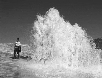
Fig. 3. Artesian fountain observed on the lower terminus between days 180 and 186, 1998; see Figure 2 for location.
2. Measurements
2.1. Surface velocity
Twenty-one velocity stakes were established over the lower-most 2 km of John Evans Glacier in 1998. An additional 13 stakes were added in 1999 to extend the network 1 km further up-glacier (Fig. 2). The terminus region was chosen for study as it is easily accessible, there are surrounding cliffs that allow survey stations to be located on bedrock, and subglacial water flow appears to be present (Reference Skidmore and SharpSkidmore and Sharp, 1999; Reference Copland and SharpCopland and Sharp, 2001). Reflecting prisms were mounted on 3 m long stakes drilled and subsequently frozen into the ice surface. These were periodically redrilled or replaced before surface melting made them unstable.
The position of each prism was measured daily (weather permitting) in the summers of 1998 and 1999 with a Geodimeter 540 total station theodolite. To reduce errors, the data were subsampled to determine stake displacements over periods of 2 days or longer. The time between surveys was used to convert the displacements to velocities in cm d−1 (24 hours). Velocity patterns were interpolated over the entire terminus region from the point measurements at the stakes.Velocities were set to 0 around the glacier edge, which is reasonable given that the glacier appears to be frozen to its bed at the margins (Reference Copland and SharpCopland and Sharp, 2001). All interpolations were completed with the “v4” interpolation routine in Matlab, which is based on biharmonic spline interpolation (Reference SandwellSandwell, 1987). Interpretations of velocity patterns are made only for areas where stakes are present. For the purposes of our discussion, the lower terminus is defined as the area south of the upper geophone (UG in Fig. 2), and the upper terminus is defined as the area to the north and northwest of this geophone.
2.2. Surface velocity errors
From the Geodimeter technical specifications, uncertainties in distance measurements amount to ± (2 mm + 3 ppm). This equates to ±5 mm over a typical survey distance of 1 km. Angle measurements were made to a resolution of 2″, which equates to a maximum potential error of ±4.8 mm over a distance of 1 km. Instrument drift during surveys was corrected for by resurveying the position of reference markers after every seven or fewer stake measurements and assuming that drift was linear between surveys. In the following discussion, three types of error are evaluated:
-
(i) Position error (± cm): this is the error in determining the location of a stake during a single survey.
-
(ii) Displacement error (± cm): this is the error in determining the displacement of a stake between two surveys. It is calculated by summing the position errors from the two surveys and/or from two or more independent measurements of the displacement of a stake.
-
(iii) Velocity error (± cm d−1): this is the displacement error adjusted for the time between surveys. As the measurement period increases, the velocity error decreases as the displacement error is divided by a greater time interval.
In 1998, all stakes were surveyed independently from each of two stations located ∼100 m apart. For each measurement period, this provided two measures of the displacement of each stake, and the displacement error was calculated from the difference between these and the mean displacement of the stake for that survey. Separate velocity error calculations were then made for each stake for each 2 day measurement period. These are displayed in the velocity figures discussed later. For the entire 1998 measurement period, mean errors for all stakes are ±1.1 cm d−1 in horizontal velocity and ±0.6 cm d−1 in vertical velocity.
In 1999, the displacement of each stake was determined once for each measurement period from surveys at a single station. To evaluate errors, the location of each stake was measured at least twice from the same station during each survey in July and August. On a given day, the difference between the two or more measurements of a stake and its mean location provides a position error. The position errors from the surveys at the start and end of a measurement period then provide the displacement error, which in turn provides the velocity error. The velocity errors were calculated separately for each stake for each 2 day measurement period. For summer 1999, the mean errors for all stakes were ±0.6 cm d−1 in horizontal velocity and ±0.2 cm d−1 in vertical velocity.
The following discussions focus mainly on the 1999 measurements due to the lower velocity errors, improved spatial coverage, and better records from supporting instruments. In these discussions, the stated start and end times of velocity “events” are approximate due to the 2 day resolution of the measurements. This likely leads to underestimation of the true magnitude of velocity changes since events will likely span more than one measurement period, or be shorter than a measurement period.
2.3. Geophones
In 1997, three geophones were installed at 5 m depth along the centre of the terminus: a lower geophone ∼0.3 km up-glacier from the snout, a middle geophone ∼1 km from the snout, and an upper geophone ∼2 km from the snout (Fig. 2). The 4.5 Hz geophones were interfaced to a Campbell Scientific data logger, which counted the number of seismic events above a defined threshold and output a total every hour (in 1998) or 2 hours (in 1999). Geophone sensitivity was adjusted to a level that provided a good compromise between sensitivity and noise rejection in studies at Trapridge Glacier, Canada (Reference Kavanaugh and ClarkeKavanaugh and Clarke, 2001). The geophone records did not allow for accurate location of individual seismic events because it was not possible to distinguish a weak local event from a strong distant one, although it was possible to determine general positioning by noting which geophones recorded activity.
Given the lack of volcanic activity and of active faults in this area, it is assumed that most detected events had a glacial origin. Previous studies at other glaciers have shown strong correlations between ice velocity, water discharge and seismicity (Reference Iken and BindschadlerIken and Bindschadler, 1986; Reference Raymond, Benedict, Harrison, Echelmeyer and SturmRaymond and others, 1995; Reference Kavanaugh and ClarkeKavanaugh and Clarke, 2001). This is because ice fracturing commonly occurs during periods of rapid ice velocity due to changes in the internal stress distribution. In addition, basal sliding may produce seismic events as the ice moves across the glacier bed.
2.4. Weather stations
Three automatic weather stations were installed on John Evans Glacier in May 1996.The lower station is located next to the middle geophone in the centre of the terminus at ∼200 m a.s.l. (Fig. 2). Hourly measurements of air temperature and surface albedo from this station were used to quantify changes in weather and ice surface conditions. Rates of surface lowering recorded by an ultrasonic depth gauge (UDG) provide an indication of relative rates of meltwater production. These records have not been corrected for differences in surface density between ice and snow, so provide only a general measure of surface melt rates.
2.5. Discharge records
To provide an indication of the meltwater inputs to the subglacial drainage system in 1999, pressure sensors were installed upstream of the main crevasse field in an ice-marginal lake and at two locations in a supraglacial stream draining from the lake (Fig. 2). To monitor the flow of water from the glacier, a pressure sensor was installed in the main subglacial stream shortly after it exited the snout. This proglacial record is approximate due to frequent bed aggradation and erosion around the sensor and the need to move the sensor because of channel migration. The sensors were not calibrated to discharge, so each record was rendered dimensionless by scaling it between the highest and lowest water levels over the period of interest.
2.6. Subglacial flow routing
Reference Copland and SharpCopland and Sharp (2000) reconstructed subglacial flow routing at John Evans Glacier from the form of the subglacial hydraulic potential surface using the method of Reference ShreveShreve (1972). Reconstructions were made for assumed basal water pressures at 0–100% of ice overburden pressure, but no significant differences were found in predicted flow routing. This indicates that subglacial topography, rather than variations in ice thickness, provides the dominant control on basal water flow at John Evans Glacier.The drainagepattern presented here is for basal water pressures at 100% of ice overburden pressure.
2.7. Residual vertical velocity (cavity opening)
To determine the importance of basal processes in accounting for the measured vertical velocities, the residual vertical velocity (w c) was calculated for each survey. This is the vertical velocity remaining after vertical strain and the horizontal movement along a sloping bed have been accounted for, and is commonly attributed to basal cavity formation (Reference Iken, Röthlisberger, Flotron and HaeberliIken and others, 1983; Reference Hooke, Calla, Holmlund, Nilsson and StroevenHooke and others, 1989). In reality, it may be caused by any unaccounted-for basal process, such as a change in the dilatancy of subglacial till. w c was calculated from (Reference Hooke, Calla, Holmlund, Nilsson and StroevenHooke and others, 1989):
where w
s is measured Lagrangian vertical velocity at the surface, u
b is horizontal basal velocity, β is bed slope,
![]() is depth-averaged vertical strain rate, and h is ice thickness. For these calculations, measured values of u
s (horizontal surface velocity) interpolated to a regular 100 m grid were used instead of u
b, since basal velocity was not measured directly. Since u
b ≤ u
s, in general, this will produce a minimum estimate of the rate of cavity opening. Ice thickness was determined by radio-echo sounding (Reference Copland and SharpCopland and Sharp, 2001), and interpolated to the same 100 m grid. Bed slope was calculated from the change in bed elevation across the four gridpoints to the north, east, south and west of the point of interest.
is depth-averaged vertical strain rate, and h is ice thickness. For these calculations, measured values of u
s (horizontal surface velocity) interpolated to a regular 100 m grid were used instead of u
b, since basal velocity was not measured directly. Since u
b ≤ u
s, in general, this will produce a minimum estimate of the rate of cavity opening. Ice thickness was determined by radio-echo sounding (Reference Copland and SharpCopland and Sharp, 2001), and interpolated to the same 100 m grid. Bed slope was calculated from the change in bed elevation across the four gridpoints to the north, east, south and west of the point of interest.
In Equation (1),
![]() (the measured vertical strain rate at the surface) was initially used as an approximation to
(the measured vertical strain rate at the surface) was initially used as an approximation to
![]() . By assuming incompressibility,
. By assuming incompressibility,
![]() was determined from the surface horizontal strain rates
was determined from the surface horizontal strain rates
![]() , which were calculated from the gradients in surface horizontal velocity between adjacent gridpoints. In reality,
, which were calculated from the gradients in surface horizontal velocity between adjacent gridpoints. In reality,
![]() is unlikely to be the same as
is unlikely to be the same as
![]() at depth (Reference Balise and RaymondBalise and Raymond, 1985; Reference Hooke, Calla, Holmlund, Nilsson and StroevenHooke and others, 1989), so it is necessary to assess how vertical variations in
at depth (Reference Balise and RaymondBalise and Raymond, 1985; Reference Hooke, Calla, Holmlund, Nilsson and StroevenHooke and others, 1989), so it is necessary to assess how vertical variations in
![]() would affect calculations of w
c.
would affect calculations of w
c.
If it is assumed that there is no cavity opening (w
c = 0), and that 0 < u
b < u
s, then for a given ice thickness it is possible to determine whether and how
![]() must vary with depth (Reference Hooke, Calla, Holmlund, Nilsson and StroevenHooke and others, 1989; Reference Mair, Sharp and WillisMair and others, 2002). For negative values of β (i.e. when the glacier is flowing down-hill), three cases are possible:
must vary with depth (Reference Hooke, Calla, Holmlund, Nilsson and StroevenHooke and others, 1989; Reference Mair, Sharp and WillisMair and others, 2002). For negative values of β (i.e. when the glacier is flowing down-hill), three cases are possible:
-
(a)
 is not required to change with depth relative to
-
(b)
is required to decrease with depth relative to
-
(c)
is required to increase with depth relative to
.
These equations are reversed in the more unusual case when β is positive (i.e. when the glacier is flowing uphill). Basal vertical displacement is unlikely to have occurred if the surface vertical velocity can be explained by a combination of basal sliding and vertical strain rates that are either constant or decreasing with depth (i.e. scenarios a and b above). Basal vertical displacement is most likely to have occurred if the surface vertical velocity is higher than can be plausibly explained by an increase in
![]() with depth relative to
with depth relative to
![]() (scenario c above). Classification of the glacier into areas where each of these cases holds for each velocity event therefore helps in defining areas where basal vertical displacement is likely to have occurred. Reference Hooke, Calla, Holmlund, Nilsson and StroevenHooke and others (1989) argued that a value of
(scenario c above). Classification of the glacier into areas where each of these cases holds for each velocity event therefore helps in defining areas where basal vertical displacement is likely to have occurred. Reference Hooke, Calla, Holmlund, Nilsson and StroevenHooke and others (1989) argued that a value of
![]() that is ∼3 mm d−1 less than w
s (when β is negative) is likely indicative of cavity opening under ice ∼100 m thick. To ensure that areas of basal vertical displacement are conservatively identified at John Evans Glacier, discussion is limited to areas where the inferred rate of cavity opening is at least 1 cm d−1.
that is ∼3 mm d−1 less than w
s (when β is negative) is likely indicative of cavity opening under ice ∼100 m thick. To ensure that areas of basal vertical displacement are conservatively identified at John Evans Glacier, discussion is limited to areas where the inferred rate of cavity opening is at least 1 cm d−1.
3. Results
3.1. Long-term velocities
Velocities were calculated for winter 1998/99 (day 205,1998 to day 146, 1999) and 1999/2000 (day 214, 1999 to day 161, 2000) to provide a measure of the “background” velocities against which short-term variations can be compared. Only the winter 1999/2000 velocities are presented here, as the records cover a larger area and are very similar to the 1998/99 records (Fig. 4). For the stakes that were measured in both winters, differences average 0.14 cm d−1 in horizontal velocity and 0.57° in horizontal direction.

Fig. 4. (a) Winter 1999/2000 horizontal velocity contours. Each arrow indicates the direction and velocity of a stake. Squares indicate stakes grouped into factor 1 in principal component analysis (PCA; see end of section 3.1 for explanation); circles indicate stakes grouped into factor 2. (b) Winter 1999/ 2000 vertical velocity contours. All velocities in cm d−1
The mean horizontal velocity for all stakes was 3.5 cm d−1 for winter 1999/2000, compared to a mean horizontal velocity of 5.3 cm d−1 for summer 1999 (days 175.50–204.88,1999) (Fig. 5). Horizontal velocities for summer 1998 were also ∼50% higher than winter values, which suggests that basal sliding is an important process during at least the summer at John Evans Glacier. This seasonal increase in horizontal velocity is not distributed evenly, however, but is concentrated during 2–4 day high-velocity events, which provide the focus of the discussion below. Vertical velocities are low during the winter, reaching a maximum of approximately −0.5 cm d−1 in an area of steep surface slopes between the upper and lower terminus (Fig. 4b). Mean vertical velocities generally vary little between winter and summer, although significant variations do occur during some high-horizontal-velocity events (Fig. 6).
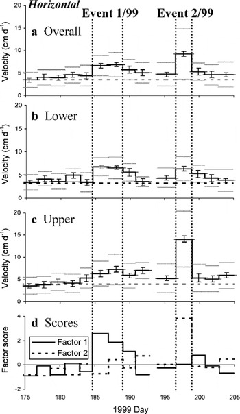
Fig. 5. Summer 1999 mean horizontal velocities (solid black line), winter 1999/2000 mean horizontal velocities (dashed line), errors in horizontal velocity (vertical bars), and standard deviation in horizontal velocity (grey lines): (a) for all stakes; (b) for stakes grouped by factor 1 in PCA (i.e. lower terminus); and (c) for stakes grouped by factor 2 in PCA (i.e. upper terminus). (d) Factor scores for the two factors (i.e. the standardized PCA scores on the factors over the measurement period).
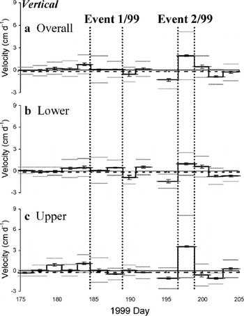
Fig. 6. Summer 1999 mean vertical velocities (solid black line), winter 1999/2000 mean vertical velocities (dashed line), errors in vertical velocity (vertical bars), and standard deviation in vertical velocity (grey lines): (a) for all stakes; (b) for stakes grouped by factor 1 in PCA (i.e. lower terminus); and (c) for stakes grouped by factor 2 in PCA (i.e. upper terminus).
To assess the spatial scale of forcing mechanisms and how these change over time, principal component analysis (PCA) was used to define groups of stakes with coherent patterns of horizontal velocity variation (Reference JohnstonJohnston, 1978). From analysis of all 2 day horizontal velocity data over days 164.71–211.98, 1999, PCA identified eight principal component factors with eigenvalues >1 (Table 1). When the 34 velocity stakes are grouped based on their loadings on these factors, two main clusters are identified: factor 1 groups stakes from the lower terminus, while factor 2 groups stakes from the upper terminus (Fig. 4a). Grouping using more than the first two factors subdivides these two clusters into smaller groups that are not as spatially contiguous. In addition, the percentage of variance explained by the other factors is generally low (Table 1). Since most of the variance in horizontal velocity is explained by the first two factors (63.9%), and the loadings on these factors cluster stakes into populations that act differently during high-velocity events (see below and Fig. 5d), these groupings are used in discussion of the 1999 short-term velocity data. PCA was not performed on the 1998 velocity data due to the relatively small number of stakes in that year.
Table 1. Eigenvalues and explained variance for the principal component factors with an eigenvalue >1 from a PCA of 2 day horizontal velocities over days164.71–211.98, 1999
3.2. 1999 short-term velocity events
3.2.1. Event 1/99: days 184.60–189.04
This event encompasses two measurement periods, days 184.60–186.94 and days 186.94–189.04, during which mean horizontal velocity was almost 100% above winter levels at 6.7 cm d−1 (Fig. 5a). There was little change in either mean horizontal or mean vertical velocity between these periods (Figs 5 and 6), so the mean velocities from the two periods combined are presented in Figure 7a–d.
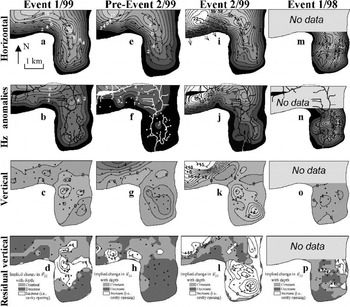
Fig. 7. Velocities in cm d−1 for event 1/99 (days 184.60–189.04, 1999), pre-event 2/99 (days193.92–196.60, 1999), event 2/99 (days 196.60–198.88, 1999) and event 1/98 (days 182.70–184.70, 1998), respectively:(a, e, i, m) horizontal; (b, f, j, n) horizontal anomalies (i.e. difference from winter 1999/2000; black lines mark reconstructed subglacial drainage pathways); (c, g, k, o) vertical; (d, h, l, p) residual vertical. Cavity opening is only likely where the assumption that wc = 0 requires
![]() to increase with depth relative to
to increase with depth relative to
![]() .
.
The relative increases in horizontal velocity during event 1/99 were spatially non-uniform: the mean velocity of stakes in the lower terminus increased by 110% relative to winter levels, while that of stakes in the upper terminus increased by 75% (Fig. 5b and c). Compared to winter, the central region of highest velocities broadened and there was a consequent narrowing of the marginal shear zones, particularly over the lower terminus and close to the snout (Figs 4a and 7a and b). The largest absolute velocity anomalies of up to 6 cm d−1 occurred over the upper terminus close to where winter velocities were highest, and close to the predicted subglacial drainage pathway there (Fig. 7b). Over the centre of the lower terminus, horizontal velocities were an almost constant 3 cm d−1 above winter levels (Fig. 7b), and there was a marked rotation of the surface velocity vectors (relative to the winter vectors) towards the west (Fig. 7a; cf. Fig. 4a). The rotation of the velocity vectors increased towards the glacier snout, where it reached >45° at some stakes.
There was little change in vertical velocity from winter levels, with most vertical velocities close to 0 cm d−1 (Figs 6 and 7c). Residual vertical velocity was also generally low, with only a limited area over the lower terminus where cavity opening is suggested by the apparent need for
![]() to increase with depth relative to
to increase with depth relative to
![]() (Fig. 7d).
(Fig. 7d).
Event 1/99 occurred at the end of the first week of intense summer melting (Fig. 8a). As indicated by the albedo and UDG records from the lower weather station, surface melting had been occurring for approximately 1 month prior to event 1/99 (Fig. 8b and c), although much of this melt may have refrozen in the cold snowpack. By the start of the event, the albedo had fallen to 40% (Fig. 8b), which defines the approximate boundary between a snow- and ice-covered surface (Reference PatersonPaterson, 1994, p. 59). The surface lowering rate was continuously positive during the event (Fig. 8d). The ice-marginal lake drained rapidly during event 1/99 (Fig. 9) (although it is not known when this drainage event started), and the first major discharges from the snout were observed during the overnight period between days 185 and 186. The largest geophone activity of the summer was recorded at the middle and lower geophones on day 186 (Fig. 8f and g). A further three smaller periods of activity were recorded at each of these geophones before the end of event 1/99, while no unusual counts were recorded at the upper geophone during this time (Fig. 8e).
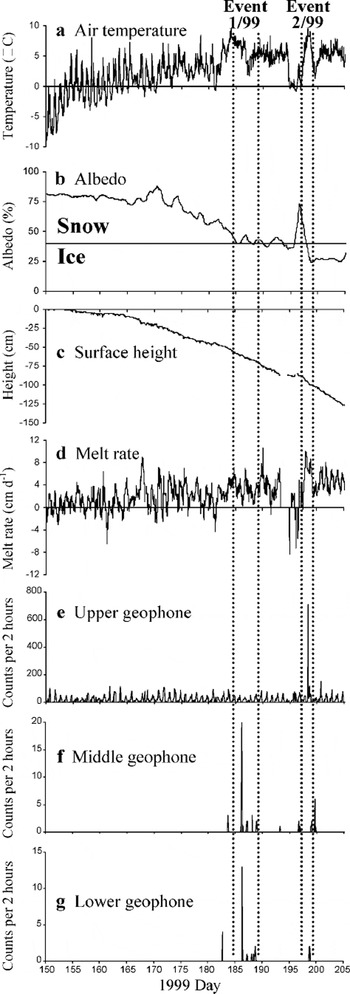
Fig. 8. (a–d) Summer 1999 lower-weather-station records: (a) air temperature; (b) albedo; (c) surface height measured from the start of the melt season; and (d) surface melt rate. Positive values indicate ablation, negative values indicate accumulation. (e–g) Summer 1999 geophone records: (e) upper geophone; (f) middle geophone; and (g) lower geophone. Note that only the relative magnitude of events is comparable between geophones, not the actual number of counts.
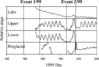
Fig. 9. Water-pressure records for summer 1999 (see Fig. 2 for sensor locations). The measurements are standardized between the highest and lowest values from each sensor over the period of interest.The proglacial sensor is repositioned during breaks.
3.2.2. Event 2/99: days 196.60–198.88
Event 2/99 saw large horizontal velocity increases at most stakes relative to both the preceding measurement period (days 193.92–196.60) and winter levels (Figs 4a, 5 and 7e, f, i and j). The horizontal velocity increases were highly spatially variable, as the increase in velocity of the stakes was much higher over the upper than over the lower terminus (Fig. 5b and c). On a local scale, the horizontal velocity increases over the lower terminus were focused on the eastern side, with velocities only a little above winter levels on the western side (Fig. 7j). Over the upper terminus, the largest velocity increases of the year occurred on the western side, with velocity anomalies up to 18 cm d−1, or ∼400%, above winter levels (Fig. 7j). These anomalies were localized above the predicted areas of subglacial water flow, and decreased rapidly towards the glacier margins. In addition, there was a strong rotation in horizontal velocity vectors towards the glacier margin in this area compared to both the winter and preceding measurement periods (Figs 4a and 7e and i). The rotation was greatest for stakes closest to the glacier edge which, in this region, consists of unsupported ice walls tens of metres high.
There were rapid and dramatic changes in vertical velocity during and prior to event 2/99, particularly over the upper terminus (Fig. 6). There was strong vertical uplift at most stakes during the event, compared to significant vertical lowering in the preceding measurement period (Figs 6 and 7g and k). For the lower-terminus stakes, vertical velocities averaged −1.4 cm d−1 in the preceding period and +1.0 cm d−1 during event 2/99 (Fig. 6b). For the upper-terminus stakes, mean vertical velocities were −1.1 cm d−1 in the preceding period and +3.5 cm d−1 during the event (Fig. 6c). As with horizontal velocity, these patterns are highly spatially variable, with the largest changes occurring over the western part of the upper terminus (Fig. 7g and k). At several stakes in this region, the change in rate of vertical velocity relative to the preceding period was >10 cm d−1.
Cavity opening would have been possible over only a limited area in the period prior to event 2/99 (Fig. 7h), but could have occurred over the entire lower terminus and the western part of the upper terminus during the event (Fig. 7l). In particular, the residual vertical velocity of >15 cm d−1 along the axis of predicted subglacial drainage over the western upper terminus is much higher than can be explained by changes in vertical strain rate with depth, and makes it likely that cavity opening occurred in this area.
During the 2 days prior to event 2/99, a storm system reduced air temperatures to below freezing and produced new snowfall (Fig. 8a). The albedo sensor records the increase in albedo due to the new snowfall (Fig. 8b), and the UDG records net accumulation during this period (Fig. 8c and d). Temperatures increased rapidly on day 197, and stayed well above freezing for the remainder of the event (Fig. 8a). Surface melting resumed as the weather warmed, and the highest sustained surface lowering rates of the summer occurred throughout event 2/99 (Fig. 8d).
All the water-level sensors showed a clear response to these weather changes (Fig. 9). Water levels were low at all locations during the cool period prior to event 2/99, and diurnal variability disappeared due to the reduction in meltwater supply. As air temperature and surface melt increased at the onset of event 2/99, water levels rose. Surface lowering rates peaked on day 198.1, water levels in the ice-marginal lake and supraglacial streams peaked between days 198.7 and 198.8, while the water level in the proglacial stream peaked on day 199.1 (Figs 8d and 9). The upper geophone recorded the largest number of events of the summer on day198 during event 2/99 (Fig. 8e). Smaller numbers of events, with counts well below those during event 1/99, were also recorded at the middle and lower geophones (Fig. 8f and g).
3.3. 1998 short-term velocity event
3.3.1. Event 1/98: days 180.71–184.71
Only one clear event was recorded in summer 1998 (Fig. 10). This event covers two measurement periods from days 180.71–182.71 and 182.71–184.71, with the largest and most significant horizontal velocity increases during the second half of the event (Fig. 10a). Consequently, only the velocity patterns from this second period are plotted (Fig. 7m–p).
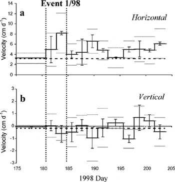
Fig. 10. Summer 1998 horizontal (a) and vertical (b) mean velocity (solid black line), winter 1999/2000 mean velocity (dashed line), errors in velocity (vertical bars), and standard deviation in velocity (grey lines). Six more stakes were added to the original network of 15 from day 185 onwards.
The mean horizontal velocity for the 15 stakes present during event 1/98 was 5.0 cm d−1 during the first half of the event, and 8.2 cm d−1 during the second half (Fig. 10a). This compares to a mean winter velocity for these stakes of 3.3 cm d−1. The high standard deviation in horizontal velocity (3.6 cm d−1) during event 1/98 implies either that the increases were not spatially uniform, or that there is large spatial variability in measurement errors (Fig. 10a). The highest velocity increases (up to 14 cm d−1) occurred over the eastern part of the lower terminus (Fig. 7n). This area of high horizontal velocities is defined by at least four stakes, and the velocity increases are well above error estimates. As in event 1/99, there was a rotation in the velocity vectors towards the west compared to winter patterns, and this was greatest close to the glacier snout (Figs 4a and 7m).
Vertical velocities varied little and were close to winter values during event 1/98 (Figs 7o and 10b). Of the 15 stakes measured during the event, most had vertical velocities of 0 to −1 cm d−1. The residual vertical velocity averaged ∼0 cm d−1, and there were few areas where cavity opening may have occurred (Fig. 7p).
As with event 1/99, event 1/98 occurred during a period of rapid melting approximately 30 days after the start of the melt season. Air temperatures were higher than at any previous time in 1998, and remained well above freezing throughout (Fig. 11a). Approximately 95 cm of surface lowering occurred in the month prior to event 1/98 as the surface snow cover melted (Fig. 11c), and melt rates reached their highest sustained levels of the summer during the event (Fig. 11d).
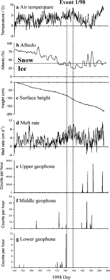
Fig. 11. Same as Figure 8, but for summer 1998.
Event 1/98 coincided with the initiation of subglacial outflow from the terminus. This occurred primarily via an artesian fountain on the lower eastern terminus on day 180 (Fig. 3), which reached its peak height during days 182–184, before declining around day 186. The fountain reached heights of 5 m, and brought large volumes of relatively turbid, high-EC water to the glacier surface through an ice thickness of ∼70 m (measured by radio-echo sounding; Reference Copland and SharpCopland and Sharp, 2001). This suggests a subglacial origin for the water, and indicates that basal water pressures were ∼120% of ice overburden pressure over at least part of the lower terminus. Longitudinal fracturing of the ice surface was observed around the artesian fountain, with most fracturing occurring when the fountain first emerged. This fracturing was recorded by a small number of events at the middle geophone around day 180.25, and by a large number of events at the lower geophone around day 180.46 (Fig. 11f and g). No significant activity was recorded at the upper geophone at this time (Fig. 11e).
4. Discussion
From these measurements, it is evident that short-term velocity events are associated with periods of rapidly increasing meltwater inputs to the subglacial drainage system. Similar relationships have also been observed during short-term high-velocity events on temperate and predominantly warm polythermal glaciers (e.g. Reference Iken and BindschadlerIken and Bindschadler, 1986; Reference JanssonJansson, 1995; Reference Mair, Nienow, Willis and SharpMair and others, 2001) and on the Greenland ice sheet (Reference Zwally, Abdalati, Herring, Larson, Saba and SteffenZwally and others, 2002). At John Evans Glacier, the first velocity event of the melt season typically occurs about 1 month after the onset of melt, when the connection between the supraglacial and subglacial drainage systems is first established and subglacial outflow begins (events 1/98 and 1/99). A subsequent event occurred later in the melt season, when melt resumed after a prolonged cold spell (event 2/99).
4.1. Early-season events
Rising water inputs during early-season events are due to a combination of warm weather, high rates of surface melt, and the drainage of supraglacial and ice-marginal lakes within and at the upstream ends of the supraglacial channel systems (Figs 8a and d, 9 and 11a and d). Outflow of subglacially routed waters at the glacier terminus typically begins within 24 hours of surface waters starting to drain into the glacier via the crevasse field at the top of the terminus. This is probably because the new water input pressurizes the existing subglacial reservoir beneath the lower terminus, driving outlet development at the snout. Evidence for pressures above ice overburden levels is provided by the formation of the artesian fountain, while the high EC of the first waters to be released is indicative of long subglacial residence times. Fracturing associated with outlet development likely contributes to the high counts recorded at the lower geophone during events 1/99 and 1/98 (Figs 8g and 11g).
High horizontal velocities at this time are presumably linked to high basal water pressures (and possibly increasing subglacial water storage), which reduce basal friction and enhance basal velocity. The PCA scores for the factor 1 stakes reached their highest values during event 1/99 (Fig. 5d), as the largest horizontal velocity changes of the year occurred over the lower terminus (Fig. 7a and b). This suggests that the frozen snout provided the greatest hydraulic resistance to outflow of subglacial waters at this stage of the melt season. The increasingly large westward rotation of the horizontal velocity towards the snout compared to winter patterns (Figs 4a and 7a and m) suggests that the frozen margin also impeded the flow of the warm-based ice upstream. This resulted in compression and left-lateral shearing in the region of the warm–cold transition at the glacier bed. Within the warm-based region, there was a close association between the area of highest horizontal velocity anomalies during event 1/98 and the locations of both the predicted subglacial water flow and the artesian fountain (Fig. 7n; see Fig. 2 for location of artesian fountain). This suggests that the hydrological forcing responsible for enhanced basal velocity may have been strongest in the vicinity of major subglacial drainage axes.
4.2. Mid-season event
Event 2/99 occurred after a prolonged cold period during which there was snowfall, surface melt ceased (Figs 8a, b and d), and water levels dropped in all monitored streams (Fig. 9). It is likely that subglacial water pressures dropped at this time as meltwater inputs to the glacier interior decreased. Depending on the subglacial drainage configuration, this would have allowed closure of basal cavities or subglacial channels by ice and/or basal sediment deformation, and/or compaction of the glacier bed due to a reduction in the porosity of basal sediment. All of these processes would result in net surface lowering, as was observed in areas close to the subglacial drainage pathways in the period prior to event 2/ 99 (Fig. 7g). The highest rates of lowering during this period occurred in the northwest part of the upper terminus where the ice thicknesses are greatest (200–250 m) (Reference Copland and SharpCopland and Sharp, 2001). The inferred reduction in basal water pressure would have also increased basal drag, accounting for the relatively low horizontal velocities at this time (Fig. 7f).
Melt resumed as the weather warmed at the start of event 2/99 (Fig. 8a and d), with a rapid rise in water levels at all monitoring locations (Fig. 9). At this time, water levels in the supraglacial streams reached their highest levels since event 1/ 99, indicating that a large meltwater pulse entered the subglacial drainage system via the crevasse field at the top of the terminus. Event 2/99 was characterized by extremely high horizontal and vertical velocities in the area immediately above the predicted location of the subglacial drainage axis beneath the western part of the upper terminus (Fig. 7i–k). The large number of counts registered at the upper geophone at this time (Fig. 8e), together with the high PCA factor 2 scores (Fig. 5d), supports the fact that event 2/99 was centred over the upper terminus.
The very pronounced velocity response in the northwest region of the terminus at this time suggests that basal water pressures may have risen to very high levels in this area when meltwaters were reintroduced to the bed following the cold period. The inferred rates of cavity opening in this area suggest that extensive ice–bed decoupling may have resulted (Fig. 7l). This behaviour was likely a response to the contraction of drainage channels beneath the thick ice in this area during the preceding cold period, which impeded meltwater drainage across this section of the glacier bed. The strong southward rotation of the velocity vectors in this area (Fig. 7i; cf. Fig. 7e) implies that normal glacier flow towards the east-northeast was impeded at this time. This can be explained by a downflow increase in basal drag arising from a downstream collapse or reduction in size of the subglacial drainage channels.
Over the lower terminus, horizontal and vertical velocities during event 2/99 were lower than in the western part of the upper terminus, but they reached peak values above the eastern drainage axis (Fig. 7j and k). Inferred rates of basal cavity opening were also highest in this area, although cavity opening appears to have occurred across the whole lower terminus region (Fig. 7l). This is somewhat problematic given the argument above that the large velocity response in the upper terminus region is attributable to closure of major drainage channels downstream from this region. Such closure, if complete, would presumably have prevented transfer of subglacial water to the lower terminus. There are two possible resolutions to this: (i) incomplete closure allowed some basal water flow to the lower terminus, but still caused backing up and high water pressure below the upper terminus; (ii) the reopening of channels led to a delayed water input to the lower terminus, causing the velocity event there to lag the one in the upper terminus. Unfortunately, the resolution of the velocity measurements is too coarse to show whether the velocity events in the upper and lower terminus regions were exactly synchronous.
4.3. Comparisons between events
A comparison of the horizontal and vertical velocities associated with events 1/98 and 1/99 reveals some interesting differences. In 1998, the largest horizontal velocity anomalies were associated with the eastern subglacial drainage axis (Fig. 7n), while in 1999 they were less pronounced and more widely distributed (Fig.7b).Vertical velocities during events 1/98 and 1/99 were generally low (Fig. 7c and o), with cavity opening restricted to a small area on the western side of the lower terminus during event 1/99 (Fig. 7d and p). The smaller magnitude of the event 1/99 horizontal velocity anomalies suggests that basal water pressures did not rise as high as in event 1/98, which is consistent with the observation that no artesian fountain formed on the glacier surface in 1999. One possible explanation is that large subglacial channels formed during the exceptionally warm summer of 1998 did not close completely during winter 1998/99, and that they allowed more efficient drainage of the initial water inputs to the glacier bed in early summer 1999. This could explain the limited area of cavity opening during event 1/99, although the generally small vertical velocity response during the early-season events makes it likely that subglacial drainage was mainly distributed at this time.
The form of the horizontal velocity anomalies over the lower terminus during event 2/99 provides some evidence for the reorganization of subglacial drainage (Fig. 7j). The anomalies suggest that the hydrological forcing for this event was associated with the eastern drainage axis, and thus different from the more widespread forcing that seems to have been associated with event 1/99 (Fig. 7b). As discussed above, event 1/98 also appears to have been forced from the eastern drainage axis (Fig. 7n), although there are significant differences in the ice velocity responses associated with the two events in the lower terminus region. Horizontal velocity anomalies were higher and more widespread in event 1/98 (Fig. 7j and n), whereas cavity opening was more widespread during event 2/99, with a peak along the eastern drainage axis (Fig. 7l and p). These differences may reflect differences in the amounts of water entering the glacier and in the character of the subglacial drainage system between the two events. Event 1/98 was associated with the first input of surface water to the glacier bed during summer 1998, and occurred when much of the glacier upstream from the crevasse field was still snow-covered. Event 2/99, by contrast, occurred when glacier ice was exposed over much of this area. Given that air temperatures reached similar high values during both events (Figs 8a and 11a), melt production in the area draining into the crevasse field was likely higher during event 2/99.
From these observations it appears that there is both interannual and intra-annual variability in the pathway by which meltwater which penetrates to the glacier bed drains to the glacier terminus. It appears that water draining subglacially from the upper terminus can, at different times, connect to either or both of the eastern and western drainage axes beneath the lower terminus. The likely location of the connection between the two axes is apparent from the form of the contours in Figure 7j.
5. Conclusions
Measurements over 2 years demonstrate that, in summer, surface meltwater penetrates significant thicknesses (>200 m) of cold ice to reach the glacier bed and affect the horizontal and vertical surface velocities of John Evans Glacier. Horizontal surface velocities are higher in summer than in winter across the entire glacier terminus. High-velocity events lasting 2–4 days occur during periods of rapidly increasing meltwater input to the glacier interior. Horizontal velocities during these events reach up to 400% of winter velocities.
Early-summer velocity events are linked to the initiation of supraglacial water inputs to the glacier bed. These initial inputs include the drainage of significant volumes of water previously stored in supraglacial and ice-marginal lakes. A mid-summer event occurred during a period when melt rates increased rapidly following cold weather and new snowfall. All events are probably a result of high, and rapidly rising, subglacial water pressures and/or water storage.The horizontal and vertical velocity anomalies that result differ significantly between events. This is probably a result of seasonal and interannual changes in the routing of meltwater across the bed and in the nature of the subglacial drainage system. Early-season events are initiated within a predominantly distributed subglacial drainage system, while the mid-summer event appears to have been initiated within a channelized subglacial drainage system that had undergone significant closure immediately prior to the event during a cold period with limited meltwater drainage to the bed.
The results of this study indicate a strong coupling between the surface velocity of a predominantly cold polythermal glacier, the magnitude and distribution of surface water inputs to the englacial/subglacial drainage system, and the distribution, formation and seasonal evolution of subglacial drainage pathways. The surface velocity of the glacier is extremely sensitive to rapid increases in the delivery of surface waters to the glacier bed. This behaviour is qualitatively comparable to that seen on both temperate and warm polythermal glaciers (Reference Iken and BindschadlerIken and Bindschadler, 1986; Reference JanssonJansson, 1995; Reference Kavanaugh and ClarkeKavanaugh and Clarke, 2001; Reference Mair, Nienow, Willis and SharpMair and others, 2001) and on the Greenland ice sheet (Reference Zwally, Abdalati, Herring, Larson, Saba and SteffenZwally and others, 2002). A number of characteristics that may be typical of predominantly cold polythermal glaciers influence the details of the behaviour observed. These include the thermal barrier to the flow of ice and basal water at the snout and margins of the glacier, the sudden onset of subglacial drainage in the early summer, and the importance of water inputs from ice-marginal and supraglacial lakes.
Acknowledgements
Funding was provided by the Natural Sciences and Engineering Research Council of Canada, the U.K. Natural Environment Research Council ARCICE programme, the Geological Society of America, the University of Alberta Izaak Walton Killam Memorial Scholarship, and the Canadian Circumpolar Institute of the University of Alberta. Logistic support was provided by the Polar Continental Shelf Project, Natural Resources Canada (contribution No. 023-01). We thank the Nunavut Research Institute and the communities of Grise Fiord and Resolute Bay for permission to work atJohn Evans Glacier, andW. Davis, D. Glowacki, A. Arendt, T. Wohlleben, R. Bingham and J. Davis for help in the field. C. S. Hvidberg (Scientific Editor), J. Kavanaugh and P. Jansson provided useful comments on the manuscript.


