


Introduction
Ice thickness is a crucial initial condition for projecting future glacier change, ice mass remaining and runoff in glacierised regions (Pieczonka and others, Reference Pieczonka, Bolch, Kröhnert, Peters and Liu2018; Helfricht and others, Reference Helfricht, Huss, Fischer and Otto2019). However, it is difficult to directly measure the thickness of all glaciers at a regional or national scale (Langhammer and others, Reference Langhammer, Grab, Bauder and Maurer2019; Pritchard and others, Reference Pritchard2020; Werder and others, Reference Werder, Huss, Paul, Dehecq and Farinotti2020). The Glacier Thickness Database (GlaThiDa) collects measured ice thickness data worldwide (Welty and others, Reference Welty2020). The latest release GlaThiDa v3 includes ice thickness records for more than 3000 glaciers around the world (Welty and others, Reference Welty2020), yet this is still a small number compared with the 215 000 glaciers worldwide. For the remaining glaciers, ice volume was once estimated using scaling relationships between glacier volume (or mean ice thickness) and glacier geometric metrics (usually area or length; Bahr and others, Reference Bahr, Meier and Peckham1997; Grinsted, Reference Grinsted2013; Guo and others, Reference Guo2015). Since such scaling relationships cannot provide spatial ice distribution, a series of ice thickness inversion models have been developed (Farinotti and others, Reference Farinotti, Huss, Bauder, Funk and Truffer2009a; Huss and Farinotti, Reference Huss and Farinotti2012; Linsbauer and others, Reference Linsbauer, Paul and Haeberli2012; Frey and others, Reference Frey2014; Gantayat and others, Reference Gantayat, Kulkarni and Srinivasan2014; Fürst and others, Reference Fürst2017). Recently, modelled ice thickness (Farinotti and others, Reference Farinotti2019) has been widely used as a boundary condition for large-scale models which study future glacier mass loss under climate change (Huss and Hock, Reference Huss and Hock2018; Zekollari and others, Reference Zekollari, Huss and Farinotti2019; Khadka and others, Reference Khadka, Kayastha and Kayastha2020; Rounce and others, Reference Rounce, Hock and Shean2020).
Glaciers in the Tian Shan range (hereafter the Tian Shan) are one of the most important fresh water contributors in Central Asia, providing water to a local population of more than 20 million (Farinotti and others, Reference Farinotti2015; Luo and others, Reference Luo2018; Armstrong and others, Reference Armstrong2019; Hoelzle and others, Reference Hoelzle, Xenarios, Schmidt-Vogt, Qadir, Janusz-Pawletta and Abdullaev2019). In some headwater catchments, the glacier contribution to the total runoff can be nearly 70% in summer (Sorg and others, Reference Sorg, Bolch, Stoffel, Solomina and Beniston2012; Saks and others, Reference Saks2022). Consistent with the increasing temperatures, most glaciers in the Tian Shan have displayed a noticeable retreat since the 1960s (Chen and others, Reference Chen, Li, Deng, Fang and Li2016). In the short term, shrinking glaciers supply more fresh water and protect against water shortages. For example, glacier mass loss could provide over 50% of the runoff inputs in some Aral sub-basins in a drought year (Pritchard, Reference Pritchard2019). However, by the end of the 21st century the Tian Shan glacier runoff could decrease by ~20–50% (Huss and Hock, Reference Huss and Hock2018; Rounce and others, Reference Rounce, Hock and Shean2020), which could threaten local water availability and food security in the future (Immerzeel and others, Reference Immerzeel, van Beek and Bierkens2010; Viviroli and others, Reference Viviroli, Kummu, Meybeck, Kallio and Wada2020).
Despite the importance of glaciers in the Tian Shan, few studies have specifically investigated ice thickness of all the glaciers in this region. Previous studies have either considered this region in the context of glaciers worldwide (Huss and Farinotti, Reference Huss and Farinotti2012; Farinotti and others, Reference Farinotti2019), or investigated several individual glaciers (Li and others, Reference Li, Ng, Li, Qin and Cheng2012; Pieczonka and others, Reference Pieczonka, Bolch, Kröhnert, Peters and Liu2018; Van Tricht and others, Reference Van Tricht2021). Due to the limited availability of measured glacier thickness and because global studies have different research aims, considerable uncertainty remains at the regional scale (Helfricht and others, Reference Helfricht, Huss, Fischer and Otto2019; Pelto and others, Reference Pelto, Maussion, Menounos, Radić and Zeuner2020). Besides, there are errors and discrepancies in the Randolph Glacier Inventory version 6 (RGI v6) due to its provenance (Pfeffer and others, Reference Pfeffer2014; RGI Consortium, 2017; Herreid and Pellicciotti, Reference Herreid and Pellicciotti2020), yet the effects of these errors on subregional ice volumes and projections are unknown. Fortunately, the updated Glacier Area Mapping for Discharge from the Asian Mountains (GAMDAM v2, Sakai, Reference Sakai2019) provides an independent, alternative inventory data source which can help to assess the importance of these uncertainties.
Therefore, we aim to provide new estimates of the distributed ice thickness in the Tian Shan range, complementing previous global research (Farinotti and others, Reference Farinotti2019). We also discuss the potential influence of the inventories and digital elevation models (DEMs) on the estimation and projection of glacier mass in the remaining decades of this century. Based on the Open Global Glacier Model (OGGM) developed by Maussion and others (Reference Maussion2019) and methods developed by Li and others (Reference Li, Ng, Li, Qin and Cheng2012) and Linsbauer and others (Reference Linsbauer, Paul and Haeberli2012), we built an inverse model which determines ice thickness by its relationship to basal shear stress (hereafter BS model). The mass conservation inverse model (hereafter MC model) integrated in the OGGM is also used and compared to the BS model. The inverse models are calibrated and validated against the observed ice thickness data in the GlaThiDa v3. The regional ice thickness is then estimated using the calibrated inverse models. Furthermore, we project the remaining glacier mass from 2018 to 2100 utilising the glacier evolution model in the OGGM based on both the RGI v6 and GAMDAM v2 to test the influence of ice volume and glacier inventory on projections of future glacier change.
Study area
The Tian Shan is located in Central Asia, across Uzbekistan, Kazakhstan, Kyrgyzstan and China (Fig. 1). There are four main hydrological regions (Aralo-Caspian, Balkhash, Issik Kul and Tarim) in the Tian Shan, which are all endorheic drainages (Aizen and others, Reference Aizen, Aizen, Melack and Dozier1997). To the south, water from the Tian Shan mountains flows into the Tarim Basin, supporting the fragile ecosystem on the northern edge of the Taklimakan Desert (Pieczonka and Bolch, Reference Pieczonka and Bolch2015). To the west, the water irrigates large tracts of farmland in Kyrgyzstan, Kazakhstan and Uzbekistan (Chen and others, Reference Chen, Li, Fang and Li2018). Peak Tomur, 7439 m a.s.l, is the highest peak and is located in the central zone of the Tian Shan region. Seven glaciers with an area of more than 100 km2 in the Tian Shan are all distributed around it. For both the RGI v6 and GAMDAM v2, the glacierised area is ~1.2 × 10⁴ km2, covering ~2.7% of the land surface (RGI Consortium, 2017; Sakai, Reference Sakai2019). Glacier properties in the Tian Shan are varied and complex (Brun and others, Reference Brun2019; Barandun and others, Reference Barandun2021). While most glaciers experienced a retreat during the last decades (Farinotti and others, Reference Farinotti2015), there have been reports of advancing or surging glaciers (Li and others, Reference Li2017; Mukherjee and others, Reference Mukherjee2017; Zhou and others, Reference Zhou2021).

Fig. 1. Map of glaciers, international borders and topography in the Tian Shan, Central Asia. The glacier data are from the GAMDAM v2 (Sakai, Reference Sakai2019). Country borders are shown here because of the various data sources in the RGI v6 which follow country borders. The eight reference glaciers are Sary Tor (ST), Tsentralniy Tuyuksu (TYK), Heigou No. 8 (HG), Haxilegen No. 51 (HXLG), Sigonghe No. 4 (SGH), Urumqi No.1 West Branch (UMW), Urumqi No.1 East Branch (UME) and Qingbingtan No. 72 (QBT).
Data
Measured ice thickness
The GlaThiDa is a continuously updated collection of ice thickness measurements worldwide (Welty and others, Reference Welty2020). There are eight Tian Shan glaciers represented in the GlaThiDa v3 (Fig. 2), together accounting for 14 925 points with ice thickness measured by ground-penetrating radar (GPR). This represents a great advance over the GlaThiDa v2, which only included measurements from four glaciers in the Tian Shan. The eight glaciers therefore serve as reference glaciers to calibrate model parameters, validate model performance and investigate model sensitivity and uncertainty. Among the eight reference glaciers, HG (Heigou No. 8 glacier) has both the maximum point thickness (178 m) and average thickness (114.2 m). The minimum average glacier ice thickness is observed in QBT (Qingbingtan No. 72 glacier, 39.1 m), despite it being the largest reference glacier apart from HG (Table 1). We gridded the point thickness data to the pixel of the model output thickness raster if there were two or more points on one pixel (see Methods section for details of the raster resolution). Otherwise, the point thickness data represent the measured thickness of the pixel. The average of all gridded observations of ice thickness across our eight reference glaciers is 65.8 m (Table 1). In the GlaThiDa v3, the ice thickness of UME (Urumqi No. 1 Glacier East Branch) and UMW (Urumqi No. 1 Glacier West Branch) was reported twice in 2006 and 2014. In this study, we have used the 2014 data. All of the measured ice thickness data used in this study were surveyed between 2008 and 2014.

Fig. 2. Glacier outlines and measured ice thickness for the reference glaciers. The ice thickness has been derived from the GlaThiDa v3.
Table 1. Glacier ID in the GlaThiDa v3 (GlaThiDa ID), latitude (Lat.), longitude (Lon.), glacier area (Area) in 2000 and 2013, ice thickness survey year (Survey year), number of observations (Num.), mean ice thickness for observation points $( \bar{h}_{{\rm obs}})$ and mean ice thickness for pixels $( \bar{h}_{{\rm pix}})$

Newly added glaciers in the GlaThiDa v3 are shown in bold.
Topography
In order to investigate the influence of different topography at different timestamps on the ice thickness inversion result, two DEMs were used: the Shuttle Radar Topography Mission (SRTM) DEM Version 4 (Jarvis and others, Reference Jarvis, Reuter, Nelson and Guevara2008) and the Copernicus DEM GLO-90 (https://spacedata.copernicus.eu/). The SRTM launched on 11 February 2000. Interferometry was used for terrain by employing a single-pass dual-antenna synthetic aperture radar (SAR) over the following 11 days. The SRTM acquired images at both X- and C-band. The C-band SRTM DEM with global coverage (3 arcsec, ~90 m resolution) is widely used (Reuter and others, Reference Reuter, Nelson and Jarvis2007; Jarvis and others, Reference Jarvis, Reuter, Nelson and Guevara2008). The vertical and horizontal accuracy are 16 and 20 m (both with 90% confidence level) (Rabus and others, Reference Rabus, Eineder, Roth and Bamler2003). The SRTM DEM version 4 is the improved version of the original SRTM DEM by filling ‘no data’ holes. In this study, the SRTM DEM version 4 (hereafter SRTM) was used for the topography in 2000. The Copernicus DEM is a global DEM and reprocessed from WorldDEMTM products by resampling, filling holes, replacing abnormal values, etc. The source data for WorldDEMTM were acquired during the 2011–2015 TanDEM-X mission. The Copernicus DEM is also derived from SAR images but at X-band. There are currently three Copernicus DEM products, EEA-10, GLO-30 and GLO-90, with resolutions of 10, 30 and 90 m, respectively. The vertical and horizontal accuracy of the Copernicus DEM are 4 and 6 m (both with 90% confidence level, https://spacedata.copernicus.eu/). Here, we have used the Copernicus DEM GOL-90 (hereafter COPDEM) to reflect the topography around 2013.
Glacier inventories
To match the acquisition time of the reference glacier outlines to the DEM, we used 14 Landsat scenes as close as possible to 2000 and 2013 to draw the outlines of these eight reference glaciers (Fig. 2). Since we were not able to find suitable Landsat images from 1998 to 2002, QBT glacier was not included in the glacier outlines (2000). Glacier outlines (2013) were used to optimise the model parameters combined with the COPDEM and measured ice thickness data. Also, the inverse ice thickness in glacier outlines (2000) and glacier outlines (2013) was compared to test the response of our inverse models to glacier area change.
To estimate ice thickness on a regional scale, two glacier inventories (RGI v6 and GAMDAM v2) were used. The RGI v6 contains two main data sources for the Tian Shan range: the second Chinese Glacier Inventory (CGI v2) (Guo and others, Reference Guo2015) for glaciers in China and the GAMDAM v1 for glaciers in other countries. The reason the RGI v6 used the CGI v2 for glaciers in China is because the GAMDAM v1 underestimates glacier area in headwall regions (Pfeffer and others, Reference Pfeffer2014; RGI Consortium, 2017). While for glaciers in other countries, the GAMDAM v1 (RGI Consortium, 2017) is the only inventory available. Therefore, there are systematic differences between glaciers in China and in other countries, due to the different methodologies and data sources. The GAMDAM v1 is manually distributed based on Landsat images from 1999 to 2003 (Nuimura and others, Reference Nuimura2015). The CGI v2 is a semi-automated product based on Landsat images from 2006 to 2010 (Guo and others, Reference Guo2015).
To address the shortcomings of the GAMDAM v1, Sakai (Reference Sakai2019) released GAMDAM v2, which not only corrects the missing glacier area in the headwalls, but also includes more summer remote-sensing images to avoid inaccuracies caused by seasonal snow. In order to avoid the systematic error in the GAMDAM v2 caused by different operators, the author manually delineated the outline of each glacier.
In total, there are 19 304 glaciers with an area of 11 685.0 km2 in the GAMDAM v2 and 13 881 glaciers with an area of 11 826.7 km2 in the RGI v6 in the Tian Shan. The difference of glacier area between the two inventories is only ~1%. However, there are large regional differences: the RGI v6 glacier area is ~10% (664.2 km2) more than the GAMDAM v2 in China and ~10% (531.9 km2) less in other countries. Taking the glaciers near Peak Tomur as an example (Fig. 3), it is obvious that RGI v6 overestimates the area of Tomur Glacier (in China). On the other hand, for South Inylchek Glacier (in Kyrgyzstan), the GAMDAM v2 tends to cover more surface due to the added headwall regions. Figure 4 shows the date distribution of glacier outlines in both inventories. In RGI v6 (Fig. 4), there are two main periods (1998–2002 and 2006–2007) indicating that the data are from the GAMDAM v1 and CGI v2 specifically. The GAMDAM v2 has a longer but more continuous survey period (1994–2008) than the RGI v6, with ~70% of the glacier outlines dated between 1998 and 2002.

Fig. 3. Example of the difference in glacier outlines between the GAMDAM v2 and the RGI v6.

Fig. 4. Date of glacier outlines in the RGI v6 and GAMDAM v2 in the Tian Shan region. The ordinate shows the survey years. The numbers next to the bars show the glacier numbers in China as well as in other countries for that year.
Methods
Due to its open source and modular framework, we chose the OGGM as the platform for this study. The OGGM was developed by Maussion and others (Reference Maussion2019). Its functionality encompasses flowline extraction, ice thickness inversion and glacier evolution simulation. The OGGM provides various public geographical and meteorological data, such as DEMs, mass balance and gridded climate data, and allows users to work with their own data, such as glacier inventory and DEMs. It reprojects DEMs onto a local map centred around each glacier. The target resolution of the reprojected DEM and other gridded outputs is determined by the glacier area and cropped to the 10–200 m range (e.g. a glacier of size 8 km2 will have a resolution of ~50 m while large glaciers with area over 200 km2 will all have a resolution of 200 m; Maussion and others, Reference Maussion2019). The reprojected DEMs are smoothed with a Gaussian filter of size 250 m.
A temperature index melt model presented by Marzeion and others (Reference Marzeion, Jarosch and Hofer2012) is used to compute the mass balance M at an elevation z in OGGM:

where p f (default 2.5) is a factor used to correct the gridded precipitation to orographic precipitation, $P_i^{\rm S}$ and T i are the monthly solid precipitation and air temperature, μ* is the temperature sensitivity of the glacier, T M is the monthly mean air temperature above ice melt, and ε is a residual bias correction. As in Maussion and others (Reference Maussion2019), we used observed glaciological mass-balance data from the Fluctuations of Glaciers (FoG; WGMS, 2020) database to calibrate the mass-balance model. The downscaled Climatic Research Unit gridded Time Series version 4.03 (CRU TS4.03) dataset (see below) is used as the climate input of the mass-balance model. For more information about the procedure, see Marzeion and others (Reference Marzeion, Jarosch and Hofer2012) and Maussion and others (Reference Maussion2019). It must be noted here that the calibration procedure has only a slight influence on the estimated ice thickness (because of the steady-state assumption).
The CRU TS4.03 is a grid reanalysis climatic dataset with 0.5o × 0.5o spatial resolution and monthly time resolution (Harris and others, Reference Harris, Osborn, Jones and Lister2020). The dataset spans the years 1901–2018 and covers all of the continents excluding Antarctica. It was then downscaled to 10′ × 10′ resolution employing the CRU CL v2.0 dataset (New and others, Reference New, Lister, Hulme and Makin2002). During the projection procedure, the GCM climate data at each glacier location are bias-corrected using the previously downscaled CRU TS4.03 based on the delta method for the reference period 1981–2018, following the standard OGGM bias correction procedures (as in, e.g. Huss and Hock, Reference Huss and Hock2015).
Ice thickness inversion models
Our first ice thickness inversion module is a MC model currently used as default in the OGGM. It is built on the shallow-ice approximation, and somewhat similar to the Ice Thickness Estimation Method (ITEM) (Farinotti and others, Reference Farinotti, Huss, Bauder, Funk and Truffer2009a). The main difference between the two models is the approach chosen for the ‘apparent mass balance (AMB)’. The AMB (introduced by Farinotti and others, Reference Farinotti, Huss, Bauder, Funk and Truffer2009a) is the difference between the climatic mass balance and total local ice deformation at a given point. For glaciers in steady state, the thinning rate is negligible and AMB is equal to the climatic mass balance. Since the AMB is unknown, the ITEM uses an empirical relationship between equilibrium line altitude and vertical mass-balance gradient to determine the AMB (Farinotti and others, Reference Farinotti, Huss, Bauder, Funk and Truffer2009a), while the OGGM assumes that the glaciers are in steady state and uses calibrated climatic mass-balance (Eqn (1)) estimates instead.
In addition to the MC model, we also built a BS model based on the OGGM flowline and interpolation program. In this approach, the ice thickness (h) along the central flow lines can be calculated with Eqn (2) (Li and others, Reference Li, Ng, Li, Qin and Cheng2012).

where $\rho = 900\,{\rm kg\ }{\rm m}^{{-}3}$ is the ice density, $g = 9.81\,{\rm m\ }{\rm s}^{{-}2}$
 is the gravity acceleration, f = 0.8 (Linsbauer and others, Reference Linsbauer, Paul and Haeberli2012; Frey and others, Reference Frey2014; Van Tricht and others, Reference Van Tricht2021) is the shape factor, τ (in Pa) is the basal shear stress and α is the surface slope along the central flowlines computed with the topography data. The flowline slope is smoothed with a 1D Gaussian filter of kernel size 1.
Basal shear stress τ normally is determined by an elevation-range (Δh, in km) empirical relationship proposed by Maisch and Haeberli (Reference Maisch and Haeberli1982):

Once the thickness along the flow lines is determined, the ice thickness can be distributed using an interpolation method implemented in the OGGM. First, ice thickness on each pixel is interpolated from the centreline locations within a 100 m altitude range using inverse distance weighting. Then, a first weight determined by the distance between the pixel and the glacier outline was used to ensure that ice thickness tends towards zero at the glacier outline. Following Farinotti and others (Reference Farinotti, Huss, Bauder, Funk and Truffer2009a, Reference Farinotti, Huss, Bauder and Funk2009b), a second weighting factor determined by the slope of the pixel was applied to take the influence of glacier surface slope into account. The relative strength of each of the two weighting factors was optimised during the OGGM contribution to Farinotti and others (Reference Farinotti2019) and computed so that the total glacier volume is preserved after interpolation.
Projection of glacier volume
To assess the influence of different glacier inventories on future glacier change, we also projected the ice volume from 2000 to 2100 based on the ice thickness from the MC and ice dynamics module of the OGGM. The module is driven by CRU TS4.03 climate data from 2000 to 2018. Geodetic mass-balance observations (Shean and others, Reference Shean2020) were used to eliminate the bias between the default OGGM simulated mass balance and geodetic mass balance at the regional scale by correcting the residual ε in Eqn (1). For projections, the model is forced using general circulation model (GCM) projections archived in the Coupled Model Intercomparison Project Phase 6 (CMIP6). A total of 15 GCMs (BCC-CSM2-MR, CAMS-CSM1-0, CESM2, CESM2-WACCM, CMCC-CM2-SR5, EC-Earth3, EC-Earth3-Veg, FGOALS-f3-L, GFDL-ESM4, INM-CM4-8, INM-CM5-0, MPI-ESM1-2-HR, MRI-ESM2-0, NorESM2-MM, TaiESM1) with four CMIP6 shared socioeconomic pathways (SSP1-2.6, SSP2-4.5, SSP3-7.0 and SSP5-8.0) were used to determine glacier change from 2018 to 2100. We did not take surging into account for this study and discuss potential implications in the Discussion section. Figure 5 shows the main workflow of our ice thickness inversion and mass projection procedure.

Fig. 5. Flowchart showing the workflow of ice thickness inversion and mass projection procedures.
Ice thickness model calibration and validation
In this study, the Glen ice creep parameter A in the MC model and the basal shear stress τ are the target parameters for improving model performance. The A parameter (default 2.4 × 10⁻²⁴s−1Pa−3) is the physical quantity that characterises ice temperature and hardness. A larger A reflects a warmer/softer ice, resulting in thinner ice. According to Maussion and others (Reference Maussion2019), the influence of A for the estimated ice thickness follows a logarithmic relationship. This relationship makes the estimated ice thickness more sensitive to a change in A towards smaller values than a change towards larger ones. In the BS model, τ is linearly related to the estimated ice thickness (Eqn (2)). While these parameters have a physical meaning, in the following they are also used as calibration and bias correction parameters (e.g. overestimation of solid precipitation in the OGGM can be compensated by a larger A) and should therefore not be overinterpreted.
Here, we keep the tuning parameters constant for all glaciers in the Tian Shan, and the eight reference glaciers are considered together. We adjusted the target parameters by multiplying them to a calibration parameter (p). To determine the optimal p (p opt), a cross-validation process following Pelto and others (Reference Pelto, Maussion, Menounos, Radić and Zeuner2020) was used:
(i) Divide the measured ice thickness points of each reference glacier into a training group (80%) and a test group (20%) randomly.
(ii) Divide the training group points obtained in step (i) into a calibration group and a validation group (50% each) randomly.
(iii) Run the thickness inverse model and calculate the mean absolute error (MAE) by comparing the simulated thickness with measured thickness for all the reference glaciers in the calibration group.
(iv) Adjust p until the minimum MAE is produced, then take the p value as the alternative.
(v) Run the thickness inversion model again with the alternative p value and calculate the MAE between the simulated thickness and the measured thickness in the validation group.
(vi) Repeat steps (ii–v) 50 times and set the alternative p value with the minimum MAE in the validation group as the p opt to simulate the thickness in the future.
(vii) Run the thickness inverse model with p opt and calculate the MAE between simulation thickness and the test group measured thickness to estimate the simulation thickness error (σ T).
During the cross-validation process, we used the manual glacier outlines (2013) and the COPDEM to minimise the possible thickness uncertainty caused by survey time gap. Besides simulating ice thickness, the optimised A mentioned above is also used for the glacier change projections.
Uncertainty of the ice volume estimate
Like Pelto and others (Reference Pelto, Maussion, Menounos, Radić and Zeuner2020), we use the leave-one-out cross-validation (LOOCV) approach introduced in Molinaro and others (Reference Molinaro, Simon and Pfeiffer2005) to detect the uncertainty from model parameter (σ M). Within LOOCV, we execute the calibration and validation process described above eight times. Each time a new reference glacier is removed, and the remaining seven glaciers are used to determine p. For this step, eight p values will be generated. We choose the maximum (p max) and minimum (p min) in the eight p values and run our inversion models (driven by the GAMDAMv2-SRTM) with the two p values respectively. Then, σ M is determined by σ M = Max(|V max − V opt|, |V min − V opt|) (with V opt the simulation ice volume using p opt, V min and V max the upper and lower simulation ice volume using p min and p max).
To determine the uncertainty from DEM (σ DEM) and glacier inventory (σ GI), we drive the inversion models with the GAMDAMv2-COPDEM and RGIv6-SRTM input combinations, respectively to obtain V COP and V RGI. Then, the uncertainty can be determined by σ DEM = |V opt − V COP| and σ GI = |V opt − V RGI|. Similar to Huss and Farinotti (Reference Huss and Farinotti2012), we assume that the uncertainty of the GPR measurements is small in comparison to all other uncertainties, and we determined the total uncertainty of the ice volume (σ V) following:

Results
Inverse model calibration and validation
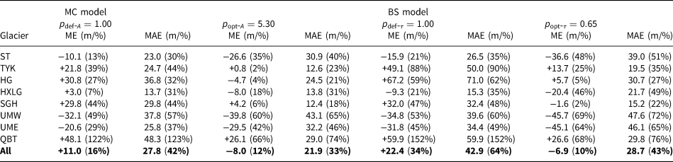
Table 2 lists the default and optimised parameters with corresponding mean error (ME) and MAE between measured and simulated ice thickness. The measured ice thickness used to calculate the ME/MAE is taken as a test group, and not used for model calibration. The optimised parameter of the MC model $p_{{\rm opt}\hbox{-} A} = 5.30$ means that the optimising ice creep parameter A is 5.3 times the default 2.4 × 10⁻²⁴s−1Pa−3, which improves the average MAE of all eight reference glaciers from 42 to 33% of average thickness. In the BS model, p opt−τ = 0.65 means 0.65 times the default τ (Eqn (3)). It decreases the average MAE from 64 to 43% of average thickness compared with the default τ. Both $p_{{\rm opt}\hbox{-} A}$
 and $p_{{\rm opt}\hbox{-} \tau }$
 indicate that our optimised parameters result in a lower ice thickness estimation than the default model settings. We noticed that the optimised runs result in higher MAEs (8–10% higher in the MC model, and 12–24% higher in the BS model) than the default runs for glaciers ST, UME and UMW. These thicknesses were already underestimated with the default parameters, and the regional optimisation leads to further underestimation. However, these values are compensated by a decreasing MAE in other glaciers (11–49% for MC and 26–76% for BS). Despite the estimated ice thickness produced by optimised parameters being 10–12% lower than the measurements (see Discussion for the possible reason for the underestimate), they still show a decrease of 4–24% absolute ME compared with the default parameters.
Table 2. Mean error (ME) and mean absolute error (MAE) between measured and simulated ice thickness for the reference glaciers with the mass conservation (MC) and basal shear stress (BS) models running with the default (p def) and optimised parameters (p opt)
Total ice volume and uncertainty
Figures 6a–b show the glacier flowlines and simulated section ice thickness based on the GAMDAM v2-SRTM for South Inylchek Glacier and Tomur Glacier as an example. The total ice volume in the Tian Shan is estimated to be 661.0 ± 163.5 km3 (area-averaged 56.6 ± 14.0 m) in the MC model and 552.8 ± 85.3 km3 (area-averaged 47.3 ± 7.3 m) in the BS model. These estimates are based on the GAMDAM v2 glacier outline and SRTM surface topography, and therefore represent the ice thickness of the year 2000. For glaciers in China, the simulated ice volume is 341.5 ± 112.2 km3 in the MC model and 284.7 ± 46.2 km3 in the BS model. For glaciers in other countries, the simulated ice volume is 319.5 ± 59.9 km3 in the MC model and 268.1 ± 59.5 km3 in the BS model. Small glaciers contribute to glacier numbers and area, but large glaciers dominate the ice volume. Glaciers with an area over 10 km2 account for <30% of the total glacier area, and for ~52% of the total ice volume (Fig. 7). The volume of the seven large glaciers with an area over 100 km2 is 145.4–211.7 km3 (26–32% of the total ice volume).

Fig. 6. Simulated section ice thickness and glacier flowlines (a–d), and the difference in distributed ice thickness (e and f, subtract the GAMDAM v2 ice thickness from the RGI v6 ice thickness) on the two largest glaciers in the Tian Shan. The left column (a, c and e) is from the mass conservation (MC) model, and the right column (b, d and f) is from the basal shear stress (BS) model. Figures a and b are based on the GAMDAM v2 glacier outline, c and d are based on the RGI v6 glacier outline. The SRTM is used in all of the simulations.

Fig. 7. Glacier area (grey bars), number (bold number) and ice volume (coloured bars) corresponding to the glacier area range.
According to the LOOCV approach, the calibration parameter p in the MC model ranges from 1.93 to 6.18 which results in ±154.2 km3 σ M (23% of total ice volume), and p in the BS model ranges from 0.61 to 0.71 and yields ±84.6 km3 σ M (15% of total ice volume). σ DEM is very limited in both the MC and BS models (~2% of the total ice volume). The overall σ GI of all glaciers in the Tian Shan is 8 and 2% of the total ice volume in the MC and BS models, respectively. While comparing glaciers in sub-regions, σ GI is 25% of the ice volume for glaciers in China (8% in other countries) in the MC model, and 17% of the ice volume for glaciers in China (lower than 1% in other countries) in the BS model. The ice volume range in the different glacier areas is mainly influenced by glaciers with an area over 10 km2 because of the significant ice volume uncertainty in the glacier inventory in China. For these glaciers, the RGI v6 results in a 42 and 28% overestimation compared with the GAMDAM v2 in the MC and BS models, respectively (Fig. 7).
Projection of future glacier mass
Based on our optimised ice creep parameter A and two glacier inventories, we project glacier mass change in the 21st century using the OGGM. The model is driven by the newest CMIP6 GCM climate dataset under four emission scenarios (SSP 1-2.6, SSP 2-4.5, SSP 3-7.0 and SSP 5-8.0) with 13–15 GCMs available for each scenario.
Our projection indicates that by the middle of the 21st century the remaining ice mass (relative to 2018) in the Tian Shan will be 70 ± 4% under SSP1-2.6 emission scenarios and 66 ± 4% under SSP5-8.5 emission scenarios, respectively (Fig. 8a, GAMDAM v2 estimate). By the end of the 21st century, the remaining ice mass in the Tian Shan will be 40 ± 4% under SSP1-2.6, 33 ± 3% under SSP2-4.5, 28 ± 3% under SSP3-7.0 and 22 ± 4% under SSP5-8.5 (Fig. 8a, GAMDAM v2 estimate). Considering the significant difference in the ice volume estimate between the GAMDAM v2 and RGI v6 for glaciers in China and in other countries, we also compared the ice mass change in those two subregions. While there is no obvious difference between the RGI v6 and the GAMDAM v2 relative ice mass change curve at the regional level, the differences are stronger for glaciers in China and in other countries. Both the absolute glacier mass (Figs 8e, f) and the annual mass loss (Figs 8h, i) show a greater difference between the RGI v6 and GAMDAM v2 for glaciers in both China and other countries. Compared with the GAMDAM v2, the RGI v6 shows a 19.8 ± 2.3 km3 (SSP1-2.6), 24.0 ± 1.6 km3 (SSP2-4.5), 27.5 ± 1.7 km3 (SSP3-7.0) and 30.4 ± 2.5 km3 (SSP5-8.5) greater ice mass loss in glaciers in China by the end of the 21st century, and less ice mass loss for glaciers in other countries: 15.7 ± 1.7, 19.0 ± 1.4, 21.9 ± 1.7 and 24.7 ± 2.3 km3.

Fig. 8. Glacier mass (relative to 2018, a–c), glacier mass (in km3, d–f) and annual mass loss (in km3, d–f) projection. The left column (a, d and g) shows the result for all the Tian Shan glaciers, the middle column (b, e and h) shows the result for glaciers in China and the right column (c, f and i) shows the result for glaciers in other countries. The shading indicates ± 1 std dev. for the GAMDAM v2 run (SSP1-2.6 and SSP5-8.5 are shown for clarity).
Discussion
Comparison with previous research
Figure 9 shows the simulated ice thickness compared to observations for our two inverse models and the five estimates from Farinotti and others (Reference Farinotti2019). For the glaciers present in the GlaThiDa v2 (ST, SGH, UME and UMW), which was used by Farinotti and others (Reference Farinotti2019), our results tend to underestimate ice thickness. While our estimation shows less bias for the glaciers new to the GlaThiDa v3 (TYK, HG, HXLG and QBT) than Farinotti and others (Reference Farinotti2019). This is because the newly added glaciers cover larger areas and were given more weight, and therefore have more influence on the model parameters. Comparing the simulated thickness in Farinotti and others (Reference Farinotti2019) with observed measurement thickness, the exceptionally good performance of their Model 4 (F4 in Fig. 9) for the glaciers included in the GlaThiDa v2 is notable and due to having used data assimilation during the calibration procedure. We did not find a better performance for their Model 4 compared to their other three models (hereafter, Models 1–4 in Farinotti and others (Reference Farinotti2019) are referred to as Model 1–4) in the newly added glaciers. Overall, the MAE between simulated thickness and measured thickness for the eight reference glaciers is 33–43% (Table 2) in our two optimised models, which is lower than the 49–64% MAE of Farinotti and others (Reference Farinotti2019).

Fig. 9. The simulated ice thickness bias for mass conservation (MC), basal shear stress (BS) and the estimate (FC, F1, F2, F3 and F4) in Farinotti and others (Reference Farinotti2019). The bias for MC and BS is from simulation of the glacier outline (2013)/COPDEM. The bold glaciers are the newly added glaciers in the GlaThiDa v3, which were not used in Farinotti and others (Reference Farinotti2019). FC is the composite result, and F1–4 (Model 1–4 in Farinotti and others (Reference Farinotti2019)) are the single model estimates. The black dotted lines show the position of zero bias. The box notes the error range between the 25th and 75th percentiles, and the dashed line in the box shows the median. The whiskers indicate the farthest data points within 1.5 times the interquartile range. The crosses represent the outliers.
Compared with the estimates of Farinotti and others (Reference Farinotti2019), our estimated ice volume with the BS model is close to Model 4 (568.4 km3; following Fürst and others (Reference Fürst2017)), but 31% lower than Model 1 (802.5 km3; following Huss and Farinotti (Reference Huss and Farinotti2012)), 22% lower than Model 2 (715.2 km3; following Frey and others (Reference Frey2014)), 35% lower than Model 3 (854.1 km3; following Maussion and others (Reference Maussion2019)), and 24% lower than the composite result (727.7 km3). Compared with the previous volume-area scaling estimate, our results are 36–42% lower (GAMDAM v2 area) than the relationship V = 0.034 S 1.375 presented in Bahr and others (Reference Bahr, Meier and Peckham1997), and 34–41% lower (GAMDAM v2 area) than the relationship V = 0.043 S 1.29 presented in Grinsted (Reference Grinsted2013).
We believe that there are two main reasons why our estimates are lower than most of those in Farinotti and others (Reference Farinotti2019). The first is the updated model parameters, which are assumed to be improved thanks to the regional calibration and the additional observational data. For example, the estimates (based on the RGI v6) of Model 3 (OGGM) in Farinotti and others (Reference Farinotti2019) are 19% higher than our estimates (also based on the OGGM and RGI v6). The second is related to the glacier inventories: improvements in the GAMDAM v2 lead to an area increase in other countries, but the RGI v6 still has a larger area than the GAMDAM v2 in China. Altogether, the outcome is a reduction of the estimated volume.
We found that there are some homogeneous bias patterns between the simulated and the measured ice thickness for the models in Figure 9. For example, almost all of the models showed an underestimation for reference glaciers UMW and UME, but an overestimation for TYK, HG and QBT. There are some indications that these might be related to the type of climate or glacier. Huang (Reference Huang1990) classified Urumqi No. 1 Glacier (UME and UMW in our study; they used to be the two branches of the glacier before 2000) as an extra-continental glacier, and SGH and HG were classified as sub-continental glaciers. Comparing the simulated ice thickness bias of these glaciers (Fig. 9), UME and UMW show a higher but negative bias while SGH shows a slightly positive bias. Both TYK and ST are located to the west of Peak Tomur. Whereas TYK has a higher estimate in all of the models than ST. Similarly, the climate in TYK is more humid than in ST. The multi-annual precipitation from 1972 to 1990 was reported as 1139 mm (Bolch, Reference Bolch2007), while <400 mm from 1997 to 2014 in ST (Kronenberg and others, Reference Kronenberg2016). In Figure 9, the overestimation at HG was close to or even higher than QBT in the composite result and in Models 2–3 particularly. However, if we compare the simulation bias with the average measured thickness, the highest average simulation bias is <60% of the average measured thickness in HG, but near or even over 100% of the average measured thickness for most of the models in QBT. Wang and others (Reference Wang, Li, Li, Wang and Wang2011) suggested that the characteristics of ice-velocity and glacier change of QBT are closer to a monsoonal maritime glacier, despite its location being far from the ocean. In addition, our optimised parameters generate a 10–12% negative ME, which is higher than the other regional research (with a ME near 5% of the mean measured ice thickness) in the Columbia River basin and the Austrian Alps (Helfricht and others, Reference Helfricht, Huss, Fischer and Otto2019; Pelto and others, Reference Pelto, Maussion, Menounos, Radić and Zeuner2020).
Following most other research (e.g. Farinotti and others, Reference Farinotti, Huss, Bauder, Funk and Truffer2009a, Reference Farinotti, Huss, Bauder and Funk2009b; Frey and others, Reference Frey2014; Pelto and others, Reference Pelto, Maussion, Menounos, Radić and Zeuner2020; Millan and others, Reference Millan, Mouginot, Rabatel and Morlighem2022), we applied a ‘one-size-fits-all’ parameter strategy to estimate the ice thickness in the entire Tian Shan range. However, considering the high model bias, the parameter strategy needs to be improved if more data are available. The homogeneous bias pattern which we mentioned in the above paragraph might give us insight on how to connect the model parameter with climate/glacier type. For example, combining it with remote-sensing technology (e.g. inversion of ice temperature, precipitation and velocity), optimizing the parameter for smaller regions with more homogeneous glaciers, or quantitatively analysing the relation between A and τ with climate. It should be noted that the homogeneous bias might also result from the glacier size, shape, topography, mass balance profile and so on. To take these into account, some statistical models (e.g. Bayesian inference used in Werder and others (Reference Werder, Huss, Paul, Dehecq and Farinotti2020) and Rounce and others (Reference Rounce, Hock and Shean2020)) or neural network/machine learning models are expected to improve the model performance in the future. Another promising aspect is combining the 3-D high-order numerical ice model with the 1-D flowline model. The 3-D high-order numerical ice model could take more factors (e.g. ice velocity, ice temperature) into account and describe the physical characteristics of the reference glacier with a high degree of accuracy, and the 1-D flowline model could be trained with the result of the 3-D high-order numerical ice model.
The influence of glacier outlines and the DEM
Our optimised parameters were determined using the DEM and glacier outline around 2013. The measured ice thickness was surveyed between 2008 and 2014. Strictly speaking, our optimised parameters only reflect the glacier status at the survey date of these data. However, the survey dates of the GAMDAM v2 were between 1994 and 2008 (Fig. 4), and the SRTM only represents the topography in 2000. Here we use the elevation change research of Hugonnet and others (Reference Hugonnet2021) to carry out a simple qualitative analysis to show the response of our inverse model to glacier change. We run the inverse models with the glacier outlines (2013)/COPDEM and glacier outlines (2000)/SRTM input combination to calculate the ice volume in 2013 and 2000 for the seven reference glaciers (excluding QBT). Then the ice volume difference between 2013 and 2000 is converted to annual thickness change rate (m a−1) for comparison with the elevation change rate in Hugonnet and others (Reference Hugonnet2021).
The result shows that the ice volume difference converted to annual thickness change rate is −0.42 m a−1 in the MC model, which agree with the elevation change rate (−0.59 ± 0.36 m a−1) during 2000–2010 in Hugonnet and others (Reference Hugonnet2021). While for BS model, the annual thickness change rate is only −0.12 m a−1 and obviously less than the absolute value of elevation change rate in Hugonnet and others (Reference Hugonnet2021). In fact, the reason that the MC model shows more mass loss than the BS model in the 2000–2013 simulation is that it is more sensitive to changes in glacier area. Comparing the ice volume between the glacier outlines (2013)/SRTM and the glacier outlines (2000)/SRTM input combination, the converted annual thickness change rate is −0.41 m a−1 in the MC model and 0.23 m a−1 in the BS model. While the ice volume difference converted to annual thickness change rate between the glacier outlines (2000)/COPDEM and the glacier outlines (2000)/SRTM input combination is ~−0.05 m a−1 for both the MC and BS models. The difference in all of these ice volumes converted to annual thickness change rate is quite limited compared with the vertical uncertainty of DEMs (16 m for SRTM and 4 m for COPDEM).
The high sensitivity of the MC model to glacier area change is also reflected in the simulated ice volume difference (σ GI) based on the GAMDAM v2 and the RGI v6. The most significant volume difference between the GAMDAM v2 and the RGI v6 result is in glaciers with an area over 10 km2 (Fig. 7). It is interesting that the RGI v6 results in a larger ice volume than the GAMDAM v2 for glaciers in China, while it is the opposite for glaciers in other countries. This is consistent with the glacier area differences between the two glacier inventories.
The MC model is more sensitive to area than the BS model because its estimate of ice thickness is based on ice flux. A larger glacier area, especially a larger accumulation region, means more ice flux through a cross-section, and also results in greater ice thickness or ice volume. In the BS model, however, ice thickness is mainly determined by τ and α. Whereas the maximum τ is limited to $p_{{\rm opt}\hbox{-} \tau } \times 150\,{\rm kPa}$ for glaciers with an elevation range over 1.6 km. A good example of this is the South Inylchek Glacier. The area of South Inylchek Glacier is 373.6 km2 in the RGI v6 and 473.9 km2 in the GAMDAM v2. There is no obvious difference for the flowlines, especially main flowlines, between the RGI v6 (Figs 6c, d) and GAMDAM v2 (Figs 6a, b). While the MC model results in a distinctly higher thickness in the middle part of main flowlines in the GAMDAM v2 (Fig. 6a) than the RGI v6 (Fig. 6c), which is the result of ice flux increasing with glacier area. In contrast, the BS model shows less difference in thickness in the same region (Figs 6b, d), since in both RGI v6 and GAMDAM v2, the basal shear stress τ of the glacier reaches the maximum value.
Except for glacier volume, different glacier areas might also have a significant influence on ice distribution in the OGGM, by changing the route of the automatically extracted flowlines. For the South Inylchek Glacier, there is not a clear difference between the RGI v6 and GAMDAM v2 glacier flowline (Figs 6a, c). Whereas Tomur Glacier shows a completely different situation, especially for the main flowline. The RGI v6 glacier outline results in a quite convoluted and unrealistic main flowline in this glacier. In the MC model, the main flowline receives the ice mass transformed from the other tributary branch, which results in a greater ice flux and thickness. Therefore, ice thickness in the south-east part of Tomur Glacier (annotated as ‘Positive difference’ in Fig. 6e) in the RGI v6 simulation is significantly thicker than that in the GAMDAM v2 simulation. But ice thickness simulated using the RGI v6 glacier outline is significantly thinner than when using the GAMDAM v2 glacier outline in the centre of the Tomur Glacier (annotated as ‘Negative difference’ in Fig. 6e). While at the lower end of the Tomur Glacier (annotated as ‘Less difference’ in Fig. 6e), the main flowlines for the RGI v6 and the GAMDAM v2 are almost coincident, and all of the upper stream ice fluxes come together. Therefore, there is a very small difference in the ice thickness in the RGI v6 and the GAMDAM v2 simulations. However, in the BS model, ice thickness is only determined by the ice surface slope for glaciers with an elevation difference over 1.6 km (see Eqns (1) and (2)). The different flowline traces will influence the ice surface slope, but it is clear that the influence on ice thickness distribution is limited (Fig. 6f).
Uncertainty of the ice thickness estimate
Huss and Farinotti (Reference Huss and Farinotti2012) indicated that the influence of the glacier outline on ice thickness estimates might be significant. Farinotti and others (Reference Farinotti2019) attributed their estimate being lower than other studies to the difference between the inventories. In our study, the ice volume difference between inventories is only 2–8% (depending on the approach) of the estimated ice volume of the entire Tian Shan range. This is because the representation of glacier area in the inventories shows a marked contrast between glaciers in China and in other countries, which is a coincidence for this region, and these differences may not compensate one another in other regions. For glaciers in the sub-regions, the maximum difference reaches 17% for the BS model and 25% for the MC model, which is equal to or even higher than the uncertainty caused by the model parameters. In contrast, the choice of DEM shows a quite limited influence, which agrees with Pelto and others (Reference Pelto, Maussion, Menounos, Radić and Zeuner2020) and Ramsankaran and others (Reference Ramsankaran, Pandit and Azam2018).
The estimated ice volume difference between models is 108.2 km3 (16–19% of the ice volume, depending on approach), which is in the range in Farinotti and others (Reference Farinotti2019). Our MC model estimate agrees with that of the BS model within its uncertainty range, but the BS estimate does not. This may indicate that the MC model overestimates ice volumes, or that the BS model uncertainty estimates are too low. Pieczonka and others (Reference Pieczonka, Bolch, Kröhnert, Peters and Liu2018) optimised their ice thickness inverse model based on measured ice thickness and estimated the ice thickness of four large glaciers (over 50 km2) by taking into account ice surface velocity and basal sliding. Here, we compare our estimated ice volume with their estimate and the estimates in other work listed in their study (Fig. 10). The BS model estimate is very close to that of Pieczonka and others (Reference Pieczonka, Bolch, Kröhnert, Peters and Liu2018). In contrast, the MC model still shows an overestimate, despite the estimated ice volume being closer to that of Pieczonka and others (Reference Pieczonka, Bolch, Kröhnert, Peters and Liu2018) than the other result listed in their study. The reason for the overestimate may be related to basal sliding. Following Pelto and others (Reference Pelto, Maussion, Menounos, Radić and Zeuner2020), we assume that there is no basal sliding and transferred the uncertainty to ice creep parameter A. Since our reference glaciers are significantly thinner than the four large glaciers, the optimised parameter A might be underestimated for these glaciers, considering a greater ice thickness corresponding to a higher basal sliding velocity under the same ice creep parameter A (see Eqns (4) and (5) in Maussion and others, Reference Maussion2019). Very few studies of Asian glaciers have measured basal sliding directly, but some studies have provided a minimum estimate by comparing remotely-sensed winter and summer surface velocities (Benn and others, Reference Benn2017). Assuming there is no basal sliding in winter, the contribution of basal sliding to glacier surface velocity is ~32% for the maritime glaciers in the south-eastern Tibetan Plateau (Wu and others, Reference Wu2019), which is close to that of Kaxkar Glacier (33%) in the Tian Shan (Li and others, Reference Li2014), while it is significantly lower than that at the flat terminus in Kaxkar and South Inylchek Glacier (86–99%) estimated by Pieczonka and others (Reference Pieczonka, Bolch, Kröhnert, Peters and Liu2018). In the MC model, an 85% (33%) contribution of basal sliding to surface velocity will result a 35% (10%) decrease in ice thickness. It is necessary to reduce the uncertainty of basal sliding and take it into account in the MC model in future.

Fig. 10. Comparing mean ice thickness in the glaciers in Pieczonka and others (Reference Pieczonka, Bolch, Kröhnert, Peters and Liu2018). P2018 is the estimate of Pieczonka and others (Reference Pieczonka, Bolch, Kröhnert, Peters and Liu2018); $\overline {h_{{\rm Huss}}} , \;\overline {h_{{\rm Lins}}}$ and $\overline {h_{{\rm su}}}$
 are the cases compared in Pieczonka and others (Reference Pieczonka, Bolch, Kröhnert, Peters and Liu2018) following the methods of Huss and others (Reference Huss and Farinotti2012), Paul and Linsbauer (Reference Paul and Linsbauer2012) and Su and others (Reference Su, Ding and Liu1984), respectively. All of the data are from Table 6 in Pieczonka and others (Reference Pieczonka, Bolch, Kröhnert, Peters and Liu2018), except for mass conservation (MC) and basal shear stress (BS).
Glacier mass projection
In our relative glacier mass projection, the ice thickness difference between inventories is the opposite for glaciers in China and in other countries, but the glacier mass difference between inventories is consistent (Figs 8b–c). For glaciers in China, a higher ice volume estimate from the RGI v6 corresponded to higher relative glacier mass remaining at a certain point in time than the estimate from the GAMDAM v2 (Fig. 8b), which agrees with Farinotti and others (Reference Farinotti2019). However, for glaciers in other countries, a lower ice volume estimate from the RGI v6 also results in a higher retention of glacier mass (Fig. 8c). This is because the difference between the RGI v6 and the GAMDAM v2 in other countries is mainly focused on the headwall regions (see the Data and methods sections), which are normally located at a higher altitude compared with other glacier areas, and therefore less prone to melt. Moreover, the range between inventories is quite limited in our study compared with Farinotti and others (Reference Farinotti2019). This may be due to the following two aspects: (1) the difference in ice volume estimates (25 and 8% for glaciers in China and in other countries, respectively) between inventories in our study is clearly less than the difference (35% for glaciers in Central Asia) in Farinotti and others (Reference Farinotti2019) and Huss and Farinotti (Reference Huss and Farinotti2012); (2) the difference between the RGI v6 (used in Farinotti and others (Reference Farinotti2019)) and the RGI v2 (used in Huss and Farinotti (Reference Huss and Farinotti2012)) might be greater than between the GAMDAM v2 and the RGI v6, considering the many missing glaciers, undifferentiated glacier complexes, unmatched geolocation in the RGI v2 (Farinotti and others, Reference Farinotti2019).
Despite the difference in the relative glacier mass projection between inventories being quite limited, the absolute glacier mass loss does matter since the local water supply is highly dependent on it. During the simulation periods (2018–2100), the difference of total absolute mass loss between the RGI v6 and GAMDAM v2 ranges from 19.8 ± 2.3 km3 (SSP1-2.6) to 30.4 ± 2.5 km3 (SSP5-8.5) in China and from 15.7 ± 1.7 km3 (SSP1-2.6) to 24.7 ± 2.3 km3 (SSP5-8.5) in other countries, which is higher than the difference between the adjacent emission scenarios, for example, the 18.0 ± 7.1 km3 difference (mean of GCMs) between SSP1-2.6 and SSP2-4.5 and the 11.7 ± 5.1 km3 (mean of GCMs) difference between SSP3-7.0 and SSP5-8.5 (both for GAMDAM v2 projection in China).
During the last decade, ~40% of glacier ablation could not be compensated by accumulation in High Mountain Asia (Miles and others, Reference Miles2021). This part of glacier ablation makes a great contribution to alleviating regional water stress. Pritchard (Reference Pritchard2019) indicated that the imbalance in glacier melt input to the dam catchments can be nearly 60% for some rivers originating in the Tian Shan in a dry summer. Rounce and others (Reference Rounce, Hock and Shean2020) suggested that excess meltwater (mass loss in this study) drives the timing of peak water and plays a more important role for the westerlies-controlled river basin than areas controlled by the monsoon. For example, for the Tarim basin, the excess meltwater might contribute ~60% of annual glacier runoff during peak water (under RCP 8.5 emission scenario). The lower glacier mass loss projection based on the GAMDAM v2 indicates the basins (like Tarim) fed by the glaciers in China might encounter a higher drought stress than previous studies based on the RGI v6 glacier inventory.
Ten surging glaciers with a total area of 159.67 km2 (~1% of the glacier area in the Tian Shan) have been reported in the region between 1990 and 2019 (Zhou and others, Reference Zhou2021). The influence of surging on the calibration and inversion estimates is largely unknown, but we expect high uncertainties for these glaciers. Furthermore, the impact of debris cover has not been considered. While debris cover products have been developed recently (Herreid and Pellicciotti, Reference Herreid and Pellicciotti2020; Rounce and others, Reference Rounce2021), there are no available debris-cover masks for the GAMDAM v2. For the RGI v6, the uncertainty in debris-cover area between different studies is also significant. For example, Kraaijenbrink and others (Reference Kraaijenbrink, Bierkens, Lutz and Immerzeel2017) indicate that the glacier area covered by debris is ~11% (10 737 km2) of the total glacier area in the high mountains of Asia, which is 28% higher than in Scherler and others (Reference Scherler, Wulf and Gorelick2018) and 23% higher than Herreid and Pellicciotti (Reference Herreid and Pellicciotti2020). These differences in debris cover area might lead to a significant uncertainty for the ice thickness inversion and glacier mass projection. We expect the influence of debris cover to be strongest for the ice thickness inversion (by affecting the mass flux estimates), but the influence on projections is likely to be compensated by calibration (Compagno and others, Reference Compagno2022).
Conclusions
Our study simulated the ice thickness of glaciers in the Tian Shan range based on two glacier inventories (RGI v6 and GAMDAM v2), two DEMs (SRTM and COPDEM) and the GlaThiDa v3. The parameters of two flowline models following different methods (one for mass conservation and one for basal shear stress) were optimised by matching more than 13 000 ice thickness measurements in eight reference glaciers to improve model performance. The optimised models show a 33% MAE in the MC model and 43% MAE in the BS model, which are 9–21% lower than the default model parameters and 16–21% lower than the previous global estimate of Farinotti and others (Reference Farinotti2019). The ice volume for glaciers in the Tian Shan is estimated as 661.0 ± 163.5 km3 in the MC model and 552.8 ± 85.3 km3 in the BS model, which is 34–42% lower than the volume-area scaling estimate (Bahr and others, Reference Bahr, Meier and Peckham1997; Grinsted, Reference Grinsted2013) and 9–24% lower than the component estimate of Farinotti and others (Reference Farinotti2019). For the eight reference glaciers, the ice thickness of extra-continental glaciers tends to be significantly underestimated and tends to be substantially overestimated in maritime glaciers in both our research and Farinotti and others (Reference Farinotti2019).
Our analysis indicates that uncertainty about estimated ice thickness mainly originates from model parameter uncertainty over the entire Tian Shan, which might be 15–23% of the total ice volume. Glacier inventory is the next most important contributor, despite it being only 2 and 8% in the BS model and MC model for all of the Tian Shan glaciers. For glaciers in the sub-regions (in China and in other countries), the uncertainty could increase to 17–25% of the ice volume. The reason that glacier inventories show a quite limited contribution to the uncertainty of the entire Tian Shan estimate is that the glacier area difference between the RGI v6 and the GAMDAM v2 is compensated for by glaciers in China and in other countries, which is a coincidence. In addition, the MC model might overestimate the ice thickness in glaciers with an area over 50 km2, due to greater basal sliding than in small glaciers. Given the limited available data, our study could not fully investigate the influence of basal sliding, but this merits attention in future work.
Based on our ice thickness estimates and the two glacier inventories (RGI v6 and GAMDAM v2), we also projected future glacier mass. Our results show that the different ice thickness originating from the two glacier inventories will not have a significant influence on the future relative ice mass (relative to 2018). However, the GAMDAM v2 shows 30.4 ± 2.5 km3 less mass loss than the RGI v6 simulation for glaciers in China by the end of the 21st century under the highest CMIP6 emission scenario (SSP5-8.5). This reduced glacier mass loss might carry more risk for areas that are highly dependent on glacier meltwater, for example, the Ili River basin. This should also be given serious consideration in the future.
Data Availability
The datasets including the RGI v6, GAMDAM v2, SRTM DEM, COPDEM DEM and GlaThiDa v3 used in this study are freely available. All the code and reported glacier volumes are available at: https://github.com/Keeptg/Tian_shan_ice_volume_GoJ.
Acknowledgements
This work was supported by the Strategic Priority Research Program of the Chinese Academy of Sciences [grant No. XDA20060201], the National Natural Science Foundation of China [grant No. 41725001], the Second Tibetan Plateau Scientific Expedition and Research Program (STEP) [grant No. 2019QZKK0201] and the scholarship provided by the University of Chinese Academy of Sciences (UCAS). The simulations were run on the Climate Lab supercomputer, University of Bremen. We are grateful to the detailed comments and suggestions from Rijan Bhakta Kayastha and the other three anonymous reviewers, the Editorial Assistant, Lynsey Rowland, the Scientific Editor, Rakesh Bhambri, and the Chief Editor, Hester Jiskoot, which were of great help in improving the manuscript. We also thank the European space agency for the provision of COPDEM. Fei Li acknowledges Matthias Dusch and other OGGM contributors for their help during the development phase of the basal shear stress model. Fei Li is also thankful for the help and support from colleagues at the Department of Atmospheric and Cryospheric Sciences (ACINN), Innsbruck University, Austria and Miss Zhao, who helped him have a happy and fulfilling year even in the unusual year 2020.


 Open access