


Introduction
The mass wastage of the world's glaciers and ice caps is accelerating in many regions, and more than half of the glaciers outside Antarctica are projected to disappear under future warming scenarios (Fox-Kemper and others, Reference Fox-Kemper2021). The effect of these changes is impacting local communities and ecosystems, as well as coastal communities world-wide, that face displacement due to increased risk of coastal flooding and erosion caused by global sea level rise. In recent decades, the Greenland Ice Sheet (GrIS) and peripheral glaciers and ice caps (GICs) in Greenland have experienced a dramatic loss of mass in response to climate change (Bevis and others, Reference Bevis2019; Khan and others, Reference Khan2020; King and others, Reference King2020; Shepherd and others, Reference Shepherd2020; Fox-Kemper and others, Reference Fox-Kemper2021). Records from coastal and inland weather stations in Greenland show that the surface temperature has increased by between ~1.7 °C (summer) and ~4.4 °C (winter) in the period from 1991 to 2019 (Hanna and others, Reference Hanna2021). As a result, surface melting on the GrIS has reached levels that exceed those of the last 350 years (Fox-Kemper and others, Reference Fox-Kemper2021). In addition to changes in surface mass balance, dynamic losses caused by accelerating glaciers has contributed considerably to the total mass loss from the GrIS (Bevis and others, Reference Bevis2019; Khan and others, Reference Khan2020; King and others, Reference King2020). While the potential for total change is smaller for the GICs in Greenland, current mass loss is substantial and constitutes 13% of the total 266 ± 16 GT yr−1 lost from global glaciers (excluding the Greenland and Antarctic ice sheets) between 2000 and 2019 (Hugonnet and others, Reference Hugonnet2021). Accurate predictions of future change are paramount for sustainable mitigation and adaptation, and rely on precise estimates of climate conditions (Eyring and others, Reference Eyring2021), current thickness and volume of the world's glaciers (Farinotti and others, Reference Farinotti2019; Hock and others, Reference Hock2019; Welty and others, Reference Welty2020), and thorough model treatment of the dynamic processes controlling ice flow (Beckmann and others, Reference Beckmann2019; Shannon and others, Reference Shannon2019; Marzeion and others, Reference Marzeion2020).
While the importance of ice thickness measurements is not disputed, observations are currently limited to ~ 3 000 of the world's ~ 217 000 glaciers (Welty and others, Reference Welty2020). As a consequence, estimates of worldwide ice thickness distribution rely strongly on the performance of ice flow models (Farinotti and others, Reference Farinotti2019). In Greenland, NASA's Operation IceBridge has put significant efforts into mapping of the ice sheet (Paden and others, Reference Paden, Li, Leuschen, Rodriguez-Morales and Hale2010, updated 2021), while the ~ 20 300 GICs (Rastner and others, Reference Rastner2012) have received much less attention. In version 3 of the worldwide database for glacier thickness observations, Welty and others (Reference Welty2020) report that a total of 1 361 GICs in Greenland have at least one observation of ice thickness. However, most of these observations come from widely distributed profiles of airborne measurements (often several km apart) associated with measurements of the ice sheet, as presented for the Renland Ice Cap in East Greenland (Koldtoft and others, Reference Koldtoft, Grinsted, Vinther and Hvidberg2021). While these airborne measurements provide invaluable information on the GICs of Greenland, publications describing more targeted and ground-based measurements of ice thickness are limited to a mere eight GICs. These are: Qasigiannguit Gletsjer (Abermann and others, Reference Abermann, van As, Petersen and Nauta2014), Aqqutikitsoq Gletsjer (Marcer and others, Reference Marcer2017) and Kuannersuit Glacier (Yde and others, Reference Yde2019) in West Greenland, Roslin Gletsjer (Davis and others, Reference Davis, Halliday and Miller1973) and Mittivakkat Gletsjer in East Greenland (Knudsen and Hasholt, Reference Knudsen and Hasholt1999; Yde and others, Reference Yde2014), and Nunatarssuaq Ice Cap (Welty and others, Reference Welty2020), Qaanaaq Ice Cap (Sugiyama and others, Reference Sugiyama2014) and Hans Tausen Iskappe in North Greenland (Zekollari and others, Reference Zekollari, Huybrechts, Noël, van de Berg and van den Broeke2017). Calculations of volume change in recent decades and predictions for future conditions exist for several of these glaciers and illustrate that they are currently in severe climatic disequilibrium. Aqqutikitsoq Gletsjer lost ~26% of its volume between 1985 and 2014 (Marcer and others, Reference Marcer2017), and Mittivakkat Gletsjer lost ~29% between 1994 and 2012 (Yde and others, Reference Yde2014). Modelling experiments for the Hans Tausen Iskappe show that the glacier is particularly sensitive to climate change, and that ~80% of its volume will disappear in the future if air temperature and precipitation remain at 2005–2014 conditions (Zekollari and others, Reference Zekollari, Huybrechts, Noël, van de Berg and van den Broeke2017). Similar results were found by Larsen and others (Reference Larsen2017) for GICs in Kobbefjord, southwest Greenland, which are projected to disappear completely in ~30–90 years assuming a future retreat rate equal to that documented during the 21st century.
While information on ice thickness allows us to better quantify the potential for change and serves as baseline for distributed ice flow models, knowledge of the thermal regime of glaciers remains crucial to accurate predictions of current and future ice dynamics (Cuffey and Paterson, Reference Cuffey and Paterson2010; Irvine-Fynn and others, Reference Irvine-Fynn, Hodson, Moorman, Vatne and Hubbard2011). The importance of the thermal regime of glaciers to ice velocity is well documented and relies on an understanding of heat transfer at the glacier surface, englacially and at the ice base (Cuffey and Paterson, Reference Cuffey and Paterson2010). In a warming climate, factors influencing the thermal regime of glaciers have been identified as potential drivers of rapid changes in glacier dynamics and geometry (Phillips and others, Reference Phillips, Rajaram and Steffen2010, Reference Phillips, Rajaram, Colgan, Steffen and Abdalati2013; Vaughan and others, Reference Vaughan2013; Colgan and others, Reference Colgan, Sommers, Rajaram, Abdalati and Frahm2015; Dunse and others, Reference Dunse2015). For example, studies on the thermal regime of GrIS suggest that a change from cold (below pressure melting point) to temperate (at pressure melting point) conditions could occur as more surface melt is routed through conduits in the ice and the potential for englacial latent heat release by refreezing meltwater (cryo-hydrological warming) is increased (Phillips and others, Reference Phillips, Rajaram and Steffen2010, Reference Phillips, Rajaram, Colgan, Steffen and Abdalati2013; Colgan and others, Reference Colgan2011, Reference Colgan, Sommers, Rajaram, Abdalati and Frahm2015). Conversely, many smaller Arctic glaciers may currently be experiencing a thermal change from polythermal to completely cold conditions due to a loss of deep firn and consequently limiting refreezing of meltwater in these porous layers (Rippin and others, Reference Rippin, Carrivick and Williams2011; Karušs and others, Reference Karušs2022). The scale of spatial and temporal resolution required to model variability in glacier thermal regime constitutes an enormous challenge for glacier models and relies on accurate field observations (Aschwanden and others, Reference Aschwanden, Fahnestock and Truffer2016; Lampkin and others, Reference Lampkin2018; Aschwanden and others, Reference Aschwanden2019). The spatial complexity of thermal regime has been documented from borehole data (e.g. Lüthi and others, Reference Lüthi2015; Seguinot and others, Reference Seguinot2020) and measurements with ground penetrating radar (GPR) (e.g. Macheret and others, Reference Macheret2009; Wilson and others, Reference Wilson, Flowers and Mingo2013; Gilbert and others, Reference Gilbert2020; Karušs and others, Reference Karušs2022). However, so far, studies of thermal conditions in Greenland have focused on GrIS (e.g. Phillips and others, Reference Phillips, Rajaram, Colgan, Steffen and Abdalati2013; Harrington and others, Reference Harrington, Humphrey and Harper2015; Lüthi and others, Reference Lüthi2015; Hills and others, Reference Hills2018; Seguinot and others, Reference Seguinot2020) and little is known about the conditions of GICs (Sugiyama and others, Reference Sugiyama2014). By furthering our understanding of the thermal structures of glaciers and adding to the sparse dataset of ice thickness observations on Greenland GICs, the discrepancies observed both among various modelled responses and between model predictions and observations, can be reduced.
The aim of this paper is to elucidate the geometry and geothermal structure of Lyngmarksbræen Ice Cap, and to discuss the implications of these observations for future changes. Here, we present radar measurements of snow, firn and ice thickness using three different antenna frequencies. We interpolate ice-cap wide ice and snow thickness and use this to construct a map of bed topography beneath the ice and calculate the first volume estimate for Lyngmarksbræen Ice Cap. In addition, we map the distribution of temperate and cold ice along radar transects and show that zones of thick temperate ice are closely related to the upstream presence of surface crevasses. We discuss the significance of observed ice cap characteristics and hypothesise on how Lyngmarksbræen Ice Cap may change in a future warming climate. Overall, the results contribute data for the forcing and validation of dynamic ice flow models and demonstrate the need for complex treatment of heat transfer in glacier modelling studies.
Study Area
Lyngmarksbræen Ice Cap (69°19’N, 53°36’W) is located in the southwestern part of the island Qeqertarsuaq (formerly Disko Island) in the Disko Bay area of West Greenland (Fig. 1). The climate on Qeqertarsuaq island is polar maritime with a mean annual air temperature (1961–1990) of −4.0 °C in the town Qeqertarsuaq (formerly Godhavn), which is situated on the coast just south of Lyngmarksbræen Ice Cap (Humlum, Reference Humlum1999). The mean annual precipitation is approximately 400 mm water equivalent at sea level and the majority falls as snow (Humlum, Reference Humlum1999).
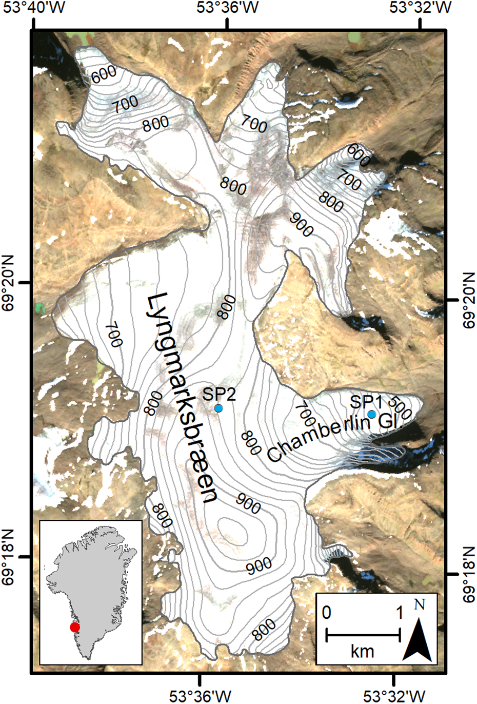
Figure 1. Sentinel-2B image of Lyngmarksbræen Ice Cap taken on 30 August 2016 with 20 m surface contour lines extracted from ArcticDEM v3.0 (Porter, Reference Porter2018) and corrected for the GGeoid16 gravimetric geoid model for Greenland (Forsberg, Reference Forsberg2016). The two blue dots indicate locations of pits dug for snow density measurements.
Lyngmarksbræen Ice Cap has six outlet glaciers, of which Chamberlin Gletsjer is the largest. In 1894, Chamberlin (Reference Chamberlin1894) initiated detailed mapping, photo documentation and descriptive surveys of the glacier. This work was continued in 1897 (Pjetursson, Reference Pjetursson1898), 1898 (Steenstrup, Reference Steenstrup1901), 1912 (de Quervain and Mercanton, Reference de Quervain and Mercanton1925) and 1923 (Froda, Reference Froda1925). More recently, Yde and Knudsen (Reference Yde and Knudsen2007) have used aerial photographs and satellite imagery to extend the glacier length record to 2005. The outlet glaciers from Lyngmarksbræen Ice Cap were still positioned at their Little Ice Age maximum in 1894 (Chamberlin, Reference Chamberlin1894; Yde and Knudsen, Reference Yde and Knudsen2007), but since then all have receded significantly. Between 1894 and 2005, Chamberlin Gletsjer receded 2.5 km (Leclercq and others, Reference Leclercq2014), which is equal to ~40% of its 1894 length. At the time of the radar fieldwork presented here (April 2017), Lyngmarksbræen Ice Cap covered an area of 20.2 km2 and surface elevations ranged between ~425 m a.s.l. and ~950 m a.s.l. (Fig. 1).
Glacier surging is a common phenomenon on Qeqertarsuaq island (Weidick, Reference Weidick1988; Yde and Knudsen, Reference Yde and Knudsen2007; Citterio and others, Reference Citterio, Paul, Ahlstrøm, Jepsen and Weidick2009), but none of the outlet glaciers from Lyngmarksbræen Ice Cap have been observed to surge or show distinct diagnostic features of past surge activity such as potholes, looped-medial moraines, or proglacial crevassed-squeezed ridges (Yde and Knudsen, Reference Yde and Knudsen2007). Nevertheless, glacier surging cannot be excluded as an explanation for extensive glacier advances during the Little Ice Age, and the advanced positions of the outermost ice-cored terminal moraines could suggest that some of the outlet glaciers have experienced glacier surging in the past, or that their ice dynamics are highly sensitive to climate variations (Yde and Knudsen, Reference Yde and Knudsen2007).
Lyngmarksbræen Ice Cap is important to the local community. Hunters and fishers arrange tourist dog sledging trips on the ice cap during the summer season and income from these activities provides a significant contribution to the Qeqertarsuaq economy. However, the viability of the glacier tours is threatened, as in recent years the ice cap has receded significantly at the southern ice margin and summer access to the ice has become problematic.
Ground penetrating radar measurements
The GPR fieldwork at Lyngmarksbræen Ice Cap was conducted using a range of antenna frequencies. GPR is the preferred method for mapping of ice thickness distribution (Welty and others, Reference Welty2020) and a powerful tool for investigations of snow thickness, internal layers, crevasses, meltwater channels and glacier thermal regime due to the level of detail and spatial coverage (e.g. Plewes and Hubbard, Reference Plewes and Hubbard2001; Dowdeswell and Evans, Reference Dowdeswell and Evans2004; Navarro and Eisen, Reference Navarro, Eisen, Pellikka and Rees2009; Bælum and Benn, Reference Bælum and Benn2011; Sevestre and others, Reference Sevestre, Benn, Hulton and Bælum2015; Gillespie and others, Reference Gillespie2017). The nature of the recorded electromagnetic signal provides important information on glacier characteristics. For example, crevasses are often recognised as vertically stacked diffraction hyperbolae (e.g. Navarro and Eisen, Reference Navarro, Eisen, Pellikka and Rees2009; Catania and Neumann, Reference Catania and Neumann2010; Colgan and others, Reference Colgan2016), and isolated englacial diffraction hyperbolae may result from meltwater channels and larger cavities (e.g. Travassos and Simões, Reference Travassos and Simões2004; Björnsson and Pálsson, Reference Björnsson and Pálsson2020). The level of detail observed in GPR measurements is frequency dependent, but in general, cold ice will present as largely transparent zones, whereas strong signal scattering or ‘noisy’ data occur in temperate regions because of the presence of water (e.g. Smith and Evans, Reference Smith and Evans1972; Watts and England, Reference Watts and England1976; Travassos and Simões, Reference Travassos and Simões2004; Macheret and others, Reference Macheret2009; Wilson and others, Reference Wilson, Flowers and Mingo2013). Due to the combined effect of scattering and an increased absorption of energy by water, GPR surveys on temperate glaciers have a decreased signal-to-noise ratio and consequently poor penetration depth (Navarro and Eisen, Reference Navarro, Eisen, Pellikka and Rees2009).
Fieldwork
The GPR survey of Lyngmarksbræen Ice Cap was carried out between 6th and 10th of April 2017, before the onset of melting and when the snowpack was expected to be at or near its maximum thickness. Most ice thickness measurements were collected using a ProEx Malå GPR with 50 MHz in-line Rough Terrain Antennas (RTA). In addition, we used an IceRadar Turn-Key System with 5 MHz antennas (Mingo and Flowers, Reference Mingo and Flowers2010) in regions where the bed reflection was absent in the initial 50 MHz measurements, either due to thick ice or poor radar penetration depth. A ProEx Malå system was applied with a 500 MHz shielded antenna for measurements of snow, firn and marginal ice (<30 m). The 50 MHz and 500 MHz antennas have set antenna separations of 4.2 m and 0.18 m, respectively, while a separation of 30 m between antenna midpoints was chosen for the 5 MHz antennas. The various radar systems were towed behind snow scooters travelling at velocities of 10–15 km h−1, depending on the conditions on the glacier surface. Measurements collected with the Malå GPR were stacked four times, while the IceRadar measurements were stacked 256 times. Stacked GPR measurements were collected every 0.1 s (500 MHz), 0.25 s (50 MHz) and 1 s (5 MHz) resulting in an average distance between ice and snow thickness observations of 0.3 m (500 MHz), 0.8 m (50 MHz) and 3.8 m (5 MHz). The 5 MHz IceRadar and 500 MHz Malå GPR were run simultaneously, with a minimum distance of 100 m between setups, and we observed no interference between the two radar systems during measurements. A total of ~131 km low frequency data (50 and 5 MHz) and ~43 km high frequency data (500 MHz) were collected along longitudinal and cross-glacier profiles, covering all accessible regions of the ice cap. GPS positions with a horizontal positioning accuracy of up to 5 m for the Malå GPR (G-Star IV BU-353S4 receiver) and 3 m for the IceRadar system (Garmin GPSx OEM sensor) were logged continuously during data collection, and coupled automatically with the GPR measurement.
In addition to GPR measurements, we dug snowpits on Chamberlin Gletsjer (SP1, 550 m a.s.l.) and further up-glacier near the ice cap plateau (SP2, 840 m a.s.l., Fig. 1). At both locations, we logged the vertical changes in snow densities at 30 cm intervals to enable calculations of radar wave velocity through the snowpack. Furthermore, to determine possible spatial variations in snow density away from the snow pits, manual snow depth soundings were conducted with avalanche probes at the start of each 500 MHz GPR profile (25 measurements in total). By combining observation from snow pits, manual snow depth soundings and high-frequency GPR profiling, snowpack characteristics were adequately mapped along survey tracks. However, measurements of ice thickness were prioritised during fieldwork, and high-frequency GPR measurements are sparsely distributed, except along Chamberlin Gletsjer.
Data processing
GPR data processing was conducted using the ReflexW module for 2D data analysis (Sandmeier Scientific Software, version 8.5), and included removal of low frequency signal (dewow), correction of time zero, accounting for large antenna separation for 5 MHz measurements (dynamic correction), gain application (energy decay or gain function) and F-K (Frequency-Wavenumber) migration (Stolt, Reference Stolt1978) to account for sloping bed topography. In addition to the described processing routine, a F-K filter had to be applied to the 500 MHz data to eliminate significant ringing, most likely caused by the proximity of the snow scooter. Following processing, we observed a strong basal reflector in all 5 MHz profiles and in most 50 MHz profiles. Clear reflections from the interfaces between snow, firn (when present) and the ice surface were observed in all 500 MHz profiles, along with glacier bed reflections in shallow regions (<30 m ice). The two-way travel time (TWT) to layer boundaries was determined using a manual (ice bed and temperate ice) and semi-automatic (ice surface) picking routine for all GPR profiles with visible reflectors.
The radio-wave velocity (RWV) of ice and snow varies with changes in the content of air and water (Hubbard and Glasser, Reference Hubbard and Glasser2005). Since the radar equipment used in this study does not allow for accurate common midpoint (CMP) measurements of RWV, an ice velocity of 168 m μs−1 was chosen for the conversion of TWT to depth, based on results reported by others on glaciers of similar temperature regime and thickness (Dowdeswell and Evans, Reference Dowdeswell and Evans2004; Navarro and Eisen, Reference Navarro, Eisen, Pellikka and Rees2009; Sugiyama and others, Reference Sugiyama2014). The RWV used for the time-to-depth conversion of snow and firn was found by using the empirical relationship described by Kovacs and others (Reference Kovacs, Gow and Morey1995) relating permittivity ($\varepsilon _r^{\prime}$ ) and density (ρ, kg m−3),

and subsequent calculations of RWV (v),

where c is the speed of light in vacuum. The average snow densities at SP1 (Chamberlin Gletsjer, 190 cm deep) and SP2 (upper plateau, 196 cm deep) were 358 kg m−3 and 370 kg m−3, respectively, which combined yield an average RWV for snow of 229 m μs−1. The snow depths derived from the calculated RWV and interpreted TWT compare well with the manual snow depth soundings collected at the start of each profile, suggesting only minor lateral variations in average snow density (±30 kg m−3) and hence RWV (±4.5 m μs−1). Measurements show that the firn layer is thin or absent in most surveyed regions, and consequently the combined snow and firn layer was assigned the RWV found for snow.
Interpolation maps
The point measurements of ice, snow and firn thickness were interpolated to produce maps that cover the entire Lyngmarksbræen Ice Cap. We conducted all interpolations in ArcGIS Desktop 10.6 using a combination of Radial Basis Functions (RBF) and Topo to Raster interpolation techniques. The RBF interpolation routine allows for RBF neighbourhood search division, which ensures that the interpolated values are based on measurements from more than one direction. This produces smoother and more realistic interpolations, particularly for GPR data that are concentrated along widely spaced profile lines. A search neighbourhood with four sectors and 45° offset were used for all RBF interpolations.
The map of combined snow and firn thickness was produced by interpolating between measurements using RBF (circular search neighbourhood) and letting the interpolation routine extend freely to the outline of the ice cap. A smoothing filter was applied to the RBF snow and firn thickness interpolation, after which contour lines for every 0.1 m depth increment were exported and manually corrected for interpolation artefacts. Finally, we used Topo to Raster to interpolate between corrected contour lines, to produce a 20 m grid sized map of combined snow and firn thickness.
To account for the expected valley topography beneath the outlet glaciers of Lyngmarksbræen Ice Cap, we chose a somewhat different interpolation routine for the ice thickness dataset. Firstly, the ice thickness measurements were supplemented with ice marginal values of zero thickness, extracted from a late summer Sentinel image (30th August 2016, Fig. 1). Subsequently, we determined the ice flow direction and outlet glacier catchment areas from a surface slope analysis of the ArcticDEM v3.0 (2018) provided by the Polar Geospatial Center. Based on this analysis, the ice cap was divided into four different regions characterised by similar ice flow axis (e.g. regions with ice flow in a western and eastern direction grouped together). Within each region, we applied an RBF interpolation routine with an ellipse search neighbourhood and the major axis aligned along the main ice flow axis. By applying an aligned ellipse search neighbourhood, we ensure that the interpolated values are influenced more strongly by measurements collected along upstream and downstream profiles. In addition, the influence of zero values along outlet glaciers margins is reduced. The individual regional interpolations compared well near catchment margins and were combined into one interpolation by applying a RBF interpolation across boundary data gaps of ~50 m. Interpolation artefacts were primarily found in regions without measurements, and to limit their influence on the final interpolation map, we exported 10 m ice thickness contours and the top 115 m contour line and used a low-pass filter to smooth them, before merging with a 0 m contour line delineating the glacier margin. Finally, we applied the Topo to Raster routine to interpolate between contour lines and produce the final 20 m grid sized interpolation of ice thickness. The ice thickness interpolation was corrected for the presence of snow and firn by accounting for the higher velocity in these layers. Finally, we subtracted the firn corrected ice thicknesses from the ArcticDEM (Porter, Reference Porter2018) to produce a 20 m grid sized map of the bed topography beneath Lyngmarksbræen Ice Cap. The bed topography was adjusted to sea level using the GGeoid16 gravimetric geoid model for Greenland (Forsberg, Reference Forsberg2016).
Error analysis
The magnitude of errors associated with the maps of snow and firn thickness, ice thickness and bed topography depend partly on the quality of the point measurements of snow and ice. The data quality is affected by errors in the applied RWV, inaccuracies when picking TWT to reflectors, and positioning errors of the individual radar measurements (Lapazaran and others, Reference Lapazaran, Otero, Martín-Español and Navarro2016). In addition to the measurement errors, inaccuracies in the produced maps arise from the complicated interpolation of layer thicknesses from an unevenly distributed dataset, and inherent errors in surface DEM (bed topography only). Below we describe the errors associated with the results in more detail.
Snow and firn thickness errors
Errors in the calculated RWV for snow arise from lateral variation in the snowpack density. Small discrepancies were observed between the snow depth probed during fieldwork and the depth observed in the GPR data, suggesting a velocity uncertainty for the snowpack of ~2%. This uncertainty increases in regions where a firn layer is present, as the RWV in the more compact firn layer will be lower than that measured for the snowpack (Hubbard and Glasser, Reference Hubbard and Glasser2005). The combined error in point measurements caused by inaccuracies in positioning and reflector picking can be estimated from a crossover analysis, where thicknesses found at intersecting GPR profiles are compared (e.g. Bamber and others, Reference Bamber2013; Farinotti and others, Reference Farinotti, King, Albrecht, Huss and Gudmundsson2014; Kutuzov and others, Reference Kutuzov, Thompson, Lavrentiev and Tian2018). The 500 MHz dataset intersects at 30 points, and a comparison of the interpreted snow and firn thicknesses at these locations show a maximum difference of 0.3 m and an average absolute difference of 0.1 m (0.07 m std dev). This constitutes an average absolute difference of 5.4% when expressed in relation to the local snow and firn thickness.
Measurements of snow and firn thickness are sparse apart from those on the Chamberlin Gletsjer, and it is difficult to quantify the interpolation error. However, variations in observed layer thickness across the ice cap are minor and the measured values may consequently provide good estimates of the unsurveyed regions of the ice cap. The magnitudes of such errors are not investigated further, as any error in the relatively thin snow and firn layer is unlikely to have any major impact on the ice thickness values, which is the focus of this study.
Ice thickness errors
The RWV for the ice at Lyngmarksbræen Ice Cap is unknown and a single RWV for ice was used for the entire ice cap, after which the presence of a snow and firn layer was accounted for. A RWV error of ~2% is reported in other studies using GPR measurements that have been adapted to local snow, firn and/or hydrothermal conditions (Navarro and others, Reference Navarro2014; Lapazaran and others, Reference Lapazaran, Otero, Martín-Español and Navarro2016). A water content of 1–2% will result in a lowering of the ice velocity of between 5 and 9 m μs−1 (Pettersson and others, Reference Pettersson2011), which for 50 m of temperate ice would amount to a ~2.5 m overestimation of the ice thickness. However, cold ice dominates the ice column in most regions of the Lyngmarksbræen Ice Cap, and we believe the overall inaccuracy of assigning a constant RWV is minor. When applied in ideal conditions, the low-frequency radar systems have a frequency dependent vertical resolution of ¼ of the signal wavelength and ranging from 0.8 m (50 MHz) to 8.4 m (5 MHz) in ice. To further assess the inaccuracy related to positioning and picking of the ice thickness measurements, we compared the interpreted ice thicknesses at 254 points where GPR profiles intersect. Results show a maximum difference of 8.8 m and an average absolute difference of 2.2 m (1.8 m std dev), which equals an average absolute difference of 5.2%, when expressed in relation to the local ice thickness.
As the potential for error is large for the ice thickness interpolation, the magnitude of the interpolation error was investigated more thoroughly. First, the fit of the 20 m grid sized interpolation to measurements was evaluated by comparing ice thicknesses at known locations across the ice cap (GPR measurements and glacier outline). The analysis shows a maximum difference between interpolation and observations of 19.2 m, an average absolute difference of 2.1 m and a 1.9 m std dev. The largest observed inaccuracies primarily relate to interpolation issues near the glacier boundaries, and given the 20 m interpolation grid size, the map generally reflect the measured ice thicknesses well.
To quantify the error of the ice interpolation routine at increasing distance from known points, we used generalised least squares (GLS) regression modelling to predict error at given distances from GPR profiles on the largest western outlet glacier (Fig. 2a). The predicted relationships between distance to known ice thickness and interpolation error were then used to create an error map for the entire ice cap. All statistical modelling was conducted in the R programming environment version 3.5.3 (R Core Team, 2019), using the gls function of the nlme library (Pinheiro and others, Reference Pinheiro, Bates, DebRoy and Sarkar2018). We envisioned two scenarios of uncertainty in the unsurveyed regions of the ice cap: (S1) areas where the interpolation routine relied mainly on input measurements from GPR profiles, and (S2) areas that were located between measured profiles and the ice margin. To investigate errors within these scenarios separately, we first created two subsets of measurements to use as ‘training data’. In creating these datasets, the area investigated by model S1 includes a northern boundary at the glacier margin, and the area of model S2 is bounded on three sides by the margin. Therefore, to investigate the possibility of greater inaccuracies close to the edge of the glacier, we generated an additional categorical variable where the data points were categorised according to whether they were closest to the glacier outline (‘O’) or to an included measured point (‘M’). This resulted in a large imbalance between O and M data points for S1. Therefore, only data points closest to input measured points were used, and the error close to the glacier boundary was not estimated. However, as there was a good balance between O and M data points for S2, we included this categorical variable as an extra predictor in the S2 regression model.
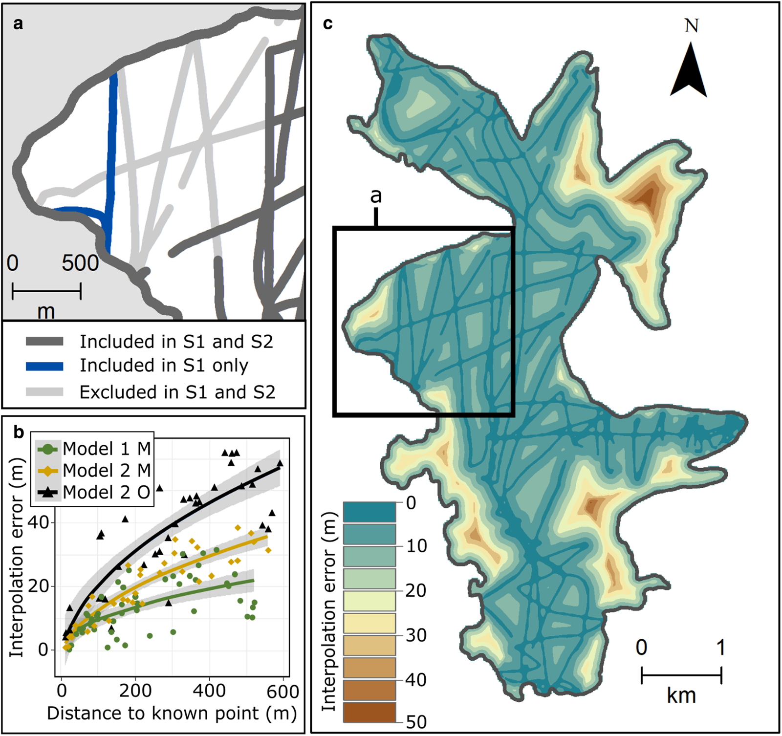
Figure 2. (a) Overview of GPR profiles included and excluded to create two subsets of data representing two scenarios (S1 = a scenario of an unsurveyed region where interpolated values rely mainly on surrounding measurements, S2 = a scenario where an unsurveyed region lies between measurements and the glacier margin). In each scenario, the difference between known thickness measurements and interpolated thickness was calculated (interpolation error). Interpolation errors for S1 were used in Model 1. Errors for S2 were used in Model 2; (b) the relationship between interpolation error and distance to known (measured) profile points. Solid lines are regression lines from generalised least squared models parameterised using square-root transformed variables. Predictions have been back-transformed to original units. Shading represents 95% confidence intervals. O = data points categorised as closest to glacier margin, M = data points closest to a measurement profile; (c) Interpolation error map using predictions from the regression models.
For each of these subsets, we made new RBF interpolations of ice thickness, and then calculated the difference between the excluded (observed) measurements and the interpolation at the corresponding points. This difference represents the interpolation error at each measurement point. We used these interpolation error values as response variable in two GLS regression models (one for each scenario), with distance from the nearest known (included) GPR profile point as explanatory variable. Both variables were square root transformed to normalise model residuals and achieve homogeneity of variance and predictions were back-transformed for plotting purposes.
GLS regression allows for the inclusion of spatial correlation structures to account for spatial autocorrelation in the data (i.e. data points close together are likely to violate the assumption of data independence). However, when using all available data points in the subsets, the models still retained some high residual spatial autocorrelation, according to Moran's I (Cliff and Ord, Reference Cliff and Ord1981). Therefore, we further reduced the datasets by removing all data points less than 10 m from a known profile point. This resulted in 50 observations for model 1 and 70 observations for model 2 (34 M and 36 O). The resulting models did not show residual spatial autocorrelation. Unsurprisingly, the model results show that the interpolation error increases with distance to a known point (Fig. 2b). This increase is smallest when the interpolated ice thickness relies mainly on GPR measurements (model 1) and largest in regions where the 0 thickness values along the glacier margin have significant influence on the interpolated value (model 2, O category). As the two models predicted widely varying interpolation errors, they were both used to make predictions of interpolation error for every 20 m ice thickness gridcell across Lyngmarksbræen Ice Cap (Fig. 2c), with the model used depending on the scenario of each location. The potential error of the interpolation is generally below 20 m but reaches a maximum of close to 50 m in the north-eastern part of the ice cap, where no measurements were collected. The mean absolute interpolation error is 10.9 m with a std dev of 7.3 m.
Results
Because of the difference in resolution and penetration depth of the various radar systems applied in this survey, the collected GPR measurements offer a range of information on the snow and ice characteristics, thermal conditions, and overall glacier geometry of Lyngmarksbræen Ice Cap.
Snow and ice characteristics and implications for thermal conditions
The ice characteristics observed along a transect from the upper part of the ice cap and down the centre line of the Chamberlin Gletsjer illustrate well conditions found in some other regions of the ice cap (Fig. 3). Maximum ice thickness along the profile is ~90 m, and several troughs and thresholds are present. The ice appearance changes from an upper region consisting largely of transparent ice with weak internal layering and two minor deep regions of increased scattering (at 500 m and 850 m distance along profile A in Fig. 3), to a lower region characterised by a relatively clear surface ice layer of 15–20 m underlain by ice with strong scattering and an abundance of diffraction hyperbolae. The scattering obscures the bed reflection along parts of the 50 MHz profile (profile A in Fig. 3), while a clear bed reflection is observed along the entire profile in the lower resolution 5 MHz measurements (profile B in Fig. 3). Vertical stacks of diffraction hyperbolae indicative of surface crevasses extend from the ice surface to depths of 20–30 m in nonmigrated 50 MHz and 500 MHz GPR data collected in regions displaying convex surface topography (profiles A and C in Fig. 3). Along profile A (Fig. 3) GPR measurements show that the presence of crevasses at the glacier surface coincides with ice flow over bedrock thresholds. The GPR profiles also illustrate that crevasses are found immediately above or upstream of regions of increased scattering, which we interpret as zones of temperate ice (profile C in Fig. 3). We observe similar patterns elsewhere on the ice cap, which suggests that the presence of temperate ice is closely associated with crevasse formation. High frequency measurements towards the front of Chamberlin Gletsjer (profile D in Fig. 3) illustrate a relatively sharp transition from cold to temperate ice with several large isolated diffractors at shallower depths. The transparency of the ice towards the glacier front (profile D in Fig. 3), suggests that the ice is cold-based in the thin (<20 m) marginal region.
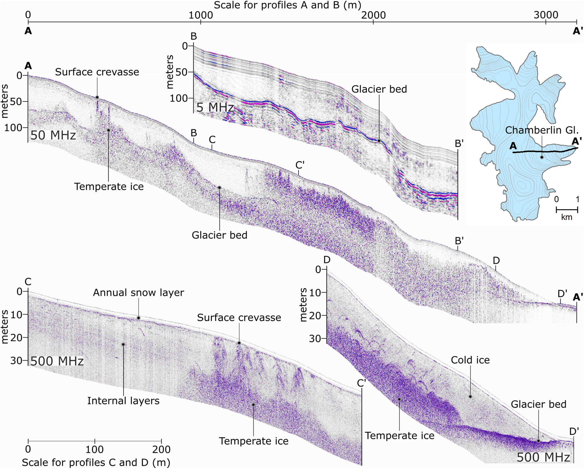
Figure 3. Examples of information on glacier geometry and ice characteristics observed in 500 MHz (not migrated), 50 MHz and 5 MHz (both migrated) GPR profiles. Profiles B, C and D are from various sections of profile A (insert map), which goes from the upper parts of the ice cap and down the centreline of the Chamberlin Gletsjer. The depth axes were determined using a velocity of 168 m μs−1 for ice.
Weak internal layering likely related to density or impurity contrasts within the ice is present in the upper regions of the Chamberlin Gletsjer (profile A in Fig. 3), however, no firn layer was observed along the profile, and the entire outlet glacier appears to be experiencing negative annual surface mass balance. A strong near-surface reflection in the high frequency dataset indicates the base of the annual snow layer (profile C and D in Fig. 3), which varies between close to 2 m near the plateau to ~1.5 m near the outlet glacier front. We observed few internal layers within the snowpack.
Further support to the notion of a link between crevasses and temperate ice comes from data collected on the largest western outlet glacier. Although ice thickness in this region generally exceeds that measured along Chamberlin Gletsjer (Fig. 3), a GPR profile collected from the front of the outlet glacier to the ice cap plateau (Fig. 4) shows transparent ice throughout and it is clear that the glacier, along this transect has neither crevasses or temperate ice.
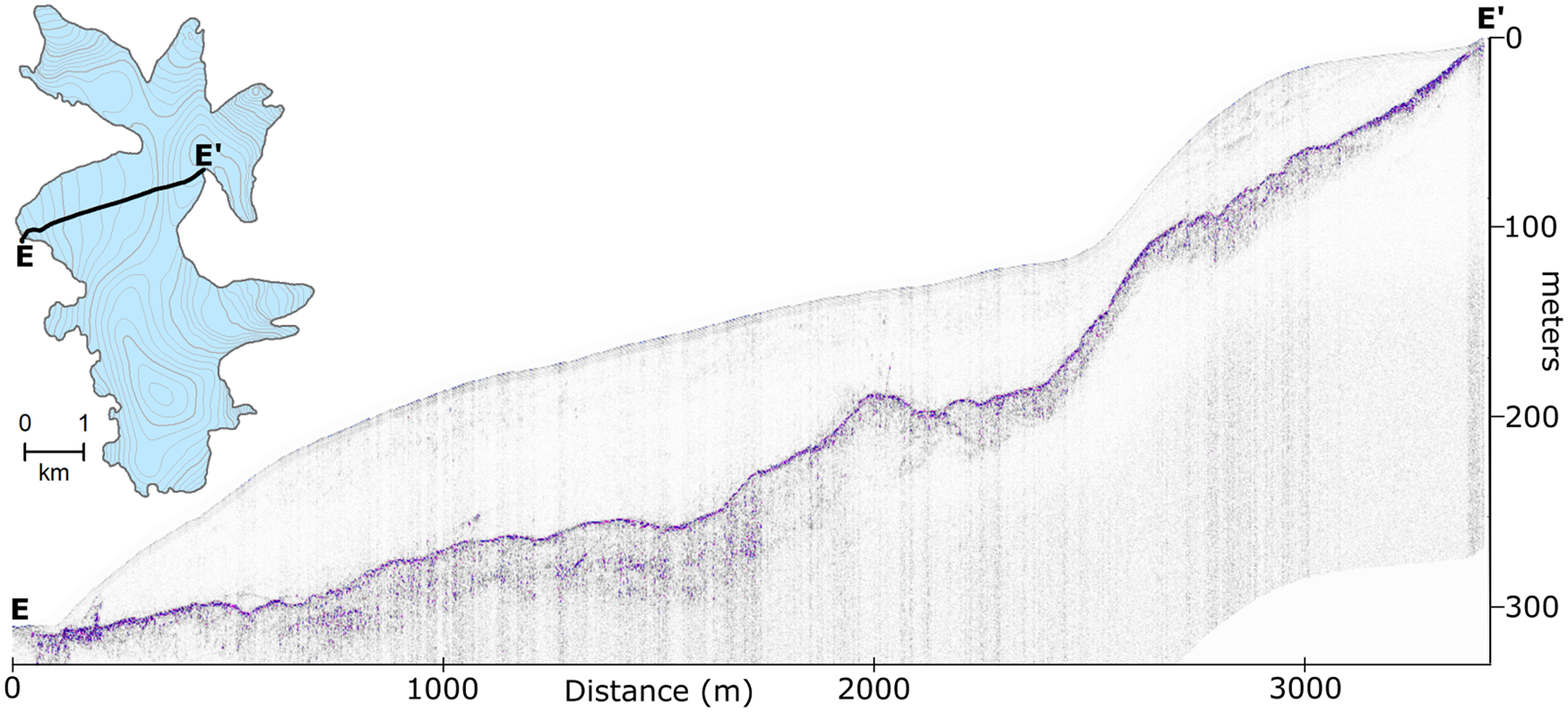
Figure 4. A 50 MHz radargram (profile E) collected from the front of the largest western outlet glacier and up across the upper plateau. Note the subglacial over-deepening (2000–2500 m distance from the terminus) downstream from the steep part of the glacier surface. The depth axis was determined using a velocity of 168 m μs−1 for ice.
Snow and firn distribution
The interpolation of snow and firn thickness must be used with caution due to the lack of measurements in large regions of the ice cap. It does however illustrate that there is little variation across the ice cap, with the snow depth generally ranging between 1.5 m and 2.0 m (Fig. 5). An underlying firn layer of less than 1 m thickness was observed in a few confined regions with north-western facing slopes (Fig. 5), coinciding with regions that are snow-covered in the late summer Sentinel-2B image (Fig. 1). However, no evidence of a deep firn layer was found in any of the GPR profiles, which suggests that most parts of the ice cap generally experience negative annual mass balance conditions. Measurements show that the snow is thickest in the catchment areas of the two largest southern outlet glaciers and thinnest in the flatter northern regions of the ice cap (Fig. 5). The only region that is adequately covered by snow thickness measurements is Chamberlin Gletsjer and the interpolation map clearly illustrates the decrease in snow thickness, which occurs towards the front of the outlet glacier. In all other regions, the snow and firn interpolation map (Fig. 5) relies on insufficient data and consequently the interpolated values are uncertain. Indeed, end-of-summer aerial images indicate the presence of a large accumulation area in the crevassed and consequently unsurveyed upper regions of the southern Chamberlin Gletsjer catchment.
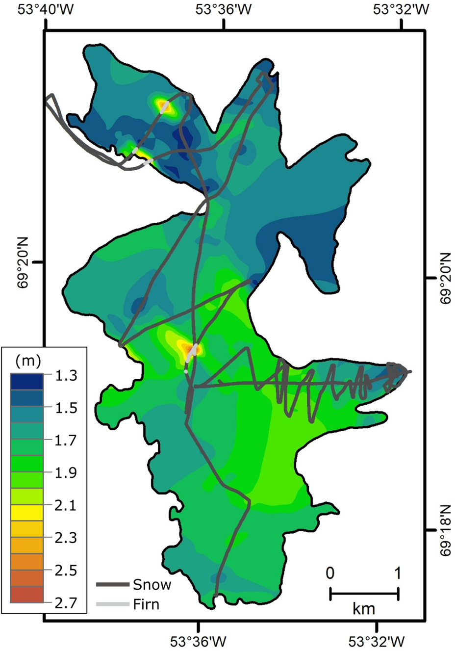
Figure 5. Interpolation of snow and firn thickness (0.1 m depth contours) together with the locations of 500 MHz GPR profiles where a snow layer (dark grey) and thin firn layer (light grey) were observed in the data.
Ice thickness, thermal regime and bed topography
Following processing and interpretation of the GPR dataset, we have obtained a consistent dataset of ice thickness observations that covers accessible regions of the ice cap (Fig. 6a). Results show that the thickest ice (maximum of close to 120 m ± 5 m) is found in the upper reaches of Chamberlin Gletsjer and the large western outlet glacier, while much thinner ice is found in the southern and northern parts of the upper ice cap plateau.
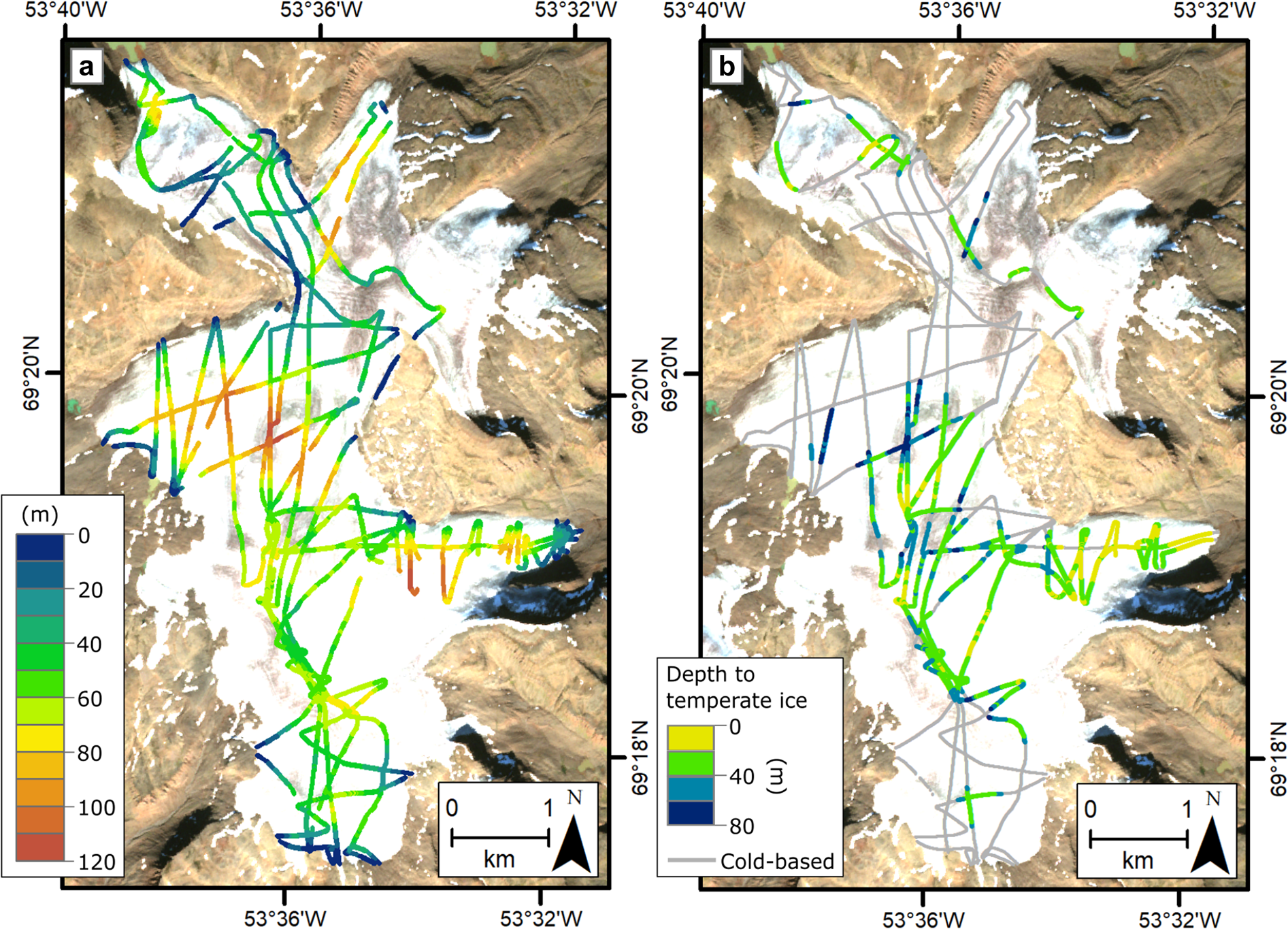
Figure 6. (a) Combined results of ice thickness measurements across Lyngmarksbræen Ice Cap. (b) Thermal regime, including depth to temperate ice in regions with polythermal conditions.
In terms of thermal conditions, Chamberlin Gletsjer and its catchment are polythermal, and the northern and southern parts of the ice cap are predominately cold throughout (Fig. 6b). Cold ice and snow overlay all temperate regions, but the depth to the temperate ice varies widely. In some regions shallow temperate ice is observed at 15–20 m depths, while in other regions the ice is predominantly cold but with patches of deep, relatively thin layers of temperate ice near the ice base (at ~60–80 m depth). Crevasses are observed in GPR data and satellite images along most profiles where temperate ice is present, and heavily crevassed regions correlate well with zones of near-surface temperate ice. In contrast, we find minor patches of deeper zones of temperate ice in crevasse-free regions of the ice cap and these observations appear unrelated to crevasses. The isolated patch of temperate ice observed at depth in the southern region of the large western outlet glacier represents one such example (Fig. 6b).
The interpolation map of ice thickness clearly illustrates the large variations in ice thickness which characterises Lyngmarksbræen Ice Cap (Fig. 7a). Using this map, we calculate the total 2017 volume of Lyngmarksbræen Ice Cap to be 0.82 ± 0.1 km3. When comparing the ice thickness interpolation map (Fig. 7a) with variations in surface (Fig. 1) and bed topography (Fig. 7b) we find that, in general, thin ice (<70 m) is located near ice divides in regions of high surface and bed elevations, while thicker ice is largely confined to lower elevations associated with the outlet glaciers. This is particularly true in the northern parts of the ice cap, where ice of only 25–30 m thickness separates the various outlet glacier catchments.
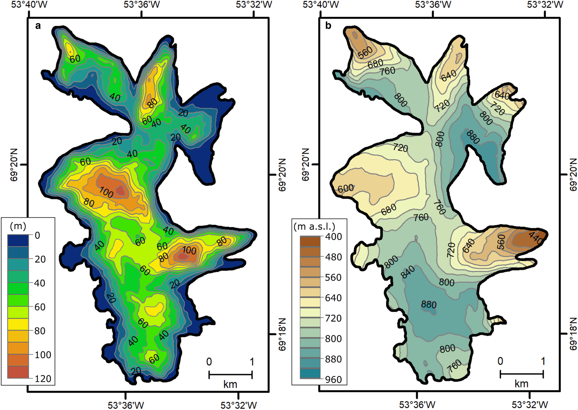
Figure 7. (a) Firn-corrected ice thickness (10 m colour contours) and (b) bed topography (40 m colour contours) at Lyngmarksbræen Ice Cap.
Despite a relatively flat surface topography on the upper ice cap plateau, the bed topography undulates and dips steeply towards the outlet glaciers that flow from the plateau in typical U-shaped valleys with subglacial over-deepenings (Fig. 4). The contrast between surface and bed slope is illustrated well by the GPR profile collected along the largest western outlet glacier (Fig. 4), which also shows an example of how ice thins considerably as it flows over high gradient bedrock. At the point of highest surface elevation (Fig. 1), the ice cap is about 70 m thick and covers a low gradient subglacial hill (Fig. 7b). The hill appears steepened towards Chamberlin Gletsjer as expected for a headwall of a valley or cirque glacier.
Discussion
Temperate ice formation and the potential for future dynamic change
In this paper we have mapped the extent of temperate ice on the Lyngmarksbræen Ice Cap from observed scattering in GPR measurements. The internal ice characteristics revealed by the GPR measurements along Chamberlin Gletsjer show patches of temperate ice beneath a thin (~15–20 m) cold surface layer, interspersed between zones of entirely cold ice. It is well established that zones of temperate ice will appear in GPR data as regions of strong scattering due to the presence of water-filled cavities (e.g. Travassos and Simões, Reference Travassos and Simões2004; Macheret and others, Reference Macheret2009; Wilson and others, Reference Wilson, Flowers and Mingo2013). Evidence of this comes from correlations between observed changes in borehole temperature and radar scattering (e.g. Wilson and others, Reference Wilson, Flowers and Mingo2013), suggesting that GPR measurements can be used as a proxy for direct borehole observations of glacier thermal regime. The multi-frequency approach presented here for Lyngmarksbræen Ice Cap prevents an underestimation of the extent of temperate ice, as have been documented in previous studies when the radar wavelength is large compared to the size (<1 m) of the water cavities (Smith and Evans, Reference Smith and Evans1972; Watts and England, Reference Watts and England1976; Jezek and Thompson, Reference Jezek and Thompson1982; Pettersson, Reference Pettersson2005). Uncertainty in the delineation of temperate ice from GPR measurements may occur in regions with many crevasses, where ringing of the radar waves can obscure the boundary to the temperate ice, possibly leading to an underestimation of the upper cold layer thickness. On Chamberlin Gletsjer, shallow temperate ice is observed both in crevassed regions where columns of diffractors extend from the glacier surface, as well as in nearby downstream regions without crevasses. Therefore, the scattering cannot be solely caused by disturbances as the emitted radar waves travel through the crevasses, and we are confident in the interpretation of temperate ice.
The large spatial variability in thermal ice conditions on Lyngmarksbræen Ice Cap requires some consideration. Temperature data from boreholes in the western GrIS ablation zone show that while the top ~10–15 m of ice is influenced by the cold air temperature, ice temperature below this depth reflects that of deeper ice flowing towards the glacier surface (Hills and others, Reference Hills2018). These findings correspond well with the shallow change from cold to temperate ice identified in some regions of Lyngmarksbræen Ice Cap, and the influence of surface temperature explains the lack of an entirely temperate ice column. Isolated diffraction hyperbolae observed within the cold layer and above the shallow temperate ice on Chamberlin Gletsjer could indicate a somewhat gradual transition from near surface cold conditions to temperate ice. The GPR measurements were collected before the onset of summer melting and the diffraction hyperbolae may originate from air- or water-filled voids that have persisted through the winter period. Water storing fractures have previously been documented in the upper ~15 m cold ice in regions without surface crevasses (Hills and others, Reference Hills2018), while diffractors observed at greater depth in GPR data collected on the outer cold regions of the western GrIS have been tentatively attributed to water inclusions originating from upstream crevassed regions (Brown and others, Reference Brown, Harper and Humphrey2017). Calculations have shown that water trapped in closed-off surface crevasses may persist in cold ice for years (Jarvis and Clarke, Reference Jarvis and Clarke1974), and it is not unlikely that similar processes could also explain the diffractors observed on Lyngmarksbræen Ice Cap.
The conditions observed at Chamberlin Gletsjer are not representative for all parts of Lyngmarksbræen Ice Cap, and although large zones of temperate ice do exist elsewhere, the remainder of the ice cap presents as largely cold-based. The nature of the observed temperate ice varies across the ice cap. Deep zones can be attributed to the combined effect of geothermal heat flux, a lower pressure melting point and increased strain heating near the base of thick ice; however, shallow temperate ice must be caused by other processes. Given the shallow snow and firn layer (1.5–2 m), active latent heat release from percolating meltwater in a deep firn layer cannot be the main factor in generating temperate ice within the surveyed regions of Lyngmarksbræen Ice Cap. Interpreted relic zones of temperate ice have been found both in the upper and thickest regions of Waldermarbreen in Svalbard (Karušs and others, Reference Karušs2022) and near the front of the small Kårsaglaciären in Sweden (Rippin and others, Reference Rippin, Carrivick and Williams2011). On both glaciers, the relic zones of shrinking temperate ice are thought to illustrate a lag in thermal change as the glaciers adjust from past periods of larger extent and a more developed firn layer (Rippin and others, Reference Rippin, Carrivick and Williams2011; Karušs and others, Reference Karušs2022). However, distinct differences exist between the characteristics of temperate ice at these two glaciers and that observed at Lyngmarksbræen Ice Cap, suggesting different origins. At Lyngmarksbræen Ice Cap, a strong spatial correlation exists between temperate ice and observations of surface crevasses, which suggests that the shallow zones of thick temperate ice are generated by active cryo-hydrologic warming as meltwater refreezing in crevasses release latent heat to the surroundings. While the importance of crevasse-driven cryo-hydrologic warming on ice temperature has been described in previous studies using various approaches (e.g. Jarvis and Clarke, Reference Jarvis and Clarke1974; Humphrey and others, Reference Humphrey, Harper and Pfeffer2012; Harrington and others, Reference Harrington, Humphrey and Harper2015; Lüthi and others, Reference Lüthi2015; Meierbachtol and others, Reference Meierbachtol, Harper, Johnson, Humphrey and Brinkerhoff2015; Poinar and others, Reference Poinar, Joughin, Lenaerts and Van Den Broeke2017; Hills and others, Reference Hills2018; Gilbert and others, Reference Gilbert2020; Seguinot and others, Reference Seguinot2020), the level of detail of the GPR measurements presented here provide new evidence of the complexity of temperate ice formations and the spatial variability which occurs as a result. It would require an unrealistic number of boreholes to resolve the variations in thermal conditions observed on Chamberlin Gletsjer, and the results offer further support to the notion that caution is required when relying on single borehole temperature measurements in regions where cryo-hydrologic warming may be significant (Lüthi and others, Reference Lüthi2015).
Thermal conditions at Lyngmarksbræen ice cap should also be considered in the context of possible temporal changes in temperate ice formation and extent, although a full discussion of all parameters affecting ice temperature in a changing climate is beyond the scope of this paper. During cold periods such as the Little Ice Age with increased ice thickness and less surface melting, temperate ice formation caused by strain heating near the ice base and the effect of ice thickness on the pressure melting point was likely proportionally more important at Lyngmarksbræen Ice Cap than it is today. In a warming climate, crevassed areas are expected to initially expand due to increased thinning, higher surface slope and enhanced ice velocity (Colgan and others, Reference Colgan2011, Reference Colgan2016). Excess surface melt draining through these conduits has the potential to further increase glacier velocity both through enhanced basal lubrication when water penetrates to the sole of the glacier, and by increased cryo-hydrologic warming of the ice (Phillips and others, Reference Phillips, Rajaram and Steffen2010, Reference Phillips, Rajaram, Colgan, Steffen and Abdalati2013; Colgan and others, Reference Colgan2011, Reference Colgan2016). Because of the strong present-day correlation between surface crevasses and thick temperate ice at Lyngmarksbræen Ice Cap, we hypothesise that the zones of temperate ice will grow in a warming climate and that ice velocity of the ice cap will increase as a result. The proposed thermal change from today's predominantly cold-based conditions to temperate ice would lead to a reduction in the timescale over which the glacier responds to changes in climate.
We still do not fully understand the temporal and spatial changes in ice dynamics associated with increased glacier meltwater in a warming climate, and the full extent of these positive feedback mechanisms are often not considered in studies of future glaciers dynamics (Lampkin and others, Reference Lampkin2018; Aschwanden and others, Reference Aschwanden2019). Recent years have seen extreme melting events occurring in Greenland, with the summer of 2019 being the lowest surface mass balance year on record (Tedesco and Fettweis, Reference Tedesco and Fettweis2020). Given the current observations on climate change and the probable influence of cryo-hydrologic warming feedback mechanisms on ice cap instability and dynamic mass loss, it is important that we further our understanding within this area of research to better include these processes into glacier flow models. The data presented here contribute towards this process by providing evidence to the importance of surface crevasses on cryo-hydrologic warming and of accounting for temporal changes in crevasses when modelling glacier behaviour in a changing climate.
Ice cap geometry and implications for future ice cap fragmentation
Like ice caps in general, Lyngmarksbræen Ice Cap is particularly sensitive to variations in climate, as even a small rise in the equilibrium line altitude (ELA) can lead to a major decrease in accumulation area when the ELA is situated near or at their flat upper regions (Oerlemans, Reference Oerlemans1997). In addition, due to the relatively low elevation of the coastal areas of Greenland and the significant changes observed in these regions (Hanna and others, Reference Hanna2013), GICs such as Lyngmarksbræen Ice Cap, are especially vulnerable in a warming climate. Modelling experiments conducted on other ice caps have shown that the nature of future change may vary widely depending on the distribution of ice (Giesen and Oerlemans, Reference Giesen and Oerlemans2010; Åkesson and others, Reference Åkesson, Nisancioglu, Giesen and Morlighem2017; Zekollari and others, Reference Zekollari, Huybrechts, Noël, van de Berg and van den Broeke2017). Some ice caps, like Lyngmarksbræen Ice Cap, have a rough bedrock topography where peaks and ridges covered in relatively thin ice influence the interior ice divides, and thick outlet glaciers flow in deep valleys and troughs (e.g. Macheret and others, Reference Macheret2009; Boon and others, Reference Boon, Burgess, Koerner and Sharp2010; Åkesson and others, Reference Åkesson, Nisancioglu, Giesen and Morlighem2017). Other ice caps are located on relatively flat plateaus and have the thickest ice in the interior regions near surface domes (e.g. Dowdeswell and Evans, Reference Dowdeswell and Evans2004).
The results of the ice thickness distribution and revealed bed topography at Lyngmarksbræen Ice Cap indicate that ice may likely disappear in the higher elevation regions at an early stage of glacier retreat, effectively fragmenting the ice cap into individual retreating valley glaciers and cirques. Several important mechanisms will influence the rate of glacier retreat and ice cap fragmentation at Lyngmarksbræen Ice Cap. Studies have found that as an ice surface lowers and steepens in a warming climate due to differential changes in surface mass balance (Zekollari and others, Reference Zekollari, Huybrechts, Noël, van de Berg and van den Broeke2017), feedback processes such as increased shading and wind driven snow accumulation in developed hollows may act to delay recession of outlet glaciers that are sheltered by valley walls (Braun and others, Reference Braun, Hardy and Bradley2004; Boston and Lukas, Reference Boston and Lukas2019). Also, once ice cap disintegration begins, newly exposed bedrock will increase the melting of nearby ice further due to positive feedback mechanisms from the albedo change (Paul and others, Reference Paul, Kääb, Maisch, Kellenberger and Haeberli2004; Jiskoot and others, Reference Jiskoot, Curran, Tessler and Shenton2009).
Disequilibrium of the world's ice caps have been documented in detail for ice caps in Iceland (e.g. Björnsson and Pálsson, Reference Björnsson and Pálsson2020), Norway (e.g. Åkesson and others, Reference Åkesson, Nisancioglu, Giesen and Morlighem2017) and northern Greenland (e.g. Sugiyama and others, Reference Sugiyama2014; Zekollari and others, Reference Zekollari, Huybrechts, Noël, van de Berg and van den Broeke2017), but similar trends are observed worldwide (Fox-Kemper and others, Reference Fox-Kemper2021). Observations at Lyngmarksbræen Ice Cap show that this ice cap is also experiencing significant mass loss resulting in a reduced accumulation area, absence of a firn layer in most regions, and glacier retreat (Yde and Knudsen, Reference Yde and Knudsen2007). This is consistent with surface mass balance observations produced since 2016 at Chamberlin Gletsjer by the GlacioBasis Disko monitoring programme (Citterio, Reference Citterio2021). The disequilibrium of Lyngmarksbræen Ice Cap with today's climate suggests that future glacier retreat will be substantial. Although somewhat speculative until a thorough modelling study has been conducted on Lyngmarksbræen Ice Cap, we hypothesise that the observed ice cap geometry shows that the ice cap has previously divided into smaller ice bodies located where large outlet glaciers and the thickest ice are currently found, and that this process will also likely occur in future. This fragmentation will likely begin within the coming decades in the central northern region, where ice thickness in 2017 was less than 30 m over the highest elevated subglacial bedrock.
Conclusions
In this study we present multi-frequency GPR data collected at Lyngmarksbræen Ice Cap in Greenland in 2017. From this dataset, we have constructed the first map of ice thickness of the ice cap and provided new information on surface mass balance and thermal conditions. The GPR survey shows a maximum ice thickness of ~120 ± 5 m and a total ice volume of 0.82 ± 0.1 km3. Less than 30 m thick ice separate outlet glacier catchments in the northern parts and measurements of snow and firn illustrate that the ice cap is experiencing a negative surface mass balance in most regions. In addition to information on snow and ice thickness, GPR images show highly variable cold and temperate ice conditions, which we interpret as primarily caused by cryo-hydrologic warming from percolating and refreezing meltwater in crevasses. Cryo-hydrologic warming has the potential to cause large-scale instabilities and dynamic mass loss, and temporal changes in thermal regime and its effects on ice dynamics during ice thinning and recession should be given careful consideration when designing glacier modelling experiments.
From the new observations of the bedrock topography and the distribution of ice, we suggest that in a warming climate, Lyngmarksbræen Ice Cap will separate into individual valley glaciers and cirques surrounded by higher elevated ice-free bedrock. It is expected that a fragmentation of the ice cap into smaller units will occur in the immediate future, which will have a societal impact on the Qeqertarsuaq community relying on the glacier for economically important tourist activities.
Acknowledgements
We would like to thank editor Shad O'Neel and reviewers Elizabeth Case and Peter Jansson for their insightful comments and suggestions for improvements to the original draft of the manuscript. The study was funded by an INTERACT Transnational Access grant (project ICELYN). We thank Kjeld Akaaraq Mølgaard and Gitte Henriksen for logistic support in relation to our stay at Arctic Station. Access to the ArcticDEM was provided by the Polar Geospatial Center under NSF-OPP awards 1043681, 1559691 and 1542736. GlacioBasis Disko is funded by the Danish Energy Agency as a component GEM (Greenland Ecosystem Monitoring).
All data presented in this paper are available upon request to author Mette K. Gillespie (mette.kusk.gillespie@hvl.no).


 Open access