


Introduction
One important aspect of the ongoing global-change debate is the response of the East Antarctic ice budget to climatic changes. This paper presents field observations and results of radar surveys of the sub-ice topography of selected areas in Victoria Land and north Victoria Land, Antarctica, from which evidence for fluctuations of the ice level and different glacial regimes in the recent and more distant past will be derived. The probable causes of the observed changes will be identified on the basis of the results from numerical models investigating the response of large ice caps to climatic changes. For this purpose, an idealized model configuration — a flat-based, initially ice-free continent with a radius of 1750 km — was chosen. The numerical simulations with this model continent include the following stages:
Development of an ice cap to full size on an initially ice-free continent, assuming a warmer climate than today (“Tertiary climate”).
Transition of the ice cap to a new configuration following a change from a “Tertiary” to a cold-stage climate.
Transition from a glacial stage to an interglacial stage climate.
All field surveys were carried out on and in the vicinity of various blue-ice fields, of which two are known for their high meteorite concentrations. The field work was done during the following expeditions:
The GANOVEX IV expedition (1984–85) by the Bundesanstalt für Geowissenschaften und Rohstoffe (BGR) to north Victoria Land, an expedition to the Allan Hills area in 1988–89’ (logistically supported jointly by the U.S. National Science Foundation (U.S. NSF, U.S.A.), Max-Planck-Institut, Mainz, Germany, and BGR, Germany), the Italian expedition (1990–91) to north Victoria Land, the GANOVEX VI expedition (1990–91) by BGR to Victoria Land.
Previous Work
A vast amount of literature on the glacial geology in the coastal areas of the East Antarctic continent has been summarized in Reference Denton and HughesDenton and Hughes (1981). A summary of aspects of the late Wisconsin and early Holocene glacial history of the Ross Embayment can be found in Reference Denton, Bockheim, Wilson, Stuiver and BindschadlerDenton and others (1991).
Glacial geologists have long suspected the East Antarctic continent of having been at least periodically covered in the past by more massive ice sheets. The evidence for this is the glacial striations on top of nunataks near the Polar Plateau, which rise up to 1000 m above the current ice level (see e.g. Reference Denton, Prentice, Kellogg and KelloggDenton and others, 1984; Reference Höfle and MeerHöfle, 1987; Reference Höfle, Delisle, Herpers, Bremer,, Hofmann and WölfliHöfle and others, 1992). However, episodic rapid uplift during the Pliocene and/or Pleistocene (see e.g. Reference Behrendt and CooperBehrendt and Cooper, 1991) might offer an alternative interpretation. Additional evidence for temporarily thicker ice sheets comes from marine geologists, who have identified a number of major advances of Antarctic ice on to the Antarctic continental shelf (see e.g. Reference Hinz and BlockHinz and Block, 1983; Reference Hinz and KristoffersenHinz and Kristoffersen, 1987; Reference Bartek, Vail, Anderson, Emmet and WuBartek and others, 1991). Such events must be accompanied by a greater ice thickness in more central parts of Antarctica.
The discovery of glacially transported diatoms of late Pliocene age 2.2 km above sea level in the Transantarctic Mountains (Reference HarwoodHarwood, 1983, Reference Harwood, Thomson, Crame and Thomson1991) has been interpreted as evidence of periodically large-scale retreats and readvances of the ice sheet, during which the Wilkes Basin at least once became ice-free and was invaded by sea water. 10Be dating of rock exposures from various nunataks in north Victoria Land indicates a regionally 1000 m higher ice stand sometime 2.7–4.0 Ma B.P. (Reference BremerBremer and others, 1991). One is tempted to interpret these results as evidence of massive fluctuations of the East Antarctic ice sheet during the warmer Tertiary climate in comparison to the current interglacial stage. Substantial changes in sea level would result from such a scenario. Limited evidence to this effect is available from work of marine geophysicists (see e.g. Reference Haq, Hardenbol and VailHaq and others, 1987).
Little evidence for drastic changes in ice thickness on the Polar Plateau is available for the period of the latest glacial/interglacial cycles. Reference Denton, Bockheim, Wilson, Stuiver and BindschadlerDenton and others (1991) argued that the last advance of the Ross Ice Shelf during the Wisconsin was accompanied by little elevation change on the Plateau.
Various workers have attempted to simulate numerically the response of the Antarctic ice sheet to variations of sea level, climate and other parameters (see e.g. Reference OerlemansOerlemans, 1982; Reference Budd, Jenssen and SmithBudd and others, 1984; Reference HerterichHerterich, 1988; Reference Huybrechts and OerlemansHuybrechts and Oerlemans, 1988). These models have demonstrated the major influence of the following two phenomena on ice-sheet growth or decay:
Sea-level fluctuations caused by glaciation/deglaciation in the Northern Hemisphere (Reference Peltier and TushinghamPeltier and Tushingham, 1991) or other tectonic processes affect directly the behaviour of ice shelves and ice sheets. A drop in sea level allows ice shelves and ice sheets to advance further out on to continental shelf areas than at times of rising sea level.
The change of snow accumulation due to a climate change has an immediate effect on the thickness of ice sheets. As will be shown again below, the increased snow accumulation caused by the climatic warming since the last glacial stage has locally changed the ice thickness by several hundred metres.
Previously published models have concentrated either on the overall behaviour of the Antarctic ice sheet or on the ice shelves. The model presented below concentrates on the question of the specific reaction of the Antarctic ice sheet in near-coastal areas, that is, in places where meteorite traps are known to have existed for the past several hundred thousand years. A detailed discussion of all Antarctic meteorite collection sites has been given by Reference Cassidy, Harvey, Schutt, Delisle and YanaiCassidy and others (1992).
The Model
The intensity of glaciation of a continent reacting to climate changes is calculated in two dimensions. The response of the model ice sheet is driven by essentially three key factors:
Creep law for ice (Reference NyeNye, 1959).
An accumulation function related to climate as shown in Figure 1a (more details in Reference DelisleDelisle (1991)).
Past climate scenarios as derived from various studies on isotopes in Antarctic ice cores and deep-sea sediments (see e.g. Reference Miller, Fairbanks and MountainMiller and others, 1987; Reference Lorius, Barkov, Jouzel, Korotkevich, Kotlyakov and RaynaudLorius and others, 1988).

Fig. 1. Snow accumulation vs mean annual temperature used in the numerical model. Open circles give values measured at Antarctic stations (top). The mean annual air-temperature distribution (model I) is assumed over an initially ice-free continent at t = 0 (bottom).
The model calculates in iterative fashion ice flow and the temperature field in the ice body and the underlying bedrock. The set of equations used to calculate the growth of an ice sheet as a function of pre-defined climate changes has been given in Reference DelisleDelisle (1991). To this has been added the effects of frictional heat in ice (from Reference Budd, Young and RobinBudd and Young, 1983) and a terrestrial heat-flow component of 60 mW m−2 at the ice base at t = 0.
The model assumes, at t = 0, an ice-free circular continent with a radius of 1750 km. A mean annual temperature and an adiabatic gradient in air as shown in Figure lb is superimposed on its surface. The growing ice sheet will pass through a time period equivalent to climatic conditions, which we assume to have existed during the late Tertiary (warmer climate than today), followed by a Quaternary climate cycle (glacial and interglacial stage). The sequence of idealized climate changes as a function of time is shown in Figure 2. The air temperatures above the model ice sheet were adjusted accordingly during each climate change. The length of time for the idealized “Tertiary” and “Quaternary” periods was chosen to be sufficiently long to ensure that ice sheets C and A run into steady-state configurations. Four different models will be presented starting at t = 0 with different initial conditions as summarized in Table 1. All models will end up with an ice-sheet configuration comparable to conditions observed in East Antarctica today.

Fig. 2. Assumed variation of mean annual temperatures. Shown is a fictitious course of climate change. Calculated ice sheets respond to the assumed climatic changes by taking up the new air temperatures on their surfaces and through the changing accumulation rates (see Fig. 1).
Table 1. Table 1

The calculated changes of the ice profiles in response to the climatic settings as defined by A and Β in Figure 2 are shown in Figure 3A–C. The results obtained for A, Β and C are discussed below separately.

Fig. 3. Calculated ice-sheet profiles for a glacial stage (A), interglacial stage (B) and a “late Tertiary” climate (C).
Climatic Setting A
Case A gives ice-sheet configurations at the end of a prolonged cold period (glacial stage). The four models predict a range of 3.8–2 km in ice thickness at the centre point of the ice sheets. The ice-sheet configuration in peripheral areas is practically the same for all models considered. The low precipitation values during a glacial stage cause the ice cap to reduce its overall thickness, except along the periphery, in comparison with its configuration in warmer climates. The flanks steepen in response to the decreased plasticity of the ice and lower flow velocities.
Climatic Setting Β
Case Β gives ice-sheet configurations 10000 years after the beginning of an interglacial stage (equivalent to current climate) immediately following case A. Within this period, the model ice cap has adapted to a large extent to the climatic warming in all four cases.
The calculations predict, in agreement with numerous models of other workers, for the transition from a glacial to an interglacial stage a moderate increase in ice thickness in central parts of the ice cap as a consequence of increased snow accumulation, and decreasing ice thickness in peripheral areas of the ice sheet. The difference between the ice-sheet configurations Β and A for the four model cases considered is shown in Figure 4. The ice-thickness reduction in peripheral areas is due to two factors:
The increase in snow accumulation at the beginning of the interglacial stage rapidly displaces the cold ice at the front of the ice sheet.
Increasing ice temperatures cause increased rates of ice deformation, which translates into increased ice velocities. The cold ice of the ice front, where the overall highest ice velocities occur, is therefore rapidly replaced.

Fig. 4. Calculated differences in ice thickness between an interglacial and glacial stage. The ice thickness grows in the central part of the ice sheet and shrinks in near-coastal areas during an interglacial stage.
The overall effect, according to our model, translates into regional thinning of the ice in the peripheral areas.
Climatic Setting C
Figure 3c gives the ice-sheet configurations for a climate 8 °C warmer than the present as it might have existed periodically during the late Tertiary (see e.g. Reference Miller, Fairbanks and MountainMiller and others, 1987). The overall increased snow accumulation translates in all model cases into maximum ice-thickness values ranging between 4.2 and 4.5 km at the innermost point of the ice sheet. However, the surface slope at the periphery is much less than for case Β (current climate). The difference between the ice-sheet profiles C and Β is given in Figure 5. The calculated profiles for C have developed essentially within 30000–40000 years after initiation of the ice sheet on an initially ice-free continent.

Fig. 5. Calculated differences in ice thickness between “interglacial stage” and “late Tertiary” ice sheets. The ice thickness grows in the central part of the ice sheet and substantially shrinks in near-coastal areas in a climate 8 °C warmer than today.
The profiles represent the quasi-stationary ice-sheet configurations for the given climatic conditions, if one does not introduce appropriate equations to allow surging of the ice sheet.
For comparison, Figure 6 shows horizontal ice-velocity components on the ice-sheet surface for cases A, Β and C at the zones where wet conditions at the base of the ice sheet are predicted by the model calculations (here the case of model III is shown). A “late Tertiary” ice sheet (C) differs from an “interglacial — or a glacial stage” ice sheet in two respects. A “late Tertiary” ice sheet
is wet-based in peripheral zones (roughly, the outer 600 km of the ice sheet). Such conditions occur under “interglacial/glacial stage” ice sheets only within a radius of 500–600 km from the centre point. The rate of transport of cold ice to basal regions is in the latter case insufficient to counteract basal melting induced by terrestrial heat flow, in particular, when the ice sheet has developed fully.
has ice velocities at the surface in excess of 100 m a−1 within about 300 km from the ice front, which in reality should lead to periodic surge events. Comparable ice velocities are reached by an “interglacial stage” ice sheet only at an ice tongue and not at all by a “glacial stage” ice sheet.

Fig. 6. Horizontal ice velocities at the ice-sheet surface (model III) in various climatic settings. Note the shift of the wet-based basal zone from the periphery to the centre as the climate deteriorates.
Figure 7 shows the temperature distributions based on model III 500 and 1700 km from the centre point of the ice sheets for cases A, Β and C. The coldest ice sheet (A) shows the least deformation of the temperature-depth profile by convective and advective ice transport. An almost linear increase of ice temperatures near the bottom is predicted except in near-coastal regions in case C. The high amount of ice melting caused by high internal frictional forces near the ice base raises, in the latter case, the near-basal ice temperature to the melting point.

Fig. 7. Temperature-depth distribution for climates A-C 500 and 1700 km outbound from the centre point of the ice sheet (model III).
Field Observations
Field observations indicating past ice fluctuations within and at the western boundary of the Transantarctic Mountains are presented below. The localities of the sites visited are shown in Figure 8.

Fig. 8. Location of surveyed blue icefields in Victoria Land and north Victoria Land. Regions 2000 m above m.s.l. are shaded. FRO = Frontier Mountain; MJ = Mount Joyce; BP = Brimstone Peak; GN = Griffin Nunatak; ALH = Allan Hills.
Allan Hills Icefield
The surface and sub-ice topography, as well as the dynamics of the ice flow across the region to the west of Allan Hills, Victoria Land, have already been described in Reference Delisle and SieversDelisle and Sievers (1991) and Reference Schultz, Annexstad and DelisleSchultz and others (1990). Figure 9 shows a cross-section from Allan Hills westwards along the existing triangulation network (Reference Annexstad, Schultz, Oliver, James and JagoAnnexstad and Schultz, 1983). The westward-sloping blue icefield adjacent to Allan Hills flows at several cm a−1 northwestwards, while being exposed to a sublimation rate of about 5 cm a−1 (see Reference DelisleDelisle and others, 1989). This icefield, currently not resupplied by advected ice, decays at this time and will, assuming an unchanged sublimation rate, have disappeared in about 5000 years. This blue icefield has obviously been formed in a recent period of a regionally higher ice stand with ice flow toward Allan Hills from the west. The above numerical model suggests that a higher ice stand most likely existed for the last time during the termination of the last glacial stage. This situation is the more intriguing as Allan Hills Icefield is distinguished by one of the major Antarctic meteorite concentrations. The increase in ice thickness cannot have exceeded the height of Allan Hills. Otherwise, ice flow would have transported away the currently exposed blue ice with entrapped meteorites with terrestrial ages of typically several hundred thousand years (Reference Nishiizumi, Elmore and KubikNishiizumi and others, 1989).

Fig. 9. Ice-surface and sub-ice topography along a profile from Allan Hills westwards. The blue icefield next to Allan Hills slopes and flows westwards and has no nearby source area. The ice was deposited during an apparently recent period with a higher ice stand.
Griffin Nunatak — Brimstone Peak
Surface slopes and the ice-thickness distribution of the icefield around these two nunataks were investigated in detail in 1991. On the leeside of both mountains, large blue icefields exist, on which ample evidence of a recently higher ice stand has been observed. Technical details on the radar instrumentation used to determine the sub-ice topography can be found in Reference Delisle and SieversDelisle and Sievers (1991).
Griffin Nunatak
The blue icefield to the northeast of Griffin Nunatak is on average 825 m thick as measured by radar (Figs 10 and 11) and rests on an almost flat bottom. The surface slope across this icefield is on average 7 m km−1, which implies very slow ice flow. The ice near the northeast flanks of Griffin Nunatak is covered by a continuous layer of debris, protecting the underlying ice from the heat radiation from adjacent rock walls. Therefore, only few ice depressions (bergschrund) along the flanks of Griffin Nunatak have developed. Four moraine trains, which were formed as lateral moraines during the last ice advance over Griffin Nunatak, run across the blue icefield (Fig. 10). Two of the lateral moraines delineate today exactly the extension of the valleys, through which ice streams over-riding Griffin Nunatak would have had to flow. Horizontal flow of blue ice since that event was obviously insufficient to deform the orientation of these moraines. Many rock fragments lie across the blue-ice surface between the moraine trains, which probably were transported at the base of the former over-riding ice stream. All these observations point to a regionally higher ice stand in the last few thousand years.

Fig. 10. Surface topography of the Griffin Nunatak and Brimstone Peak area. Located to the north of the northeast corner of Brimstone Peak is an inactive crevasse field (black area; see discussion in text) and two moraines (dotted area) resting on about 600 m of blue ice.
The trend of the last over-riding event is almost perpendicular to the deep glacial valley that separates Griffin Nunatak from Brimstone Peak. In the distant past, a drastically different glaciological flow regime, oriented west-east, must have existed in the region.
Brimstone Peak
The surface and sub-ice topography of the blue ice to the east and north of Brimstone Peak are very complex (Figs 10 and 11). Near the flanks of Brimstone Peak, in particular at the north face, deep depressions in the ice surface and subsequent formation of meltwater lakes have developed. To the northeast of Brimstone Peak at distances > 2 km, large areas of blue ice are covered with a thin rock veneer consisting of fist-size or larger fragments, which might be the remnants of a basal moraine of a former over-riding ice stream. About 2 km north of the northeast corner of Brimstone Peak, two moraines (shown in Figure 10 near the 1600 m contour), consisting on the southern end primarily of Beacon Sandstone with large inclusions of fossil wood and, on the northern end predominantly of Ferrar dolerite, are perched on top of 600 m of blue ice. A number of shear planes indicate shortening of the moraines along the long axis. The moraines rest in part on, and in part next to, a steep ice slope. The details of origin, path and extent of the previous over-riding ice stream that deposited the moraines are unclear.
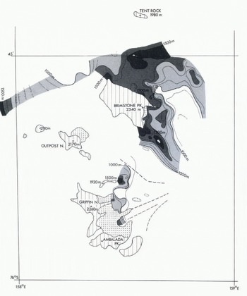
Fig. 11. Sub-ice topography of the Griffin Nunatak and Brimstone Peak area.
The first outcrop to the north of Brimstone Peak, about 4 m above the current ice level, shows glacial striations indicating previous glacial flow from the west-northwest. These striations incised in soft Beacon Sandstone presumably originated from the last episodic higher ice stand.
Large boulders of ice-transported Beacon Sandstone of fresh appearance rest about 300 m above the current level on the northern flank of Brimstone Peak, which itself is composed exclusively of a succession of basaltic flows of Jurassic age (the fine-grained equivalent to the Ferrar dolerite). Ice-cored scree slopes rise about 200m high along the east face of Brimstone Peak. Both observations are again indicative of a higher ice level in the recent past.
The most unusual feature on this blue icefield is a system of metre-wide crevasses (1 km to the north of the northeast corner of Brimstone Peak; see also Figure 10), which cannot be explained by current ice-flow processes. Close inspection revealed that no fresh cracks in the ice exist. All openings show signs of melting at the lateral walls. The bottoms of all cracks are closed by frozen meltwater. This feature is probably the remnant of a former crevasse system active at a time of a recently higher ice stand.
A refrozen meltwater lake, located at the eastern end of the northern face of Brimstone Peak, is easily distinguished from the surrounding glacier ice by its deep blue color and the high amount of frozen-in gas bubbles with diameters of up to 1 cm. A 2 m wide deep blue fresh-water ice band runs from the north through a blue icefield downslope toward the refrozen lake, apparently the remnant of a former meltwater stream. The blue meltwater lake ice is highly deformed as it has been squeezed by the surrounding glacier ice against the mountain face and now shows substantial relief (Fig. 12). The lake now forms the deepest point of the regional icefield. It appears that this area was exposed to a warmer climate for a limited time period after the last glacial stage, which might be equivalent to a suspected hypsithermal event 4—7 ka ago, for which evidence based on the characteristics of Holocene sedimentation on the Antarctic continental shelf was reported by Reference Domack, Jull and NakaoDomack and others (1991).
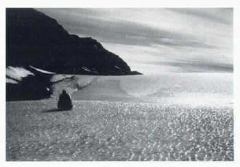
Fig. 12. A refrozen meltwater lake (dark surface) is pushed by glacier ice (lighter surface) against the mountain. Note the substantial relief of the refrozen lake.
Mount Joyce
The ice surface to the east of Mount Joyce slopes northeastwards toward the Ross Sea. An ice divide has developed between Burrage Dome and the northern tip of Mount Joyce (Fig. 13). Ice to the west of Mount Joyce flows northwards. Two moraine trains lie on blue ice to the northwest and west of the northern tip of Mount Joyce. They developed as lateral moraines during an earlier period of generally greater ice thickness and glacial flow towards the north-northwest toward the upper part of Drygalski Ice Tongue. Once again, these moraines seem to have suffered little displacement by the reorientation of ice flow towards the north-northeast after the end of the latest higher ice stand. This is again interpreted as evidence for their somewhat recent origin.

Fig. 13. Surface topography of the Mount Joyce area. Dashed lines (north of Mount Joyce) show prominent moraine trains deposited presumably during the last glacial stage.
Burrage Dome to the north of Mount Joyce is covered with many erratics (predominantly Ordovician granites as exposed to the east at and around Mount Stephen). Northwest-southeast oriented glacial striae are ubiquitously present at the southern tip of Burrage Dome, again evidence for an episode of a regionally northwestwardly directed flow.
The sub-ice topography of this area (Fig. 14) is unrelated to that episode. The time-dominated ice movement is directed towards the northeast. Deep glacial valleys have been formed in the past. The characteristics of the radar reflections obtained in this area imply that the ice is currently frozen to its bed.

Fig. 14. Sub-ice topography of the Mount Joyce area.
Frontier Mountain
Frontier Mountain acts as an obstacle to ice flowing from the Polar Plateau toward the catchment area of Rennick Glacier. Large blue icefields have developed to the northeast on the lee side of Frontier Mountain as well as of other nunataks in the vicinity. The mass loss, by sublimation, of ice from the blue icefield to the northeast of Frontier Mountain causes the regional ice stream to divert some of its mass toward the lee side of Frontier Mountain (Fig. 15). Wherever mountain valleys open to the northeast, deep depressions in the icefields were formed under the influence of enhanced radiation from the valley walls and high sublimation rates due to the action of foehn winds across the mountain.

Fig. 15. Regional ice flow around Frontier Mountain. “Meteorite Valley” is located near the southeast end of the mountain.
One valley at the southeast end of Frontier Mountain (Fig. 15) is known for its high meteorite concentration on blue ice (Reference DelisleDelisle and others, 1989). It is unofficially called “Meteorite Valley”.
The valley entrance is crossed by an ice ridge (Fig. 16c). Boulders with diameters of up to 3 m rest on the ridge top and most meteorites were found there. The valley 5 km to the northwest shows the exact opposite situation. The ice surface at the valley entrance forms a depression, which is delineated by a band of large boulders (Fig. 16a).

Fig. 16. The current field situation in “Meteorite Valley” (c) can best be explained by an inversion of topography induced by ice-level fluctuations due to the glacial/interglacial cycle. Glacial period = (a), transitional period = (b) and current interglacial stage = (c). Meteorites are found in the boulder region on the ice ridge over the moraine.
The development of the surface topography in “Meteorite Valley” can be explained by an inversion of topography as depicted in Figure 16a–c. In the initial stage, a higher ice level prevailed. Local valley-glacier ice and blue ice from outside the valley (Fig. 16a) met at the valley entrance, where horizontal ice flow from both sides approached zero. Sublimation caused a shallow depression in the zone of slow ice flow, in which ice-transported rock material, primarily rocks and boulders from the surrounding rock walls and from the glacier beds, and meteorites entrapped in ice, gathered with time. The regional ice level was lowered, as the climate warmed up. A meltwater lake formed in the depression. The rock material and the meteorites became immersed (Fig. 16b) in water. Evidence to this effect is available through the exceptionally high uranium content of all meteorites from “Meteorite Valley”. The concentration can be explained by prolonged leaching of uranium from local granitic rocks by meltwater and diffusion into the meteorites (for more details see Reference DelisleDelisle and others (1989)). In the case of “Meteorite Valley”, the meltwater lake has now receded far to the rear of the valley, while the former ice depression forms a topographic high, not nourished by ice flow from either side and protected against sublimation by the rock veneer on its surface (Fig. 16c).
Ice from the Polar Plateau forms a snow-and-ice cliff overlooking Frontier Mountain at the rear end of “Meteorite Valley” by about 50 m (see Figure 3 in Reference DelisleDelisle and others (1989)). However, the ice is apparently too cold to flow into the valley. A more than modest increase in ice thickness would cause the ice from the Polar Plateau to make its way through the valley northwards, thereby destroying the existing meteorite concentration.
Discussion
The four models presented on ice-sheet development under variable climatic conditions have produced compatible results, which are believed to indicate the trend and order of magnitude of changes that one might expect for an Antarctic ice sheet in response to climatic fluctuations since the late Tertiary. The available field evidence supports the numerical results as will be shown below.
The numerical model suggests a drastically different behaviour of the East Antarctic ice sheet during warmer climates of the late Tertiary. The ice thickness in the centre of East Antarctica should have surpassed the current values by several hundred metres. In near-coastal regions, in particular at sites also known for their meteorite occurrences today, 300–400 m thinner ice is predicted. The peripheral areas of the ice sheet were perennially warm-based and should have caused much more erosion at the bedrock than the present ice regime. Given the then existing wet-based conditions over large areas and the very high flow velocities, small-scale maybe even intermittently large-scale, surge events cannot be precluded.
Radar surveys across the Allan Hills and Griffin Nunatak Icefields clearly indicate a once drastically different ice-flow regime. Deeply eroding ice flow towards east to southeast was once predominant in the Griffin Nunatak area (Fig. 11). The sub-ice topography at Allan Hills and near Western Icefield was formed in part by local, alpine-type glaciers that flowed to the southwest-northwest towards the continent (figures 4 and 5 in Reference Delisle and SieversDelisle and Sievers (1991)) This is compatible with the view of Reference Webb, Thomson, Crame and ThomsonWebb (1991), Reference Harwood, Thomson, Crame and ThomsonHarwood (1991) and Reference McKelvey, Webb, Harwood, Mabin, Thomson, Crame and ThomsonMcKelvey and others (1991) of intermittent ice-free basins to the west of the Transantarctic Mountains during the early and late Pliocene, into which these glaciers could have drained. A more conservative view would be to assume a several hundred meters on average lower ice level during warmer Tertiary climates, as predicted by the above model.
Reference Nishiizumi, Kohl, Arnold, Klein, Fink and MiddletonNishiizumi and others (1991) have measured the exposure and erosion history of the Allan Hills region on the basis of the cosmic-ray-produced 10Be and 26A1 content in the surface rocks. 10Be with a half-life of 1.5 × 10⁶a and 26Al (t ½ = 0.705 × 10⁶a), have different cosmic-ray-induced production rates and offer independent measurements on the time of the surface exposure. The data by Nishiizumi and others suggest that “the Allan Hills have been exposed above the present ice surface for more than half a million years and that the erosion rate for these rocks is less than a few times 10−5 cm a−1.” The oldest “minimum-exposure age” measured on a sample from an outcrop 15 m above the current ice level was 1.4 (±0.34) × 106 years. They found that the slightly different exposure ages obtained from the concentrations of the two isotopes suggest only intermittent and short-term burial of the rock surfaces by snow or ice since their first exposure. These results indicate either higher erosion rates during the early Pleistocene, producing fresh rock surfaces at a faster rate than today or, alternatively, require a persistent glacial cover of the area before the mid-Pleistocene. A glaciated terrain is required at least at some stage as a source area for the above-mentioned alpine type, westward-moving glaciers.
The above scenario does not preclude the possibility of major advances of a C-type (“Tertiary”) polar ice sheet across coastal mountain ranges. An advance could, for example, have occurred at times of a worldwide drop in sea level, which would automatically cause the ice front to advance outwards across the continental shelf. An advance by only 100 km would raise the ice level by about 0.7–1.5 km (see Fig. 3c) in near-coastal areas of today. An advancing C-type glacier would be even more prone to surge and would probably partially decay within a matter of a few thousand years.
The available field record implies that both scenarios:
low ice level in the Transantarctic Mountains and local alpine-type glaciation and active erosion;
major glacial advances out into the Ross Sea and over the East Antarctic continental shelf, causing major unconformities in the marine sediments (see e.g. Reference Hinz and BlockHinz and Block, 1983; Reference Hinz and KristoffersenHinz and Kristoffersen, 1987; Reference Bartek, Vail, Anderson, Emmet and WuBartek and others, 1991),
have occurred during the late Tertiary.
For the case in which colder climates took over with the transition from the Tertiary to the Quaternary, the numerical model predicts the ice-flow regime near the Antarctic coasts to have been altered:
Warm-based thin glaciers were replaced in near-coastal areas by cold-based thicker ice.
Erosion at the glacier bed was greatly reduced, the then existing sub-ice topography having been preserved ever since.
Ice flow did not follow local topography any more but moved across it in the general direction toward the catchment areas of the large outlet glaciers.
Today, cold-based ice flow with neglegible erosion capability prevails at Allan Hills (Reference Delisle and SieversDelisle and Sievers, 1991), Griffin Nunatak and Brimstone Peak alike. Ice flow at the latter two locations is controled locally by sublimation and ablation processes along mountain flanks (Fig. 10).
Field evidence points to significant ice-level fluctuations in Holocene times at the edge of the Polar Plateau. To what extent is the formerly higher ice stand in the case of Allan Hills, Griffin Nunatak, Brimstone Peak and Mount Joyce attributable to:
-
(a) The response of the Polar ice sheet to climatic changes as proposed by the above model?
-
(b) The barrier effect of the then higher and more extensive Ross Ice Shelf on the outlet glaciers during the last glacial stage?
An elevation of the Ross Ice Shelf to the east of Mount Joyce of 400–500 m at the time of maximum advance during the late Wisconsin has been suggested (see e.g. Figure 12 in Reference Denton, Bockheim, Wilson, Stuiver and BindschadlerDenton and others (1991)). It seems that the latest increase in ice thickness around Mount Joyce has to be attributed to (a) and (b) alike. The episodic increase in ice thickness around Allan Hills, Griffin Nunatak and Brimstone Peak 70–115 km to the west of the coast, and in addition separated from the Ross Sea by the Transantarctic Mountains chain, is more easily explained by effect (a).
Frontier Mountain is located at the upper end of the Rennick Glacier drainage system that empties into the South Pacific Ocean. Reference Mayewski, Attig and DrewryMayewski and others (1979) have recognized two major glacial episodes, termed the Evans and the younger Rennick Glaciations. Both are connected with an advance of the grounding line of Rennick Glacier northwards and an increase in height of the ice surface to the south. The timing of both events is uncertain. They believe the ice had thickened during the Rennick Glaciation by about 300 m in the wider vicinity of Frontier Mountain. The local meteorite traps would not have survived such an event (see above). The Rennick Glaciation either caused a smaller rise in the ice surface in this area or it is older than the meteorite traps.
The numerical models suggest that the known Antarctic meteorite traps are permanently maintained and are supplied by continental ice only, ever since the climatic deterioration during the Pleistocene. Meteorites that have fallen on to the Polar Plateau are transported to meteorite traps on the order of 105 years or less. No Antarctic meteorite with a terrestrial age of more than 1 Ma has been found on blue ice, despite the fact that their weathering degree does not strongly correlate with their terrestrial age (see e.g. Reference Nishiizumi, Elmore and KubikNishiizumi and others, 1989). It therefore seems that this age limit indicates a maximum age of current Antarctic meteorite traps.
How was the effectiveness of various meteorite traps affected by changing ice stands? In the case of Frontier Mountain, moderate changes do not affect the principal mode of meteorite concentration, only the speed by which ice moves toward the meteorite trap. The case of Allan Hills is more complicated. Colder and stiffer ice will reduce ice flow during glacials, and this should increase the ice thickness and reduce the regional surface slope (see Fig. 3a). Sublimation rates should be lower in the colder climate of glacial stages in comparison with today. Field evidence points to a locally greater ice thickness sometime ago (last glacial?) by no more than about 100m (see also Fig. 9). Otherwise, the ice with the meteorites above it would have drained across Allan Hills into the next valley to the east, Manhaul Bay.
The postulated moderate decrease of ice thickness in near-coastal areas during interglacial stages provides a new mechanism for the formation of blue icefields. The surface of the ice and firn cover of rock plateaux comes potentially to level or rises above the elevation of the regional ice sheet in interglacial stages. Ice in deeply incised glacial valleys or ice streams can readily adjust to a new situation due to its high mobility. Thin ice on rock plateaux is almost immobile, as it stands above the regional level and becomes exposed to sublimation. A blue icefield develops. A case in point is the Allan Hills main icefield. It slopes down toward the east, north and northwest toward the regional ice streams. Today, it is only marginally supplied by new ice from the southwest. Most blue icefields disappear during glacial stages according to this theory.
If this scenario were true, there would be implications as to the mode of the storage of meteorites on blue ice during cold stages. Quite likely, they are then covered by a thin veneer of firn and snow, which would explain the often surprisingly low degree of weathering of the meteorites.
Conclusions
Numerical modeling of ice sheets and field evidence both point to a very different glacial regime prior to the climatic deterioration during the Pleistocene. It was characterized by fast-moving, wet-based and efficiently eroding ice in near-coastal areas of East Antarctica. Both scenarios,
short-term major advances out on to the continental shelf areas associated with over-riding of mountain tops, now raised well above the current ice level, and
long-term glaciation characterized by overall thinner ice in coastal areas, alpine-type glaciation in the Transantarctic Mountains and thicker ice in central parts of East Antarctica,
appear to be characteristic of late Tertiary times.
The glacial regime along the western boundary of the Transantarctic Mountains changed apparently with the climatic deterioration during the Pleistocene. The transition was characterized by an overall thickening of ice in near-coastal regions on the order of ≥500m.
Meteorite traps along the Transantarctic Mountains were formed after this transition. All of them exist near the 2000 m elevation contour in areas that, probably since the transition, had been permanently overflowed by continental ice. Blue icefields acting as meteorite traps today are exposed to ice thinning by moderate amounts in response to the current interglacial stage.
The ice thickness in near-coastal areas of Antarctica during an interglacial stage should in general decrease by ≤200 m in comparison to the previous glacial stage. This signal is difficult to separate from the amplitude of ice-surface lowering caused in the wider vicinity of a retreating shelf ice.
Blue icefields develop over rock plateaux and are best developed during interglacial stages. Advancing ice overflows some of them during glacial stages. Later blue icefields are unlikely to have high meteorite concentrations on their surfaces.
The occurrence of a re-frozen and highly deformed meltwater lake at the north face of Brimstone Peak might indicate a hypsithermal event in Victoria Land, possibly 4—7 ka ago.
The accuracy of references in the text and in this list is the responsibility of the author, to whom queries should be addressed.


