


THE FIRST images taken from satellites of sufficient resolution, sequential regional coverage, and widespread availability to be quantitatively useful at a scale of individual mountain glaciers were produced by ERTS-i (Earth Resources Technological Satellite). This satellite was launched on 23 July 197a and was still recording images of North America in the summer of 1974. The circular, sun-synchronous orbit reaches to lat. 81° at an altitude of 930 km. Complete global coverage occurs every 18 d; this allows repeated images of any particular point on an 18 d cycle. Overlap of the orbit, which increases toward the polar regions, may allow the same point to be imaged on two or more successive days in a single 18 d period. The operational sensor is a multi-spectral scanner (MSS) which scans in four bands: (4) 0.5-0.6 μm, (5) 0.6-0.7 μm (6) 0.7-0.8 μm, and (7) 0.8-1.1 μm. The bands can be combined to form various color renditions. Electronic image data are relayed to a ground station directly, or, when no station is visible to the satellite, recorded and later relayed. These data are then compiled into various photographic and digital formats and distributed to the public (NASA, 1972) through the EROS Data Center, Sioux Falls, South Dakota 57198.
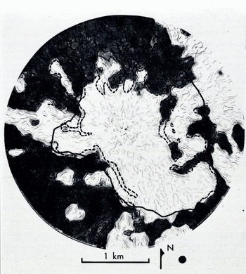
Fig. 1. Density-contour scan of ER TS image of South Cascade Glaaer basin. The heavy dark line is the basin outline. Areas determined tu be snow free using the ERTS data ore shaded. The snow tine as determined from ground and aerial photography is dashed. The black dot indicates the resolution element of the scanning microscope and represents a circle 84 m in diameter. ERTS image 1394-18311-5 (11 August 1973).
Resolution
A key to the usefulness of space images is resolution. The resolution of the ERTS MSS system is generally considered to be about 100 m, although under ideal conditions and with high contrast between objects, resolution is sometimes as high as 70 m. Snow lines in mountainous areas are intricate, and there is often high contrast between snow and rock or vegetation, and thus snow cover provides an ideal test of resolution. The snow line is routinely mapped from ground or aerial photographs in the South Cascade Glacier basin (lat. 48° 22’ N., long. 121° 03’ W.) for several dates during a typical melt season to help relate water input and oui How from the basin. This basin is approximately 6 km2 in area, and mass-balance data are compiled using a 100 m grid—in effect, a 100 m resolution. Snow outlines were drawn using ERTS images for several dales and by various methods. The simplest technique is to trace the snow line visually from optically enlarged images. This method is subjective as the observer must mentally estimate a line of equal density (grey tone) or sharp gradient in density.
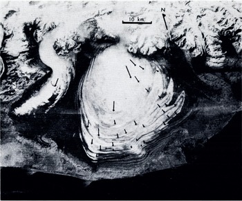
Fig. 2. Malaspina Glacier with 10 year velocity vectors superimposed. Vectors were determined by direct comparison of an ERTS image with a previous map compiled from aerial photographs. ERTS image 1420-20102-6 ( 16 September 1973).
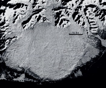
Fig. 3. Malaspina Glacier with new snow and a sun angle of 14° above the horizon. ERTS image 1204-30120-6 (12 February 1973).
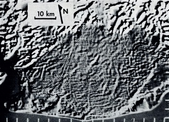
Fig. 4. Enhancement of February ERTS image of Malaspina Glacier. A positive superimposed with its negative, but slightly offset, with greatly enhanced contrast, highlights slight tonal variations. ERTS image 1204-20120 (12 February 1973).
A more objective method is through the use of a density-contour producing microscope (scanning densitometer). Several South Cascade images were also analyzed using this equipment. Although the machine can give an objective density contour, one must subjectively select the contour that most accurately represents the snow line. A density contour scan and the contour chosen as the most representative of the snow line are shown in Figure 1. The aperture (resolution element) of the microscope used to produce these contours was 25 μπη which represents 84 m on the ground, and is shown on the enlarged product as a dot. An aperture equivalent to 42 in was tried, but this resulted in a very noisy scan, showing that the image resolution was exceeded. Direct comparison of the density-contour snow line with the snow line drawn from ground and aerial photography is also shown in Figure 1. Generally the snow lines produced from the space image are smoother, as is to be expected, but values for the final snow-cover area agree well. Increased resolution could be obtained with the use of digitized images, but this requires more sophisticated equipment and more costly and difficult analysis.
Thus, we can state that in a basin where a 100 m (1 ha) resolution is adequate, useful snow-line or accumulation area data can be obtained from ERTS. Of course, conventional aerial photography can offer much better resolution. The advantages of ERTS are: (1) a virtually distortion-free orthographic view is produced, which simplifies data transfer to maps, (2) due to the large areal coverage of ERTS, many glaciers or large glaciers can be analyzed, and (3) because of the four channels, various methods of color enhancement or multi-spectral analysis can be used.
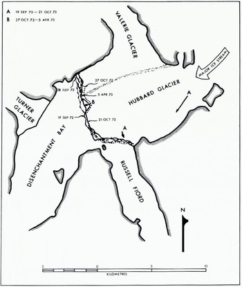
Fig. 5. Terminus positions of the Hubbard Cinder as determined from several ERTS images. Terminus displacement vector B is from 27 October 1972 to 5 April 1973 and surface velocity vectors A from 19 September 1972 to 21 October 1973.
Glacier Movement
The regional coverage that ERTS imagery provides is advantageous for other reasons. The Malaspina Glacier (lat. 60° 00’ N., long. 140° 40’W.) is about 50 km across. Aerial photographs of the glacier taken in 1962 were mosaicked together and the folded moraine positions meticulously plotted by Austin Post. ERTS images from 1972 were enlarged and compared directly to the 1962 map, a very quick and relatively easy task. The resulting 10 year velocity vectors are shown superimposed on a slightly more recent 1973 image (Fig. 2).
Surface And Bedrock Features
An image taken oi the Malaspina Glacier in February 1973, with a sun elevation of 14° and a uniformly reflecting surface of new snow, shows very slight slope changes as subtle tonal variations (Fig. 3). These tonal variations can be accentuated by first superimposing a negative and positive of the same image, then offsetting the images slightly and subsequently enhancing the contrast. This was done on an electronic console (Reference Evans and SerebrenyEvans and Serebreny, 1973), and the results are shown in Figure 4. A number of linear features are apparent which have no obvious relation to moraines or other known surface features.
The thickness of the central part of the Malaspina Glacier ranges from 500 to 1 000 m (Reference Allen and SmithAllen and Smith, 1953) and surface velocities are on the order of 2 to 300 m/year as determined by a map and ERTS image comparison. The wavy patterns and lineaments seen in the enhanced ERTS version are only surface features, but may be a reflection of the basal features, and perhaps can be interpreted as subglacial stream beds or differential erosion of geologic structures or formations. Thus they may relate to bedrock roughness elements, and hence subtly reflect the subglacial topographic relief.
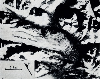
Fig. 6. ERTS image of Tweedsmuir Glacier. ERTS image 1471-19520 [6 November 1973).
Terminus Changes
Successive ERTS images can be used to determine short-term changes in terminus position and shape. The Hubbard Glacier (lat. 60° 05’ N., long. 139° 25’ W.), a tidal glacier in south-east Alaska, is about 100 km long and has recently attracted attention because of its slow advance across the mouth of the Russell Fiord. If the 200 km2 fiord were blocked, it would become a fresh-water lake which would either have an outlet at the opposite end or might periodically burst out through Hubbard Glacier (Post and Mayo, 1971). The glacier has been slowly advancing since 1895, and by 1970 bad come within 400 m of closing the fiord. Figure 5 shows terminus positions for several dates as determined from ERTS images in 1972 and 1973, and indicates that the advance has at least temporarily ended. A minimum distance of ice advance between 27 October 1972 and 5 April 1973 was 600 m, as an embayment in the terminus was closed in that time. Surface displacements of 600 and 1 800 in from 19 September 1972 to 21 October 1973 were also measured directly from the ERTS images.
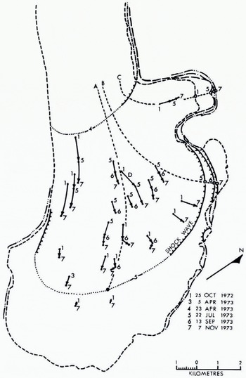
Fig. 7. Fig. 7. Tweedsmuir Glacier. Arrows tire surface velocity sectors; numbers by dots give the time interval. Shock-wave velocities were determined along lines A, B and C. All information here taken solely from ERTS images by L. R. Mayo, U.S. Geological Survey.
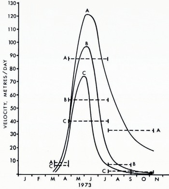
Fig. 8. Fig. 8. Shock-wave velocities along three longitudinal lines of Tweedsmuir Glacier during surge. Dashed lines are measured values, solid lines are inferred. Refer to Figure 7 for locations.
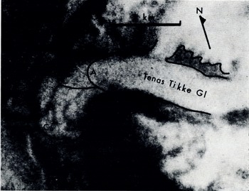
Fig. 9. A spectacular surge of the Tenas Tikke Glacier advanced the terminus i km before September 1972 (B) and an. additional 2 km by September 1973 (C). (A) is the pre-surge position of the terminus of the glacier. ERTS image 1416-19480 (12 September 1973).
Glacier Surges
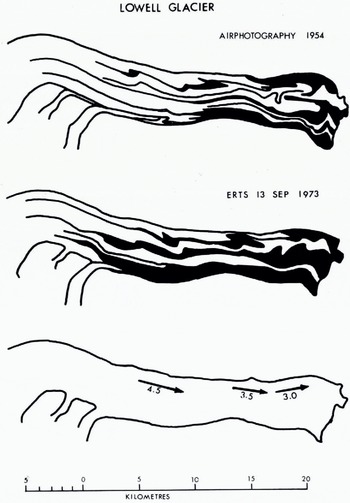
Fig. 10. Fig. 10. Surge displacements measured on the Lowell Glacier by comparison of ERTS images to previously drawn maps, which were compiled from aerial photographs.
The resolution and period of ERTS should allow useful lime-lapse data to be obtained before, during, and after glacier surges. The Tweedsmuir Glacier, (Fig. 6) (lat. 59° 40’ N., long. 138° 10’ W.), was noted to be surging during an aerial photographic flight in September 1973. Analysis of several ERTS images taken from October 1972 through November 1973 was undertaken by L. R. Mayo; these data are presented in Figures 7 and 8. The technique used for this analysis was to compare sequential photographic enlargements; Figure 8 shows measured and inferred shock-wave velocities in the terminal region. The inferred velocities were determined by drawing smooth curves that pass through the average displacement rates. The shock wave, near the center of the glacier, advanced at an average rate of 88 m/d from 23 April to 22 July 1972, at least an order of magnitude faster than the actual ice velocity. Although actual crevasses can rarely be seen on ERTS images, a darkening of the surface indicates a greater number of crevasses. During the surge the darkening proceeded up glacier 40 km in less than 180 d, at a rate of some 220 m/d. This and the location of the first noticeable shock wave in March and April indicate the surge began somewhere between 40 and 55 km from the head of the 70 km long glacier.
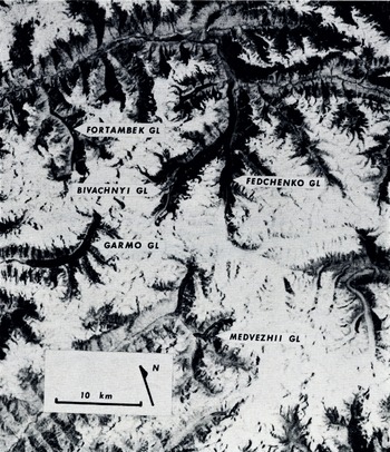
Fig. 11. ERTS image of Pamirs of Soviet Union. This image shows Lednik Medvezhiy after just completing a surge. Six surge-type and 16 glaciers with indistinct surge features hive been identified on this image. ERTS image 1354-05224-7 (l2 July 1973).
Another surge, that of the Tenas Tikke Glacier (lat. 59° 10’ N., long. 137° 00’ W.), was first noticed in an aerial photographic flight in September 1972. At that time it was supposed that this surge was just about finished after an advance of about 1 km from a previous length of 10 km. The 1973 aerial photographic flight showed the Tenas Tikke to have continued its advance an unexpected 2 km farther. At approximately the same time, ERTS imagery of the area was produced and the additional advance was very apparent (Fig. 9).
Another example in which surge displacements were easily determined through the use of ERTS data is that of the Lowell Glacier (lat. 60° 18’ N., long. 138° 51’ W.). The Lowell Glacier surged in 1968-70. A map of the medial-moraine pattern had been made before the surge from a mosaic of aerial photographs. A new map made directly from ERTS enlargements and compared to the earlier map allowed displacement vectors to be determined (Fig. 10).
The near-global coverage capability of ERTS is another great advantage. Figure 11 is a part of an image taken 12 July 1973 over the Pamirs of the Soviet Union (image center lat. 38° 57’ N., long. 72° 06’ W.) and is a good example of this capability. In this image Ledniki Medvezhiy is nearing the completion of a surge and a small surge-dammed lake is visible. Six other surging-type glaciers have been identified in this image including Ledniki Fortambek, Garmo, and Bivachnyy. The Bivachnyy shows characteristic moraine loops, and based on comparisons of similar glaciers in Alaska such as the Black Rapids Glacier (tat. 63° 30’ N., long. 146° 30’ W.) it is predicted that the Bivachnyy will surge within a few years with an ice displacement of about 2 km. At least 16 other glaciers on this image show surging characteristics.
Conclusions
ERTS images offer several advantages over other available methods for observing glaciers. A regional view is offered and large glaciers and ice caps that previously required tedious compilation of photographs into mosaics can now be seen on one frame. Features that are very subtle, but large, are often lost in the process of constructing mosaics. Furthermore, ERTS images are taken at times when aerial photography is not usually taken; for instance, under conditions of complete snow cover and low sun angle; these two factors often accent subtle regional topographic features. The repetitive coverage that ERTS offers is also useful in monitoring dynamic phenomena, the only requirement being that the changes observed exceed the resolution of the ERTS data. Finally, the near-global coverage that the ERTS system provides has obvious advantages.
The examples used in this paper illustrate only some of what has been done. To date the volume of data that ERTS has produced is much greater than has been utilized. Problems of data acquisition and distribution presently exist, but improvement is expected.
A major step in the data analysis not discussed here, but presently being undertaken, is computer processing of digital tapes. Images are available in the form of four reels of magnetic tape per set of four bands of one image. The computer-compatible tape format for ERTS images offers the advantages of maximum resolution and the greater analytical possibilities from computer processing of data.
Discussion
C. W. M. SWITHINBANK: ERTS coverage is not world-wide. Unfortunately neither ERTS-1 nor ERTS-B are programmed for even one-time coverage of all the land between latitudes 8i°N. and 81°S.
R. S. WILLIAMS, JR: Over the two years of global data acquisition by ERTS-1 the first priority was given to data acquisition by the 322 ERTS-1 principal investigators under contract to NASA. After their needs were satisfied NASA endeavored to provide one-time coverage of the entire world. However, certain areas of the world which are important in the raising of crops, such as China and Russia turned out to have higher priority, and therefore received more frequent coverage, than other areas. Acquisition of data imagery for these areas on a repetitive basis precluded coverage of other parts of the world which had no such coverage priority. It is interesting to note that this data-acquisition program was created late in the ERTS-i program to satisfy an internal U.S. Government (NASA, Department of Agriculture, and other agencies) project. This project, which includes discrete cooperation with other nations, is called LACIP (Large Area Crop Inventory Program). [Note added after Symposium: The LACIP is now included in an ERTS-B program (in addition to the 93 approved experiments) as one of several “ASVT” (application systems verification tests). It is estimated that over 70% of the total tape-recorder capacity on ERTS-B will therefore be devoted to the repetitive global crop inventories.]
It is hoped that NASA, with ERTS-B, will again return to the original lofty and worthy objectives of ERTS-1 and also to try to achieve at least one-time coverage of all land areas of the world, including the Antarctic. This is particularly important because the ERTS system represents the most important contribution yet made to all the peoples of the world from space technology. It is the only space project which at least began as a totally civilian, non-military endeavour.
W. F. BUDD: Have you been able to use overlapping ERTS images in stereo to obtain elevation contours?
R. M. KRIMMEL: We have not used this in our own studies, it has been attempted by others though.
J. MACDOWALL: Stereo can be seen over the Rocky Mountains, and false stereo has been noted by E. Langham as an easy way to observe differential sea-ice movement.
WILLIAMS: NASA applies 14 corrections to ERTS (MSS) imagery, thereby producing a distorted stereo model, unusable for topographic mapping. In Iceland, where significant sidelap of adjacent images (successive days) is the case, good stereo can be achieved. However, relative height measurements taken on Hcröubrciö, a table mountain in north-east Iceland which stands 1 000 m above the surrounding terrain, permit 10 contours to be drawn or one each 100 m. This appears to be the potential capability of ERTS-1.


