


1. Introduction
Although only ~1% of the world's glaciers have been observed to surge (Jiskoot and others, Reference Jiskoot, Boyle and Murray1998; Sevestre and Benn, Reference Sevestre and Benn2015), the interest and significance of surge-type glaciers extend far beyond their number because of the questions they raise about glacier dynamics in general. Why should some glaciers oscillate between slow and fast flow while the majority do not? Why are surge-type glaciers common in some regions but not others? Is surging contingent upon particular circumstances, or general dynamic or energetic principles? Is there a single explanation for all surges, or could multiple causes lead to similar oscillatory behaviour? Answering these questions is challenging due to the sheer diversity of surge-type glaciers. Surges can occur on land-terminating and tidewater glaciers, cirque glaciers, valley glaciers and ice streams, and on glaciers with temperate or polythermal regimes. They exhibit a wide range of cycle lengths and amplitudes, possibly forming a continuum with non-surging glaciers (Herreid and Truffer, Reference Herreid and Truffer2016). Surges may initiate in glacier accumulation or ablation zones and propagate up- or down-glacier, or both (Fowler and others, Reference Fowler, Murray and Ng2001; Cuffey and Paterson, Reference Cuffey and Paterson2010; Sevestre and others, Reference Sevestre2018).
Partly as a consequence of this diversity, numerous mechanisms have been proposed to explain glacier surging behaviour (e.g. Budd, Reference Budd1975; Clarke, Reference Clarke1976; Clarke and others, Reference Clarke, Nitsan and Paterson1977; Kamb and others, Reference Kamb1985; Fowler, Reference Fowler1987a; Fowler and others, Reference Fowler, Murray and Ng2001). Many of these invoke specific bed types, thermal regimes or drainage system configurations, and therefore can only explain part of the spectrum of observed surging behaviour. Global- and regional-scale analyses, however, show that surge-type glaciers occur within well-defined climatic envelopes, and exhibit consistent geometric characteristics regardless of the thermal regime (Clarke and others, Reference Clarke, Schmok, Ommanney and Collins1986; Jiskoot and others, Reference Jiskoot, Murray and Boyle2000; Sevestre and Benn, Reference Sevestre and Benn2015). This hints that a single set of physical principles underlies all surging behaviour, irrespective of differences in detail. A first attempt to identify these principles was made by Sevestre and Benn (Reference Sevestre and Benn2015), who sketched the outlines of a general theory of surging based on the relationship between glacier mass and enthalpy budgets. In this paper, we present a quantitative development of the theory using a simple lumped model based on the work of Fowler (Reference Fowler1987a) and Fowler and others (Reference Fowler, Murray and Ng2001). We compare model output with observed relationships between glacier dynamics, climate and geometry, and explore the implications of the theory for understanding the dynamic behaviour of the whole spectrum of glacier types.
2. Observations
The most striking fact about the occurrence of surge-type glaciers is that most are found within well-defined geographical clusters. Notable clusters exist in Alaska-Yukon, West Greenland, East Greenland, Iceland, Svalbard and Novaya Zemlya (collectively termed the ‘Arctic Ring’ by Sevestre and Benn, Reference Sevestre and Benn2015); High-Arctic Canada; parts of the Andes; and the Pamir, Karakoram and Tien Shan ranges of central Asia (e.g. Hewitt, Reference Hewitt1969; Post, Reference Post1969; Meier and Post, Reference Meier and Post1969; Osipova and others, Reference Osipova, Tchetinnikov and Rudak1998; Jiskoot and others, Reference Jiskoot, Luckman and Murray2002, Reference Jiskoot, Murray and Luckman2003; Copland and others, Reference Copland, Sharp and Dowdeswell2003; Fischer and others, Reference Fischer, Rott and Björnsson2003; Yde and Knudsen, Reference Yde and Knudsen2007; Kotlyakov and others, Reference Kotlyakov, Osipova, Tsvetkov and Jacka2008; Citterio and others, Reference Citterio, Paul, Ahlstrom, Jepsen and Weidick2009; Copland and others, Reference Copland2009; Grant and others, Reference Grant, Stokes and Evans2009; Copland and others, Reference Copland2011). Sevestre and Benn (Reference Sevestre and Benn2015) conducted a global analysis of surge-type glacier distribution, using a new database of all known surges in conjunction with the Randolph Glacier Inventory (RGI Consortium, 2017) and ERA-I climatic data. Because of the large size of ERA-I cells (0.75° × 0.75° latitude and longitude), the climatological data were indicative, and not representative of actual conditions experienced by each glacier, especially in areas of high relief. However, the analysis revealed that surge-type glaciers preferentially occur within distinct climatic environments (Fig. 1). Surge-type glaciers are almost entirely absent from the warmest and most humid glacierized ERA-I cells, and very rare in the coldest and driest. In contrast, ERA-I cells with intermediate climates commonly contain concentrations of surge-type glaciers in addition to non-surging glaciers. The analysis also showed that in all geographic clusters, surge-type glaciers tend to have greater areas, greater lengths and lower gradients than non-surging glaciers (Fig. 1). This corroborates the results of within-cluster analyses, which identified strong associations between surging behaviour and geometric characteristics (e.g. Clarke and others, Reference Clarke, Schmok, Ommanney and Collins1986; Clarke, Reference Clarke1991; Hamilton and Dowdeswell, Reference Hamilton and Dowdeswell1996; Jiskoot and others, Reference Jiskoot, Boyle and Murray1998, Reference Jiskoot, Murray and Boyle2000, Reference Jiskoot, Murray and Luckman2003; Björnsson and others, Reference Björnsson, Pálsson, Sigurđsson and Flowers2003; Copland and others, Reference Copland, Sharp and Dowdeswell2003; Grant and others, Reference Grant, Stokes and Evans2009). Some studies additionally revealed a tendency for surge-type glaciers to occur on particular substrates, particularly weak sedimentary rocks or fault zones (Post, Reference Post1969; Truffer and others, Reference Truffer1999; Jiskoot and others, Reference Jiskoot, Murray and Boyle2000; Björnsson and others, Reference Björnsson, Pálsson, Sigurđsson and Flowers2003).
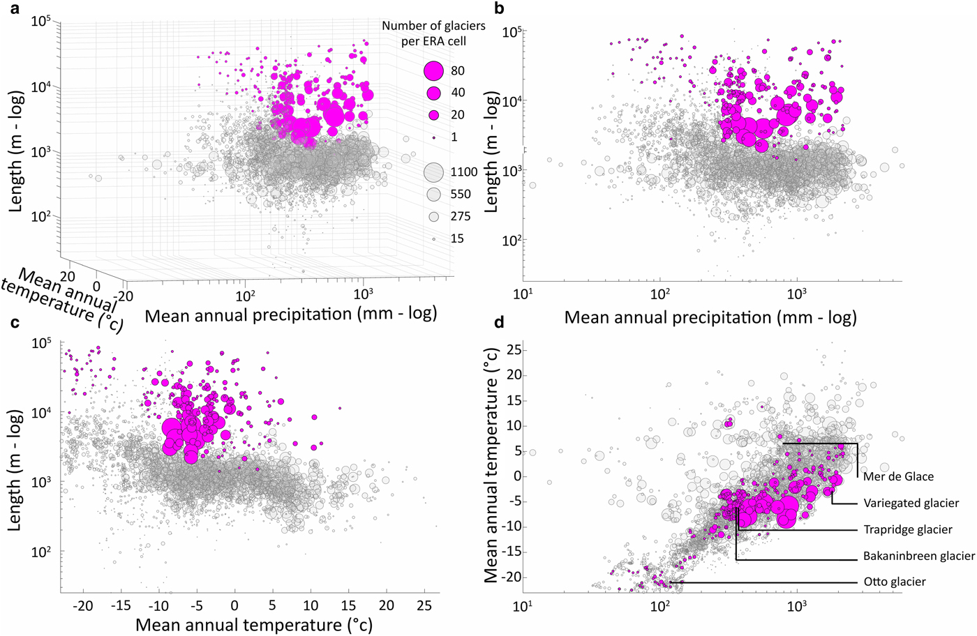
Fig. 1. Global-scale associations between surge-type glaciers and geometric and climatic variables. Circles show the number of surge-type (magenta) and non-surge-type (grey) glaciers per ERA-I cell. (a) Three-way plot of ERA-I mean annual temperature, annual precipitation and mean glacier length. (b) Mean glacier length vs precipitation. (c) Mean glacier length vs temperature. (d) Temperature vs precipitation, showing the location of Variegated Glacier (Alaska), Trapridge Glacier (Yukon), Bakaninbreen (Svalbard) and Otto Glacier (Ellesmere Island, Canada).
3. Theories of surging
Many surge mechanisms have been proposed over the years, including triggering by external factors such as earthquakes or landslides (Tarr and Martin, Reference Tarr and Martin1914; Gardner and Hewitt, Reference Gardner and Hewitt1990); episodic self-regulation (Miller, Reference Miller1973); transitions from frozen to temperate basal conditions (Clarke, Reference Clarke1976; Fowler and others, Reference Fowler, Murray and Ng2001; Murray and Porter, Reference Murray and Porter2001); switches in the configuration of the subglacial drainage system (Kamb and others, Reference Kamb1985; Kamb, Reference Kamb1987; Fowler, Reference Fowler1987a); interactions between till deformation and drainage efficiency (Clarke and others, Reference Clarke, Collins and Thompson1984); propagating waves of till failure and healing (Nolan, Reference Nolan2003); pulsed englacial water storage (Fatland and Lingle, Reference Fatland and Lingle2002; Lingle and others, Reference Lingle and Fatland2003); and topographic controls (Flowers and others, Reference Flowers, Roux, Pimentel and Schoof2011; Abe and others, Reference Abe, Furuya and Sakakibara2016; Lovell and others, Reference Lovell, Carr and Stokes2018). Fully developed numerical models of surging, however, have tended to draw from a relatively small number of ingredients, namely, an effective pressure-dependent friction law, thermodynamic feedbacks, switches in drainage system configuration, and the relationship between balance flux and stable flow modes. These are discussed in turn below.
3.1 Effective pressure-dependent friction law
The relationship between basal velocity u and shear stress τ is strongly influenced by the presence of pressurized water at the bed, either via lowering the yield strength of subglacial till or increasing the extent of cavities between ice and bed (Cuffey and Paterson, Reference Cuffey and Paterson2010). When the effective pressure N (normal ice pressure p i minus basal water pressure p w) is large, velocity increases with stress, but as N decreases, high velocities can occur when basal stress is small (Lliboutry, Reference Lliboutry1968; Fowler, Reference Fowler1987b; Schoof, Reference Schoof2005). The possibility that effective pressure-dependent friction laws could lead to flow instabilities was first raised by Lliboutry (Reference Lliboutry1968), and this idea lies at the heart of most theories of surging, in which increases in basal water pressure trigger glacier acceleration (e.g. Budd, Reference Budd1975; Fowler, Reference Fowler1987a; Fowler and others, Reference Fowler, Murray and Ng2001; Kyrke-Smith and others, Reference Kyrke-Smith, Katz and Fowler2014).
3.2 Thermodynamic feedbacks
Feedbacks between ice velocity and frictional heating are a form of instability characteristic of stress-driven flows with temperature-dependent viscosity, and have been invoked as a possible cause of surges for well over half a century (e.g. Ahlmann, Reference Ahlmann1953; Robin, Reference Robin1955; Clarke, Reference Clarke1976; Clarke and others, Reference Clarke, Nitsan and Paterson1977; Murray and others, Reference Murray, Strozzi, Luckman, Jiskoot and Christakos2003). Velocity-heating feedbacks may manifest as warming and softening of cold ice (thermal runaway), water accumulation and enhanced basal motion at the beds of temperate glaciers (hydraulic runaway), or thawing and build-up of water at the beds of polythermal glaciers (a combination of the two). There is strong evidence that thermodynamic feedbacks triggered surges of small, relatively thin Arctic glaciers during the Little Ice Age (Lovell and others, Reference Lovell2015; Sevestre and others, Reference Sevestre and Benn2015).
Both thermal and hydraulic runaway mechanisms are incorporated in the surge model of Fowler and others (Reference Fowler, Murray and Ng2001), which exhibits cycling between cold-bedded (quiescent) and warm-bedded (surging) states. In addition, thermodynamic feedbacks are key elements of several models of ice flow instabilities (e.g. Yuen and Schubert, Reference Yuen and Schubert1979; MacAyeal, Reference MacAyeal1993; Fowler and Johnson, Reference Fowler and Johnson1995; Fowler and Schiavi, Reference Fowler and Schiavi1998; Tulaczyk and others, Reference Tulaczyk, Kamb and Engelhardt2000; Calov and others, Reference Calov, Ganopolski, Petoukhov, Claussen and Greve2002; Jay-Allemand and others, Reference Jay-Allemand, Gillet-Chaulet, Gagliardini and Nodet2011; van Pelt and Oerlemans, Reference Van Pelt and Oerlemans2012; Kyrke-Smith and others, Reference Kyrke-Smith, Katz and Fowler2014; Feldmann and Levermann, Reference Feldmann and Levermann2017).
3.3 Hydrologic switching
Drawing upon an unparalleled set of observations of the 1982–1983 surge of Variegated Glacier, Alaska, Kamb and others (Reference Kamb1985) argued that surges of temperate glaciers could occur due to switching of the basal drainage system from efficient conduits to an inefficient ‘linked cavity’ system. Inefficient drainage encourages high basal water pressures (low N) whereas efficient drainage reduces water storage (high N). Thus, switches in drainage system type could underpin oscillations between ‘slow’ and ‘fast’ modes of flow. This mechanism is at the core of Fowler's (Reference Fowler1987a) model of surging, which exhibits switches in drainage system type in concert with cyclic changes in ice thickness and velocity. The model assumed constant subglacial discharge, and did not consider variations in meltwater production via frictional heating or other sources.
Variations in meltwater production and discharge were incorporated in the surge model of Fowler and others (Reference Fowler, Murray and Ng2001). Thermal and hydraulic runaway processes lead to thawing and water accumulation in an inefficient Darcian-type drainage system during late quiescence, then this water is instantaneously removed from the system when N approaches zero. Rapid drainage at low N was justified by invoking efficient drainage through connected ‘blisters’, or regions of ice–bed decoupling (‘blister flux’), following Stone and Clarke (Reference Stone and Clarke1996). The model of Fowler and others (Reference Fowler, Murray and Ng2001) did not, however, include an explicit representation of such an efficient drainage system.
3.4 Balance flux vs flow mechanisms
The balance flux (the integrated surface mass-balance upstream of a specified flux gate on the glacier) determines the ice discharge required for a glacier to remain in dynamic equilibrium with climate. Budd (Reference Budd1975) argued that combinations of balance flux and velocity–friction relationships underpin the distinction between ‘ordinary’, ‘fast’ and ‘surging’ glaciers. On ‘ordinary’ glaciers, the balance flux is consistent with a slow flow mode, in which basal velocity and stress increase together, allowing glacier geometry to evolve to achieve a steady state. ‘Fast’ glaciers, in contrast, have a sufficiently high balance flux to sustain the flow in the fast mode, with high velocities and low effective pressures and basal stress. Surging glaciers oscillate between fast and slow modes, to discharge the balance flux over long periods of time.
Sevestre and Benn (Reference Sevestre and Benn2015) built upon this idea, arguing that both mass flux and enthalpy balances have to be satisfied for a glacier to remain in a stable steady state. For an incompressible ice mass, enthalpy relates to the temperature and liquid water content of the ice (Aschwanden and others, Reference Aschwanden, Bueler, Khroulev and Blatter2012). Enthalpy is gained at the glacier bed from the geothermal heat flux plus frictional heating (expenditure of potential energy) associated with the ice flux. Enthalpy losses occur by the dissipation of heat by conduction and loss of meltwater from the system. Ice flow rates depend sensitively on ice temperature and water storage at the bed, so for a glacier to maintain a steady flow, there must be a broad equality between enthalpy gains associated with the mass flux and enthalpy losses via conductive cooling and runoff. Sevestre and Benn (Reference Sevestre and Benn2015) postulated that under certain combinations of climate, geometry and bed geology, glaciers are unable to balance their mass and enthalpy budgets, and thus undergo mass and enthalpy cycles that manifest as quiescent and surge phases.
4. A general model of surging
4.1 Overview
We now construct a general model of surging, combining elements described above. Following Fowler (Reference Fowler1987a) and Fowler and others (Reference Fowler, Murray and Ng2001), we adopt a non-spatial lumped model. We choose a lumped approach in preference to investigating specific geometries in 2-D or 3-D, because we seek to identify and explore the principles underlying the behaviour of glaciers in general, independently of the details of particular cases. In addition, a lumped approach allows a thorough exploration of model parameter space, in keeping with our aim of understanding the combined influence of climatic and geometric parameters at the glacier population scale. We represent the ice as an inclined, parallel-sided slab with slope θ and characteristic thickness H measured normal to the bed (Fig. 2). Variables can be interpreted as averages over the accumulation zone of the glacier.
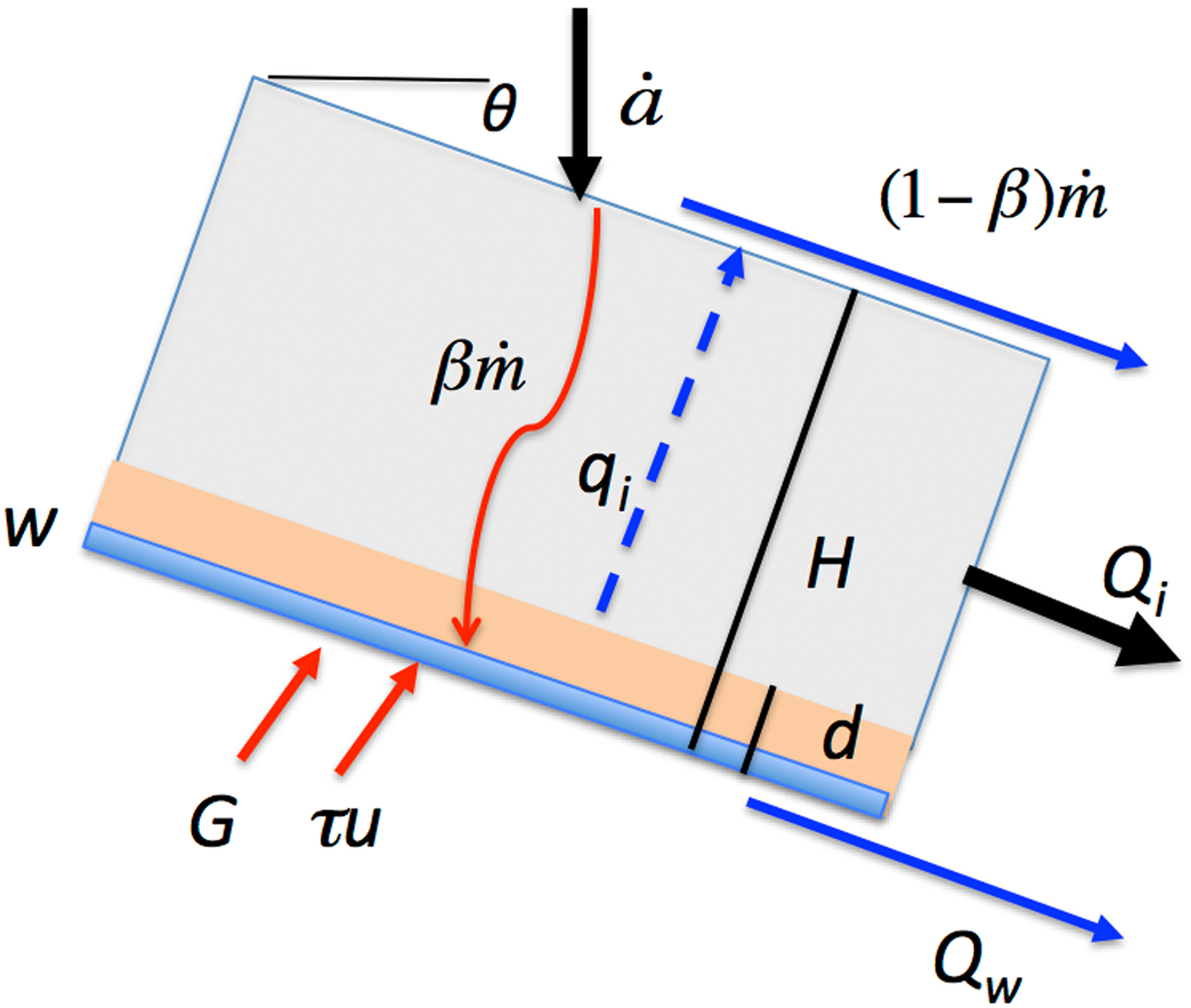
Fig. 2. Geometry of the lumped model, showing enthalpy sources (red) and sinks (blue). w is the depth of basal water and d is the thickness of the basal zone for which enthalpy is calculated. See text for other definitions.
Repeated surges represent periodic oscillations of the underlying dynamics of the glacier flow (Fowler, Reference Fowler1987a). The simplest system that can produce self-sustained oscillations is a pair of ordinary differential equations, here chosen to represent the evolution of ice thickness H and the enthalpy E in a thin layer spanning the basal ice and the ice–bed interface. This pair of ODEs represents the key principles at the heart of glacier dynamics: mass conservation and enthalpy conservation.

where $\dot{a}$ is the prescribed accumulation rate, $\dot{m}$
 is the net ablation rate (i.e. meltwater that is not refrozen or otherwise stored in firn), Q i is the ice flux, and l is the length (of the accumulation area strictly, though we assume this is proportional to the glacier length). τu is the frictional heating from sliding (τ is the basal shear stress and u the sliding speed), G is the geothermal heat flux, q i is the conductive cooling flux, Q w is the discharge rate of basal water, β is the proportion of surface melt that reaches the bed, ρ is the density and L is the latent heat of fusion. To simplify the calculations, we ignore the density difference between ice and water. This does not affect model physics, and given the approximate lumped nature of the model has a negligible impact on the results. The first, second and fifth terms on the right-hand side of (2) are enthalpy sources, and the third and fourth terms are enthalpy sinks. The final term on the right-hand side is water derived from the surface, which is an enthalpy source. For simplicity, we neglect viscous heating from deformation in the basal ice, which is generally very small compared to other terms (typically two orders of magnitude less than the geothermal heat flux for a unit thickness of basal ice).
We build the components of (1) and (2) from the following ingredients.
4.2 Mass and enthalpy fluxes
Net ablation is assumed to be linearly proportional to mean annual air temperature T a:

where DDF is a degree-day factor and T offset is the difference between mean annual temperature and the mean annual temperature below which there is no melting. We ignore seasonal cycles, so $\dot{m}$ is the mean annual melt rate.
Enthalpy E is related to basal temperature and water content according to:

where c p is the specific heat capacity of ice, d is the thickness of the basal layer (taken to be d = 10 m), T is the basal ice temperature, T m is the melting temperature (taken as constant at 0°C) and w is the average depth of water stored at the bed.
We scale the enthalpy variable such that negative values correspond to ‘cold content’ and positive values refer to water content. Since T is fixed at T m if w > 0 (temperate condition), and w = 0 if T < T m (cold condition), we can invert (4) to write

where E_ = min(E; 0) and $\displaystyle{{E_ +}}$ = max(E; 0). Because of the non-spatial nature of the model, the bed exists in either a cold or warm state, never a mixture of the two.
The ice flux Q i is taken to be

with the first term being the contribution from sliding, and the second term being the contribution from internal deformation using the shallow ice approximation. A and n are the coefficients in Glen's flow law.
The sliding velocity u is determined from a generalized Weertman friction law:

and we take basal shear stress to be equal to the driving stress τ = ρgHsinθ. The ice surface slope is set equal to the bed slope θ, which is a free input parameter in the model. N is the effective pressure and R is a constant roughness coefficient. This can be rearranged to write

Equation (8) adds effective pressure-dependent sliding to the model (section ‘Effective pressure-dependent friction law’). We choose this relationship in preference to more sophisticated approaches because it captures the essential relationships between u, τ and N while simplifying the algebraic structure of the model.
The conductive cooling term q i is approximated as a linear function of the temperature difference between the ice surface and the bed:

where k is the thermal conductivity of ice and T a is the mean annual air temperature (the subtraction of T m and the minus sign are to account for the fact that neither the base nor the surface of the ice may be warmer than the melting temperature, even if the air temperature is larger than that). Equation (9) assumes steady-state thermal conditions, which is reasonable because T a is held fixed in model runs and basal temperature T evolves very slowly.
4.3 The drainage system
Framing a satisfactory description of the basal drainage system is not entirely trivial. Previous models of surging have tended to circumvent the problem or adopt steady-state approximations of the system. However, a large body of observations shows that temporal variations in subglacial water recharge, storage and discharge play a key role in the dynamics of both surge-type and non-surge-type glaciers (e.g. Cuffey and Paterson, Reference Cuffey and Paterson2010), and this demands that any general theory of surging must address the issue of drainage system evolution. We approach the problem in two steps. First, we define a single-component drainage system in which water flux is a function of mean water depth w at the bed. This can be visualized as an inefficient, distributed system when w is small (e.g. flow of porewater in till or other subglacial aquifers, or along the ice–bed interface in a system of small, poorly-connected cavities), becoming more efficient and better connected as the amount of stored water increases (e.g. in a system of canals or well-connected cavities at the ice–bed interface). Discharge through this efficient distributed system is analogous to the ‘blister flux’ of Fowler and others (Reference Fowler, Murray and Ng2001).
Second, we define a two-component system that can include both a distributed component and subglacial R-channels or conduits. R-channels can potentially draw down water storage when w is high but also allow high water flux when w is small if supply is large. In the two-component system, both elements compete to discharge water, and typically one will dominate at the expense of the other. Our aim is not to provide an explicit picture of the drainage system, but to investigate the degree to which surging behaviour depends on how subglacial drainage adapts under different circumstances.
We assume that there is an inverse relationship between the average depth of stored water w and effective pressure N. For convenience we set:

where $\tilde{C}$ is a prescribed constant. The water depth w can represent water storage within a compressible layer of till, or within a film or system of cavities at the ice–bed interface; in all of these cases, one expects a (steady-state) relation of broadly this form (Hewitt, Reference Hewitt2011, Reference Hewitt2013). The effective pressure cannot exceed the ice pressure ρgH, so in terms of water depth and enthalpy, respectively, we replace (10) with

where $C = \rho L\tilde{C}.$
The single-component, distributed drainage system is defined by:

where ρgsinθ is the hydraulic gradient arising from the bed slope. $\tilde{K}w^\alpha$ is the hydraulic transmissivity, which varies with water film depth w. $\tilde{K}$
 thus represents the invariant components of conductivity (e.g. small-scale bed roughness, till porosity) and fluid viscosity. α is set to a relatively large value (5) to account for the idea that at low water volumes discharge is low, but at high volumes the discharge can increase rapidly. The water pressure component of the hydraulic potential gradient is neglected because it is a spatially variant property not readily incorporated in the present lumped model formulation.
The two-component system includes a second term representing water discharge in a conduit:

in which K c is a constant related to Manning's roughness coefficient, S is the cross-section area of conduits, spaced at width W c. The half power of the hydraulic gradient derives from the assumption of turbulent flow in a semicircular channel. The factor ϕ is introduced as a ‘fill-fraction’ to allow for the possibility of channels being only partially filled at times of falling discharge. According to (11), this happens when $\rho gHw \lt \tilde{C}$ (corresponding to the drainage system being at atmospheric pressure), and we therefore take

which makes flow in partially-filled channels proportional to the global water thickness w. Without this modification, a previously enlarged channel would unphysically continue to drain a large flux of water even when the supply drops off.
Channel cross-section area S evolves through time according to the kinematic condition:

$\tilde{A}$ is a rate factor analogous to A in Glen's flow law. The first term on the right-hand side represents channel enlargement by wall melting due to turbulent heat dissipation, the second term represents creep closure, and the third is a small opening term associated with wall melting driven by other heat sources (geothermal and frictional heat) or ice sliding over bed roughness elements (Schoof, Reference Schoof2010; Hewitt, Reference Hewitt2011; Werder and others, Reference Werder, Hewitt, Schoof and Flowers2013). We choose this approach over setting a minimum channel cross-section area since it allows the same Eqn (15) to hold all the time. Where two-component drainage is included in the model, (15) adds a third ordinary differential equation to the coupled system (1) and (2) (see Appendix).
The proportion β of surface melt that reaches the bed (Eqn (2)) can be set to zero or varied to represent surface-to-bed drainage through moulins nucleated on crevasses (cf. van der Veen, Reference Van Der Veen1998; Benn and others, Reference Benn, Kristensen and Gulley2009). The amount of surface-to-bed drainage depends on the extent of surface crevasses, which in turn is related to spatial phenomena (e.g. velocity gradients) that are not explicitly simulated. We assume that β is proportional to the ice velocity:
i.e. ice with a velocity less than u 1 is assumed to be uncrevassed and impermeable, whereas if velocity equals u 2 or above, the ice is pervasively crevassed and all net surface meltwater reaches the bed. This is the simplest possible formulation that allows the model to explicitly exhibit feedbacks between surface-to-bed drainage and ice dynamics.
Variables were scaled and non-dimensionalized prior to model implementation. Details are given in the Appendix and parameter values are listed in Table 1. The model is structurally similar to that of Fowler and others (Reference Fowler, Murray and Ng2001), which solved coupled ordinary differential equations for ice thickness H and effective pressure N, rather than H and E. Indeed, Fowler and others (Reference Fowler, Murray and Ng2001) defined N in a way that closely matches our definition of E. The main innovations in our model are: (1) partitioning of surface mass balance into accumulation and melt components to allow investigation of their influence on surging behaviour; (2) more detailed treatment of basal hydrology, particularly the introduction of a time-evolving two-component drainage system; and (3) incorporation of surface-to-bed drainage. In our model, subglacial discharge and drainage efficiency evolve in response to changing water sources and sinks, unlike the original hydrological switch model of Fowler (Reference Fowler1987a) in which discharge was assumed to be constant.
Table 1. Default parameter values, scales and dimensionless parameters
Due to the approximate, lumped nature of the model, the values of some constants have been rounded. The flow-law parameter A is taken to be a representative depth-averaged value (across the full ice thickness, since the place it enters is in the shallow-ice flux) and therefore smaller than the textbook value at 0°C.
5. Results
Model runs were conducted to find steady-state solutions of (1) and (2) for a range of values of accumulation $\dot{a}$ , mean annual air temperature T a, glacier length l, bed slope θ and the hydraulic conductivity parameter $\tilde{K}$
 . Variations in $\dot{a}$
 and T a were applied to explore the influence of climate on surging behaviour, variations in l and θ to explore the influence of geometry, and variations in $\tilde{K}$
 to examine the influence of bed properties, as a proxy for substrate type. Three variants of the model were employed: (1) single-component basal drainage, no surface meltwater input; (2) single-component drainage, possible surface meltwater input; and (3) two-component drainage, possible surface water input. The first case allows us to examine the impact of basal processes in isolation, the second to address the influence of surface water flux on a distributed drainage system, and the third to investigate systems where high-flux, low-storage states are possible. It should be noted that none of these cases is more or less ‘realistic’ than the others. Rather, our stepwise approach allows us to determine how different behaviours emerge as system components are added.
5.1 Single-component drainage, no surface water input
In the simplest form of the model, subglacial water discharge is calculated using (12) and the surface drainage parameter β is set to zero. Steady-state solutions (dH/dt) = (dE/dt) = 0 are either stable or unstable (oscillatory), depending on the combinations of accumulation and air temperature. On enthalpy–thickness phase portraits (Fig. 3), the line along which (dH/dt) = 0 (the H-nullcline) is always monotonic, whereas the E-nullcline (dE/dt) = 0 is multivalued for many combinations of parameters. Points where the nullclines cross represent steady-state solutions, which are stable if the crossover lies on the upper or lower branch of the E-nullcline, and typically unstable if it lies on the middle branch.
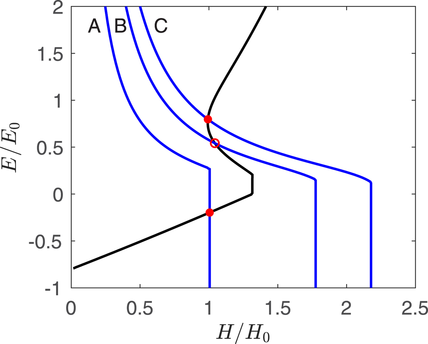
Fig. 3. Phase portrait of enthalpy E and ice thickness H, for three values of accumulation. The black line is the E-nullcline, on which dE/dt = 0, and the blue lines are the H-nullclines on which dH/dt = 0, with $\hat{T}_{\rm a}$ = −0.8, and $\dot{a}$
 = 0.23 (A), 0.4 (B) and 0.7 (C). Case B corresponds to Figure 4. The enthalpy and ice thickness scales are normalized with respect to reference values E 0 = 1.8 × 10⁸ J m−2 and H 0 = 200 m.
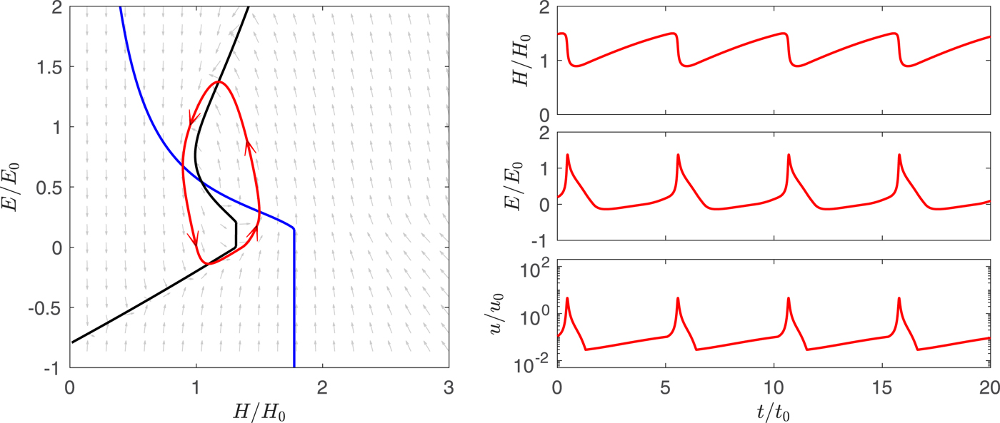
Fig. 4. An example solution of the model in a surging regime, corresponding to case B in Figure 3. Background arrows indicate the trajectory of E and H in the parameter space.
This is illustrated in Figure 3, which shows alternative positions of the H-nullcline associated with low (A), intermediate (B) and high (C) values of $\dot{a}$ . For low $\dot{a}$
 , the crossover lies on the lower branch; this represents a stable steady state with relatively thick ice, low enthalpy (cold basal ice) and low velocities. For high $\dot{a}$
 , the crossover lies on the upper branch and represents a stable steady state with relatively thin ice, high enthalpy (in the form of water at the bed) and high ice velocities. For the intermediate case, the crossover lies on the middle branch of the E-nullcline. Although there is a balance between enthalpy production (by geothermal and frictional heating) and enthalpy loss (by conductive cooling and drainage) at the crossover, this state is unstable to small perturbations because any small increase in ice thickness leads to an increase in heating that cannot be offset by enthalpy losses. This then leads to a positive velocity-heating feedback, and thereafter ice thickness, enthalpy and velocity undergo periodic oscillations (Fig. 4). Enthalpy and ice velocity are low during a long quiescent phase, during which ice thickness increases. In this particular case, enthalpy becomes negative (frozen bed conditions) during the quiescent phase. Increasing ice thickness and reduced conductive heat losses eventually thaw the bed and basal water accumulates, then velocity–frictional heating feedbacks trigger a rapid increase in basal water storage and sliding velocity. Finally, w rises high enough to allow rapid drainage, terminating the brief surge phase.
The position and shape of both nullclines vary depending on climatic ($\dot{a}$ , T a), geometric (l and θ) and hydraulic ($\tilde{K}$
 ) input values. For example, an increase in accumulation shifts the H-nullcline to the right but has no effect on the E-nullcline (Fig. 5a). This is because $\dot{a}$
 appears in Eqn (1) but not Eqn (2) or its components. With higher accumulation, the glacier occupies a stable steady state, with greater ice thickness and enthalpy than before. In contrast, a decrease in air temperature results in rightward shifts of the H-nullcline and the lower part of the E-nullcline (Fig. 5b). This is because decreasing air temperature increases net accumulation and thicker ice is needed to reduce conductive cooling to balance the enthalpy budget. The impact of increasing bed slope is shown in Figure 5c: the H-nullcline and the upper part of the E-nullcline are both shifted to the left. Other factors being equal, increasing bed slope increases both ice flux (6, 8) and Q w (12), so for steady state, H must decrease to balance increased drainage efficiency. Finally, a doubling of glacier length moves the H-nullcline to the right, but the upper part of the E-nullcline to the left (Fig. 5d). The resulting steady state is a thinner, higher enthalpy glacier, due to the impact of increased length on ice flux (1) and basal water discharge (2).

Fig. 5. The effect of changing parameters on the phase plane. The dotted lines show the default nullclines, with associated arrows showing the direction of trajectories. Solid lines show the effect of varying the given parameter. (a) Doubling accumulation; (b) doubling the difference between air temperature and the melting point; (c) doubling bed slope; (d) doubling glacier length.
Thus, depending on the combinations of $\dot{a}$ , T a, l and θ, glaciers can exist in a stable temperate state, a stable cold state or undergo periodic oscillations in H and E. Over the course of each surge cycle, the basal condition either cycles between cold and warm states or remains entirely temperate. Figure 6 shows the range of (normalized) accumulation and air temperature values associated with oscillatory behaviour, for one combination of l and θ.
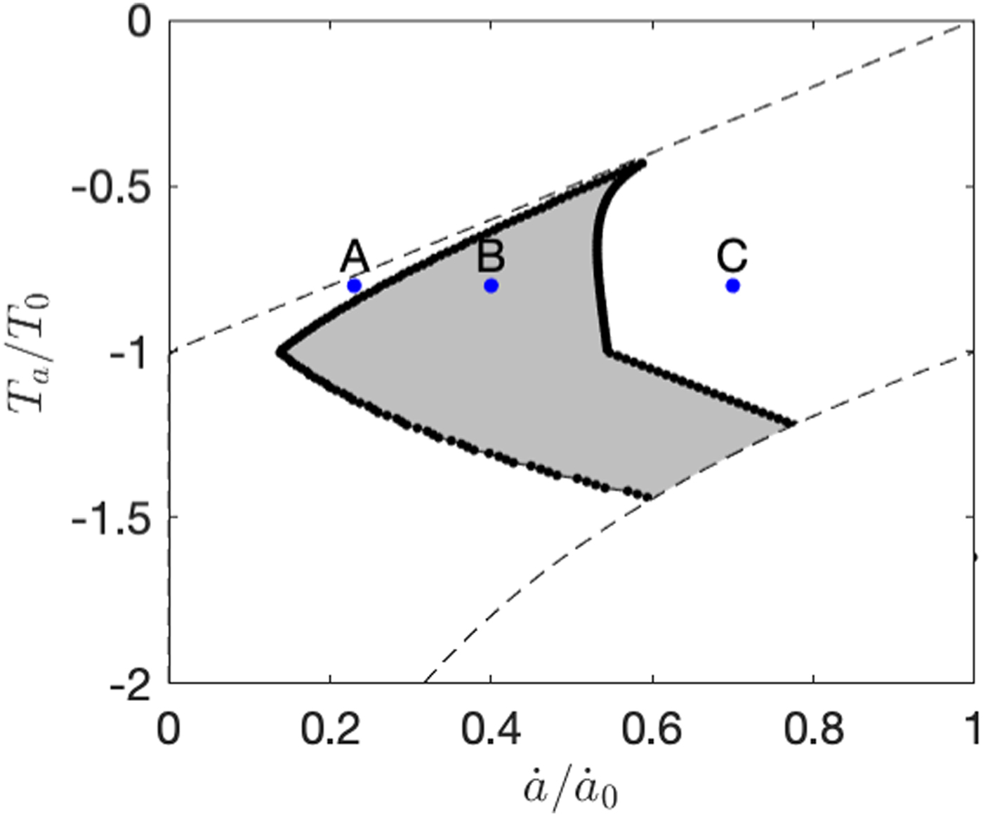
Fig. 6. Modelled surging regime (grey) as a function of accumulation and air temperature. (A), (B) and (C) correspond to the cases shown in Figure 3. The dashed lines bound the possible parameter space: the empty region top left is where $\dot{m} \gt \dot{a}$ , so glaciers cannot occur, and the empty region bottom right denotes humid–cold climate combinations that do not occur in nature.
Varying l and θ shift the position of the zone of oscillatory behaviour, such that an increase in glacier length or a decrease in slope allows surging behaviour in colder and drier climates (Fig. 7a). The oscillatory zone also shifts in response to changes in drainage system parameters. For example, a reduction of the hydraulic conductivity parameter $\tilde{K}$ to 10% of its default value expands the surging regime into the warm–humid end of the climate spectrum, whereas a tenfold increase in $\tilde{K}$
 reduces the extent of the surge regime, confining it to the cold–dry end of its default range. That is, less efficient drainage encourages surging behaviour in warmer, more humid climates, whereas more efficient drainage precludes it.
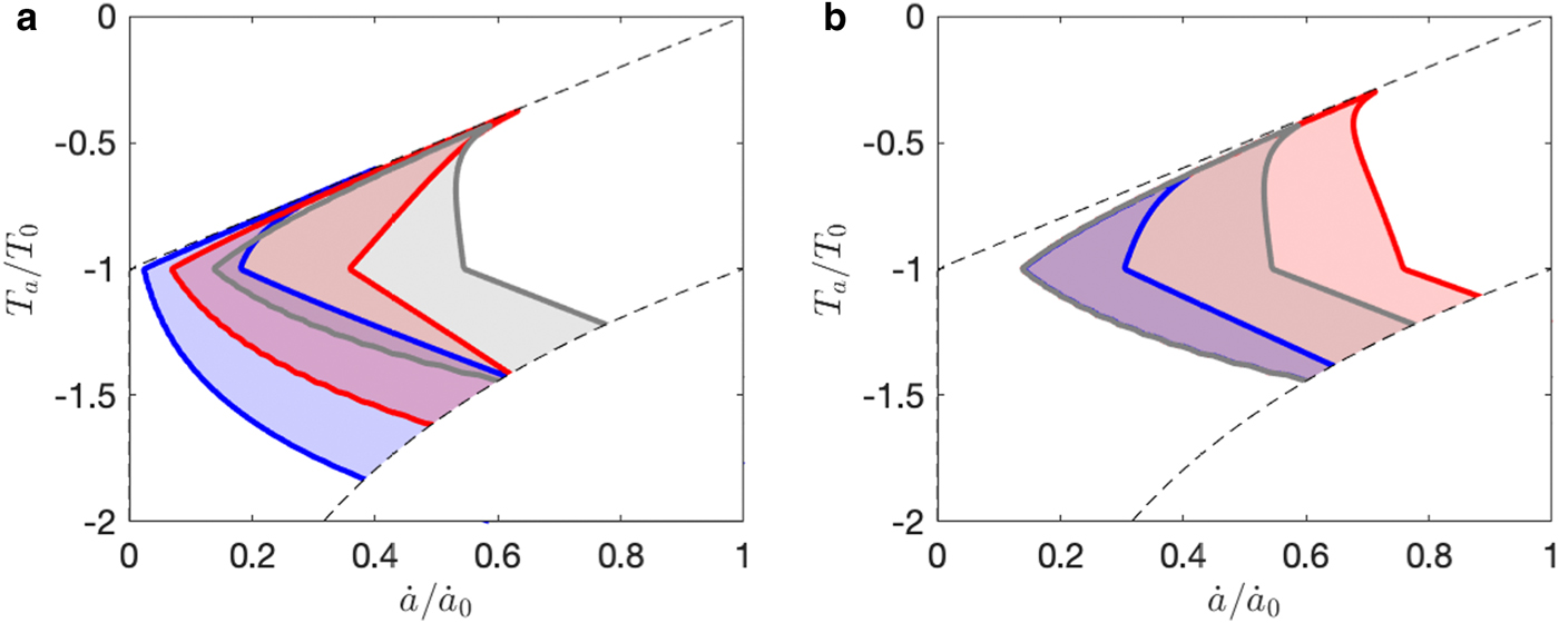
Fig. 7. (a) Surging regime for default parameters (grey), double the length (red) and half the slope (blue). (b) Surging regime for default parameters (grey), reducing the hydraulic conductivity constant $\widetilde{{K\;}}$ to 10% of its default value (red), and increasing $\tilde{K}$
 tenfold (blue).
Figure 8 shows the distribution of oscillatory behaviour for a single climate state ($\hat{\dot{a}}\; = 0.4$ ; $\hat{T}_{\rm a} = -0.8$
 ) for varying l and θ, representing glaciers with a range of geometries within a climatically-uniform region. For this case, very gently sloping glaciers have stable steady states that are thick and warm-based, while steeper glaciers find stable steady states that are thin and cold. Oscillatory behaviour occurs for intermediate slopes, over a range that increases with glacier length.
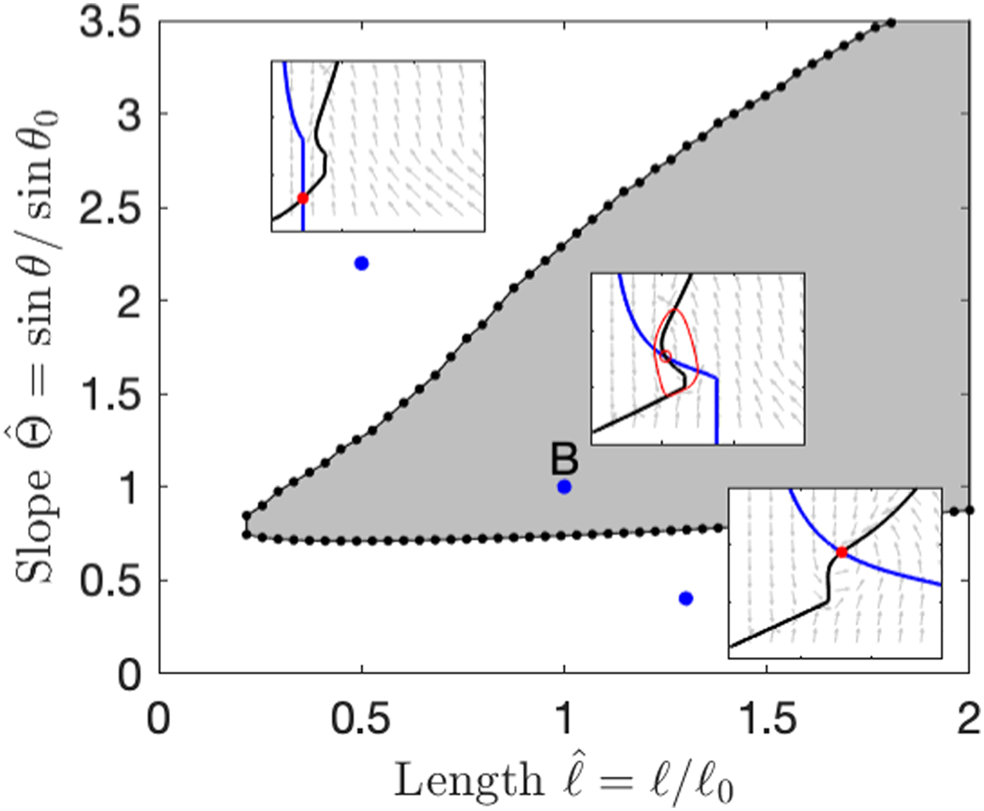
Fig. 8. The parameter regime in which oscillatory (surging) states occur for fixed climate variables, T a = −0.8, $\dot{a}$ = 0.4, and variable length and slope, with examples of the phase plane for the parameter values indicated by blue dots.
5.2 Single-component drainage system, with surface water input
Routing surface meltwater to the glacier bed by activating the β(u) function (16) modifies the behaviour of oscillatory glaciers, regardless of the thermal regime. Depending on the chosen input parameters, activating surface water input impacts glacier dynamics in different ways. First, the addition of surface-to-bed drainage can stabilize the flow, as shown in Figure 9. In this case, the steady-state solution is oscillatory in the absence of surface water input, because rates of basal meltwater production (from geothermal and frictional heating) and water discharge (12) are mismatched. The glacier consequently undergoes repeated cycles of mass and enthalpy build-up and release. Activating the β(u) function routes surface water to the bed, allowing much larger subglacial water fluxes, which in turn sustain sliding at a rate that matches the balance flux. A stable steady state is now possible, with thinner, faster-moving ice facilitated by surface meltwater penetration. In terms of the phase plane (Fig. 9b) this is reflected in a change in the position of the E-nullcline, so the crossover with the H-nullcline now lies on the upper (stable) branch.
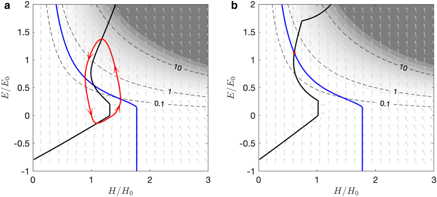
Fig. 9. The effect of including crevasse-activated surface meltwater routing, with default parameter values shown in Table 1, $\hat{T}_{\rm a} = -0.8$ , $\hat{a} = 0.3$
 , u 1 = 0 and u 2 – 100 m a−1. (a) No surface meltwater input, exhibiting an unstable steady state. (b) The same input parameters as (a) but with the β(u) function activated, exhibiting a stable steady state. In this case, crevasses are opened by sliding, allowing larger water inputs to the bed, which sustain rapid sliding. The noticeable kink near the top of the E-nullcline (black line) corresponds to where u = u 2. Background shading indicates the ice speed u.
Second, for other combinations of input parameters, glaciers continue to have oscillatory steady states when the β(u) function is activated, but with changes in the characteristics of the surge cycle. The case shown in Figure 10 uses the same parameter values as in Figure 9, except for the value for accumulation. In the previous case, the introduction of crevassing stabilizes the glacier, whereas in this case the glacier remains in a surging state but with a higher peak velocity and a shorter period. The effect of activating the β(u) function is shown in Figure 10 (m–x). As the ice velocity begins to increase during late quiescence (due to velocity–frictional heating feedback), increasing surface water inputs trigger rapid flow acceleration. A fast velocity-crevassing feedback then allows the glacier to bypass the slower velocity-heating feedback, leading to more rapid surge onset.
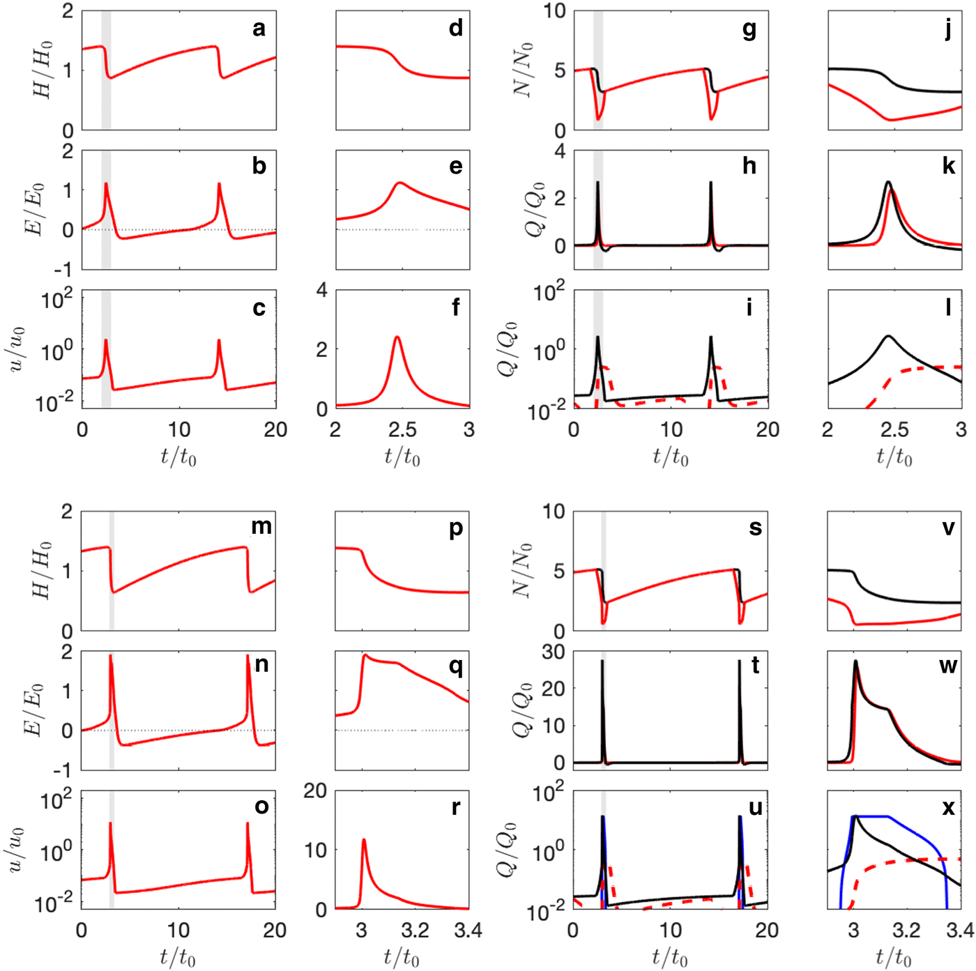
Fig. 10. Example solutions exhibiting oscillatory behaviour with the β(u) function off (a–l), and on (m–x). Same input parameter values as in Figure 9, but with $\hat{a} = 0.3,$ u 1 = 10 m a−1 and u 2 = 100 m a−1. Panels d–f, j–l, p–r and v–x show detail in the grey-shaded zones in panels a–c, g–i, m–o and s–u, respectively. Panels g–l and s–x show the effective pressure N (with ice pressure in black, which provides a cap on N); enthalpy fluxes Q (black is the sum of all heat sources minus conductive cooling, red is subglacial discharge); and a breakdown of heat sources (black is frictional heating, red is geothermal minus conductive cooling and is negative when shown dashed, blue is surface water penetration). Note different scales in some cases (the fluxes are larger when surface water is included).
The length of the surge cycle is sensitive to the choice of u 1 and u 2, the velocity bounds where surface water inputs begin and saturate, respectively. Setting u 1 to zero shortens the cycle because faster sliding is permitted throughout. Conversely, increasing u 1 lengthens the cycle, because the glacier can have long periods of zero surface water input and very low velocity during quiescence. These results partly reflect the heuristic way that we have implemented surface water inputs in the model, but they hint that the length of the surge cycle is affected by several factors, not simply accumulation rates.
Taken across the whole climatic parameter space, activation of the β(u) function reduces the size of the envelope associated with dynamic oscillations, removing a region from the warm–humid end of the surging regime (Fig. 11). That is, surface-to-bed drainage allows some formerly ‘surge-type’ glaciers to attain stable steady states, in which constant flow speeds are sustained by surface melt rather than basally generated water alone. Recall that channelized drainage does not feature in this version of the model, so this interpretation applies to the case where high water fluxes are associated with high water storage in a distributed drainage system. As was the case in the simplest form of the model, changes in glacier length and bed slope shift the position of the surge regime. Thus, for a population of glaciers with varying length and slope, the model predicts that surge-type and non-surge-type glaciers coexist in certain climatic regimes.
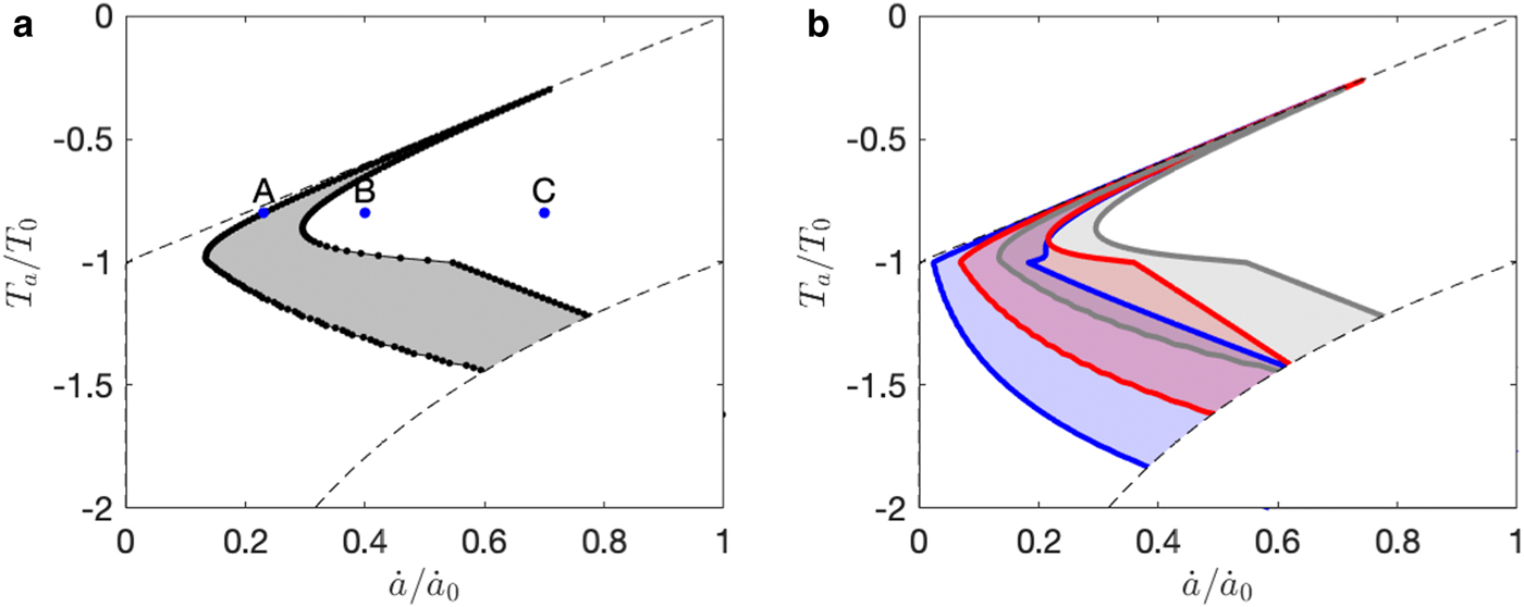
Fig. 11. (a): Surging regime for the default parameters with the β(u) function activated, allowing surface meltwater to penetrate to the bed via crevasses. (b): Surging regime for default parameters (grey), double the length (pink) and half the slope (blue), with the β(u) function activated.
The diagonal spike at the warm end of the surge regime in Figure 11 deserves comment. This spike represents environments where accumulation is only slightly larger than net melt, and balance velocities are thus very low. In the model, stable, steady-state solutions do not exist for glaciers in this region, because their balance velocities are inconsistent with their basal water (enthalpy) balance, irrespective of whether water is supplied from basal melt alone or basal melt plus surface water inputs. This spike in the surging regime may be an artefact of the lumped model formulation, which neglects spatial variations in accumulation and melt over the glacier surface. However, it raises the possibility that small glaciers close to the limit of viability may be prone to dynamic instabilities.
5.3 Two-component drainage system, with surface water input
The model runs using the two-component drainage model (13) exhibit changes in drainage system configuration over the course of surge cycles, which in turn influence the dynamics. An example is shown in Figure 12, in which the glacier is warm-based throughout. During the quiescent phase, R-channels are essentially absent (S is very small), and enthalpy (in the form of water) gradually builds up in the distributed drainage system in response to the geothermal heat flux. Ice velocities are very low, and surface accumulation causes an almost linear increase in ice thickness. In late quiescence, increasing enthalpy in the distributed system leads to increasing ice flow velocities, and frictional heating becomes a significant enthalpy source. Higher ice velocities increase surface water input, further increasing basal enthalpy and ice flow velocities. As basal water storage increases, falling effective pressure N allows channel radius S to increase (15), and R-channels rapidly grow at the expense of the distributed system, discharging stored water and terminating the surge. Increasing N causes channel shrinkage, and the glacier bed reverts to a low-enthalpy distributed system.

Fig. 12. An example solution of a run with the β(u) function activated and the two-component drainage model, showing variations in H, E, u, S, N and Q. On the Q plot, the red line shows the total water discharge (distributed and channelized) and the black line shows the combination of all water inputs (geothermal and frictional melting, surface-to-bed drainage, minus conductive cooling). The second and fourth columns show the inset regions in more detail.
This model run represents a temperate glacier surge involving switches in the basal drainage system. However, the hydrologic switch works in a subtly different way to previous formulations, which invoked a spontaneous transition from a channelized to a distributed drainage system as a trigger for surge onset, in addition to the reverse transition for surge termination (e.g. Fowler, Reference Fowler1987a). In our model, the glacier has a low-enthalpy distributed drainage system during quiescence, which gradually transitions to a high-enthalpy distributed system during late quiescence and surge. Surge termination occurs due to switching to a channelized system, allowing rapid discharge of stored water. The opposing switch, however, simply occurs when the bed runs out of water, channels collapse and drainage reverts to a low-enthalpy distributed system.
In the present implementation of the model, solutions with steady-state channelized drainage systems were not found. Where surface water supply is large, the two-component drainage model produces a set of almost stable steady states with respect to mass, but with oscillations in channel size and basal water storage (Fig. 13). These oscillations do not significantly affect frictional heating or dynamics; ice thickness is essentially constant and velocity remains small. They are thus quite different from surge cycles, but reflect instabilities in the modelled drainage system rather than the glacier dynamics.
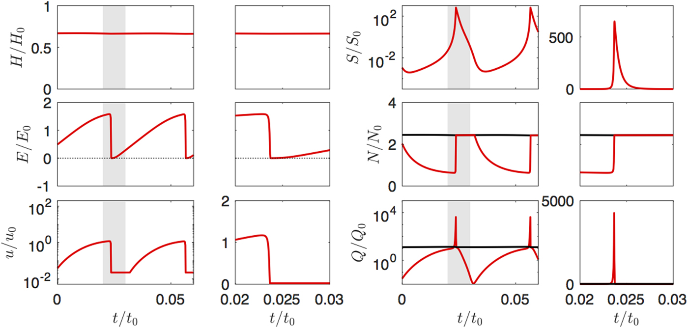
Fig. 13. Example output from the two-component drainage model, using the same parameters as in Figure 10, but with u 2 = 0 (i.e. all surface melt always penetrates to the bed. This displays rapid oscillations of channel size and basal water storage, but ice thickness is almost constant and velocity remains small. Cycle period (~5 years in the example shown) varies with the choice of input parameters and is of no particular significance.
6. Summary and discussion
6.1 Predictions of enthalpy balance theory
The model results can be summarized as a set of hypotheses that can be tested against existing or future observations. For the simplest implementation of the model (single-component drainage system and no surface-to-bed drainage), enthalpy balance theory predicts:
(1) Non-surge-type or ‘normal’ glaciers have stable steady states with respect to their mass and enthalpy budgets. In terms of E–H phase portraits, the nullcline intersections are point attractors and lie on the upper or lower branches of the E-nullcline (Fig. 3).
(2) Surge-type glaciers have unstable steady states with respect to their mass and enthalpy budgets. These steady states are unstable to small perturbations, which set in train feedbacks between enthalpy balance and dynamics, which in turn lead to periodic mass, enthalpy and velocity cycles. In phase portraits, solutions follow limit cycles, orbiting around nullcline intersections that lie on the middle branch of the E-nullcline.
(3) Climate, glacier geometry and bed properties determine whether glaciers have stable or unstable steady states.
(4) In cold, dry climates, glaciers have low balance fluxes and are low-enthalpy producers; enthalpy production can be balanced by conductive heat losses due to low mean annual air temperatures, particularly where ice is thin.
(5) In warm, humid climates, glaciers have high balance fluxes and are high-enthalpy producers. High enthalpy at the bed allows enthalpy production to be offset by high subglacial water discharge. In the single-component model, high discharge occurs when water storage w is high (12).
(6) In intermediate climates, neither conduction nor water discharge can evacuate enthalpy at steady rates that match the production from geothermal heat flux plus frictional heating (expenditure of potential energy). The resulting steady-state conditions are unstable, and ice thickness, enthalpy and velocity undergo periodic oscillations.
(7) The model predicts the following sequence of processes over the course of surge cycles. During quiescence, velocities are less than balance velocities, and mass accumulates. Enthalpy at the bed is low at the start of the quiescent period, and gradually increases because geothermal heating exceeds enthalpy losses. Once enthalpy rises high enough to initiate sliding, feedback between frictional heating and sliding speed causes rapid flow acceleration and transition to the surge phase. The surge terminates when basal water is lost faster than it is produced. Depending on the environmental conditions, the glacier bed may remain entirely temperate during the surge cycle, or enter a cold-based condition during quiescence. In both cases, the physical processes underlying the surge cycle are essentially the same.
(8) Glacier length and slope influence the distribution of unstable states with respect to accumulation and mean annual air temperature. In our model, length affects dynamics through its impact on the balance flux and subglacial discharge, and slope affects dynamics through its impact on the hydraulic gradient and basal shear stress. In cold, dry climates, long, gently sloping glaciers are more likely to be surge-type than short, steep glaciers.
(9) Basal hydraulic conductivity influences the distribution of surging glaciers by altering drainage system efficiency (strictly, this statement applies to our hydraulic conductivity parameter $\tilde{K}$
 , which has different units to hydraulic conductivity as normally defined; here we use ‘hydraulic conductivity’ for brevity, with this caveat). Low hydraulic conductivity (inefficient drainage) encourages surging behaviour in warm, humid climates, whereas high conductivity (efficient drainage) encourages stable steady states. Variations in length, slope and hydraulic conductivity in a population of glaciers mean that the distribution of surge-type glaciers and non-surge-type glaciers will overlap.
(10) Climate change can alter the geographical distribution of surge-type glaciers.

When surface water is allowed to access the bed via crevasses as flow speeds increase, additional behaviour emerges:
(11) Surface water input can influence surge phase dynamics by increasing basal enthalpy and ice velocities more rapidly than is possible by velocity-heating feedbacks alone. The influence on quiescent phase duration is complex, however, and the surge cycle may be shortened or lengthened depending on input parameters.
(12) Inputs of surface water eliminate unstable steady states in part of the warm–humid end of the climate envelope. Where surface-to-bed drainage occurs, stable flow speeds can be maintained by surface meltwater inputs rather than through frictional heating alone. This statement applies for the single-component drainage model, where high water throughput corresponds to high basal water storage.
Finally, the addition of a two-component drainage system with both distributed and channelized elements allows hydraulic switching to influence the dynamics:
(13) Switching between distributed and channelized modes of the drainage system can occur over the course of surge cycles. A low-enthalpy distributed system exists during quiescence, which gradually transitions to a high-enthalpy distributed system during late quiescence and the surge phase. When the effective pressure N becomes very low, reduced creep closure allows rapid development of an efficient channel system, terminating the surge. Thus, hydrologic switching (from a distributed to a channelized system) triggers surge termination, and the opposing switch (channels to a distributed system) occurs when the bed runs out of water. The switch to a distributed drainage system does not trigger a surge, but sets up the initial conditions necessary for the build-up of mass and enthalpy during quiescence.
(14) It is possible that stable steady states exist with low water storage and high throughput, with efficient R-channels maintained by surface-to-bed drainage. In the present model, these high-throughput states have almost constant ice thickness and low-velocity throughout, but the subglacial channel undergoes spontaneous oscillations in size.
6.2 Comparison with observations
Some of the hypotheses listed above can be tested with existing data, while others will require new, targeted observations before rigorous testing is possible.
Predictions of the theory are consistent with global-scale data on the distribution of surge-type glaciers with respect to mean annual precipitation and air temperature (Sevestre and Benn, Reference Sevestre and Benn2015; Figs 1, 6, 8). Importantly, we have made no attempt to tune model parameters to optimize the match between model results and observations; such an attempt would have little value given the idealized, lumped model geometry, the approximate nature of key equations, and the indicative character of the ERA-I climatic data. Given this lack of tuning, the similarity between model predictions and observations is striking, particularly the concentration of surge-type glaciers in climates intermediate between cold–dry and warm–humid environments, and the overlapping distributions of surge-type and non-surge-type glaciers with different geometries.
The model results are consistent with the observed relationships between glacier geometry and surging behaviour, and indicate that length and slope are distinct influences and not simply two perspectives on a single dependency (cf. Clarke, Reference Clarke1991). Notably, the model correctly predicts that in cold, dry environments (i.e. Arctic Canada: Fig. 1), only long, low-gradient glaciers will be of surge type. In the model, short glaciers in dry climates have low balance fluxes and are low-enthalpy producers; steeper glaciers are thin and lose enthalpy efficiently by conduction to the cold atmosphere. New observations are needed to further test this model prediction.
In the model, low hydraulic conductivity encourages surging behaviour because it reduces the ability of the subglacial drainage system to evacuate enthalpy from the bed. This result offers an explanation for the observed association between surge-type glaciers and weak sedimentary rocks (e.g. Jiskoot and others, Reference Jiskoot, Murray and Boyle2000). Glaciers eroding weak lithologies (e.g. shales) tend to produce thick, fine-grained tills with lower hydraulic conductivity, likely to impede water flow at the bed (Clark and Walder, Reference Clark and Walder1994). However, substrate type likely influences glacier dynamics in complex ways, and detailed observations are required to further illuminate the relationships between enthalpy balance and substrate type.
Surge cycle lengths are very long (hundreds of years) in the examples illustrated in Figures 4, 10, 12, reflecting the low net accumulation prescribed in these cases. Examples with higher accumulation (not shown) exhibit shorter cycle lengths (decades), consistent with the idea that accumulation is a key control on quiescent phase duration (e.g. Dowdeswell and others, Reference Dowdeswell, Hodgkins, Nuttall, Hagen and Hamilton1995; Eisen and others, Reference Eisen, Harrison and Raymond2001). However, cycle length must also reflect the amount of ice drawn down during the surge phase, which determines the total amount of build-up that must occur before the next surge is initiated. Surge-phase draw-down is a function of ice velocity and surge duration, which in turn reflect a complex web of dynamic and hydrological processes. Closer correspondence between modelled and observed surge periods could be achieved by tuning several possible combinations of the parameters governing relationships between stress, effective pressure, ice velocity, surface-to-bed drainage, water storage and subglacial discharge (e.g. R, p, q, $\tilde{C}$ , α, β, u 1 and u 2 in Eqns (7), (10), (12), (13) and (16)). We have not attempted this, because any parameter combination choice would be arbitrary and the exercise would not yield additional insights into how these processes interact to control cycle length in real-world cases. Careful work with fully spatial models will be needed to disentangle the roles of dynamic and hydrological processes in controlling surge cycle length.
Our model runs focus on glaciers under constant climate conditions, but the predicted climate dependence of surging implies that the spatial distribution of surge-type glaciers could shift in response to climate change. This is consistent with evidence from Svalbard, where many small glaciers are known or inferred to have surged during the Little Ice Age, but now have strongly negative mass balance and can no longer build up the necessary mass to maintain the surge cycle (James and others, Reference James2012; Sevestre and others, Reference Sevestre and Benn2015). Indeed, it may be said that these glaciers are no longer in quiescence, but a climatically induced senescence. In terms of the climatic parameter space shown in Figure 6, this is equivalent to moving a glacier from the surge regime into the region of glacier unviability in the top left of the diagram. A similar regime change may have affected glaciers in the Pyrenees that appear to have been surge-type during the Little Ice Age (Cañadas and Moreno, Reference Cañadas and Moreno2018). In the Austrian Alps, Vernagtferner repeatedly surged during the Little Ice Age, but ceased to do so in the warmer climate of the 20th century (Hoinkes, Reference Hoinkes1969; Kruss and Smith, Reference Kruss and Smith1982). Evidence from lake sediments indicates that a change in the opposite direction affected Eyjabakkajökull in Iceland, which switched from non-surge type to surge type ~2200 years ago (Striberger and others, Reference Striberger2011).
Several studies have attributed changes in surge magnitude and frequency to climate change. For example, Frappé and Clarke (Reference Frappé and Clarke2007) showed that the ‘slow’ 1980–2000 surge of Trapridge Glacier lacked the fast flow phase that occurred during the previous surge in the 1940s, probably due to diminished mass build-up. In contrast, Copland and others (Reference Copland2011) argued that recent temporal clustering of surges in the Karakoram occurred because surge cycle length has been shortened by an increase in precipitation. Dunse and others (Reference Dunse2015) proposed that a major surge of the Basin 3 outlet glacier of Austfonna, Svalbard, was triggered by increased amounts of surface meltwater penetrating crevasses and thawing formerly cold ice. Less convincingly, Nuth and others (Reference Nuth2019) suggested that some recent surges in Svalbard were triggered by near-margin thinning and freezing. In all these cases, climatic factors appear to have influenced the timing and/or magnitude of surges, rather than initiated surging behaviour in hitherto non-surge-type glaciers. As such, these cases are qualitatively different from the climatically driven regime changes implied by the current suite of model runs. Implications of enthalpy balance theory for understanding glacier dynamic response to transient climatic states is the focus of ongoing work.
Enthalpy balance theory makes the important prediction that polythermal and temperate glacier surges occur by essentially the same mechanism. In both cases, an excess of enthalpy gains relative to losses results in the accumulation of water in a distributed drainage system. In polythermal glaciers, the bed may undergo an intermediate cycle of freezing and thawing during quiescence, although it should be noted that larger polythermal glaciers may remain largely warm-based throughout the surge cycle (Sevestre and others, Reference Sevestre and Benn2015). The prediction that polythermal and temperate glacier surges have a common dynamical basis is consistent with population-scale data on the distribution of surge-type glaciers, and the observation by Frappé and Clarke (Reference Frappé and Clarke2007) that thermal regime is ‘collateral to the surging phenomena rather than essential’. At the individual glacier scale, detailed mass and enthalpy budget analysis of the polythermal glacier Morsnevbreen, Svalbard, has shown that enthalpy sources and sinks underwent the predicted sequence of changes over the course of its most recent surge cycle (Benn and others, Reference Benn2019). Comparative analyses will be conducted for temperate surge-type glaciers to further test the theory.
The theory also predicts that temperate glacier surges can occur in the absence of switches in drainage system configuration. Introduction of a two-component drainage system affects some of the details of surge evolution, but not the underlying relationships between mass and enthalpy budgets for glaciers with unstable steady states. Importantly, and in contrast with previous models of hydrologic switching (e.g. Jay-Allemand and others, Reference Jay-Allemand, Gillet-Chaulet, Gagliardini and Nodet2011; Mayer and others, Reference Mayer, Fowler, Lambrecht and Scharrer2011), in our model, a transition from R-channels to a distributed system does not act as a surge trigger. Rather, a channel-to-distributed transition occurs after surge termination when basal water storage is drawn down, and simply resets the system in a low-storage state at the start of quiescence. This offers a solution to a long-standing difficulty with hydrological switch theory, namely, exactly what mechanisms could trigger a switch from channelized drainage to a high-storage distributed system, and why this should occur on some glaciers but not others (Harrison and Post, Reference Harrison and Post2003). Moreover, it is important not to view distributed and channelized drainage systems in terms of a simple binary switch. Both drainage types can exist simultaneously on different parts of the same glacier, and in principle water could accumulate in a distributed system under some parts of a glacier system while other parts continue to be drained by surface-fed conduits (Fischer and Clarke, Reference Fischer and Clarke2001; Benn and others, Reference Benn, Kristensen and Gulley2009; Schoof and others, Reference Schoof, Rada, Wilson, Flowers and Haseloff2014). If a surge is initiated, conduits could then be destroyed following surge propagation, in which case a switch from channelized to distributed drainage would be a consequence rather than the cause of a surge. The difficulty of determining drainage system configurations means that testing hydrological aspects of surge theory presents major challenges.
In all cases, our model predicts abrupt termination of surges due to the discharge of water from the bed, either via a high-storage distributed system (‘blister flux’) or a switch to an efficient channelized system. This is consistent with the previous work on the hydrology of surge-type glaciers that has shown that abrupt surge terminations are triggered by step changes in drainage efficiency (e.g. Kamb and others, Reference Kamb1985; Kamb, Reference Kamb1987). Not all surges terminate abruptly, however, and some instead undergo gradual slowdowns spread over multiple seasons (e.g. Luckman and others, Reference Luckman, Murray and Strozzi2002; Sund and others, Reference Sund, Lauknes and Eiken2014; Sevestre and others, Reference Sevestre2018; Benn and others, Reference Benn2019). Gradual slowdowns are typical of polythermal glaciers in Svalbard (though not all, see Kristensen and Benn, Reference Kristensen and Benn2012), and may reflect the removal of hydraulic barriers during surge-front advance rather than a drainage system switch. Simulation of these effects will require a spatial treatment of basal hydrology.
For combinations of input parameter values that allow a large volume of surface meltwater to access the bed, the model predicts almost stable steady states with respect to mass and velocity but with oscillations of channel size and basal water storage. Stable steady states with respect to both mass and water storage were not found with the present model. This reflects the simplified representation of hydrology in the lumped model, particularly the assumptions that the effective pressure in the channel and distributed system are the same, and that the hydraulic gradient is constant and determined by the bed slope. Indeed, a slightly modified version of the present model (not shown) can allow for the possibility of stable channels at high discharge. On real glaciers, surface meltwater production (and hence surface-to-bed drainage) fluctuates on diurnal, seasonal and intermediate timescales, so examples of such steady states are unlikely to occur in nature. It is also notable that spontaneous subglacial water pressure oscillations unrelated to water supply variations have been observed (Schoof and others, Reference Schoof, Rada, Wilson, Flowers and Haseloff2014), and modelling indicates that these are due to conduit growth and decay cycles analogous to the jökulhlaup instabilities described by Nye (Reference Nye1976). This raises the possibility that unforced drainage system oscillations can occur across a wide range of timescales, with a corresponding range of impacts on ice dynamics. This may account for some short-term dynamic instabilities such as ‘mini-surges’ and pulses (e.g. Humphrey and others, Reference Humphrey, Raymond and Harrison1986; Kamb and Engelhardt, Reference Kamb and Engelhardt1987; Turrin and others, Reference Turrin, Forster, Sauber, Hall and Bruhn2014; Herreid and Truffer, Reference Herreid and Truffer2016).
Our model experiments do not include seasonal cycles, but the predicted impact of surface water input is consistent with the observed timing and location of rapid speed-up events during surges. In Svalbard, several studies have shown that expansion of crevasse fields during the early stages of surges has created templates for areas of flow acceleration at ablation season onset (Dunse and others, Reference Dunse2015; Sevestre and others, Reference Sevestre2018; Gong and others, Reference Gong2018; Benn and others, Reference Benn2019). The role of surface-to-bed drainage in stabilizing the flow is illustrated by Kronebreen, a perennially fast-flowing tidewater glacier in the midst of the Svalbard surge cluster. Convergent flow on the upper glacier focuses accumulation from a large catchment area, giving Kronebreen a higher balance flux than its neighbours. The effect of convergent flow is equivalent to shifting the glacier into a higher-precipitation environment than the adjacent glaciers. High velocities are maintained by water reaching the bed via the intensely crevassed glacier surface (How and others, Reference How2017; Vallot and others, Reference Vallot2017).
6.3 Model formulation: limitations and future prospects
In keeping with our aim of exploring fundamental principles underlying glacier dynamics, we have adopted a lumped model approach incorporating simple equations to represent system components. Inevitably, this approach glosses over much fine detail, and representations of processes such as conduction of heat, basal sliding and hydrology are necessarily approximate. The model results, however, are robust for plausible values of most input parameters. Model sensitivity is greatest for the exponent α in the drainage law (12). To achieve the stable upper branch of the E-nullcline, α must be larger than 1/p (the exponent in the sliding-law: Eqn (8)). In physical terms, this means that for stable steady states to occur under warm, humid conditions, drainage must be efficient enough to cope with the energetic consequences of faster ice flow (i.e. frictional heating). Since non-surge-type glaciers are common in relatively warm, humid environments, this feature of the model likely reflects an important principle, although of course only in an approximate, generalized way.
The present implementation of the model does not allow free evolution of the ice-surface slope and omits the pressure term in the hydraulic potential gradient. These approximations likely limit the range of behaviour exhibited by the model, but were unavoidable because of its non-spatial character. More sophisticated treatment of these system components will require a fully spatial model, either in 2-D (flowline) or 3-D. This will allow particular processes and geometries to be examined in more detail, but at the expense of generality.
The present lumped model is based on the assumption that surge initiation occurs in a reservoir zone where accumulation exceeds net ablation, whereas some surges initiate in glacier ablation zones (e.g. Björnsson and others, Reference Björnsson, Pálsson, Sigurđsson and Flowers2003; Dowdeswell and Benham, Reference Dowdeswell and Benham2003; Murray and others, Reference Murray2012; Sevestre and others, Reference Sevestre and Benn2015; Abe and others, Reference Abe, Furuya and Sakakibara2016). Potentially, this type of surge behaviour could be accommodated in the model by allowing ice inflow (i.e. modifying the flux divergence term in Eqn (2)), thus permitting thickening to occur even if the surface mass balance is negative. This possibility will be explored in future work.
Many important phenomena associated with glacier surges are inherently spatial. It is widely accepted that spatial variations in basal thermal regime strongly influence the trajectories of polythermal glacier surges (e.g. Clarke and others, Reference Clarke, Collins and Thompson1984; Fowler and others, Reference Fowler, Murray and Ng2001; Murray and Porter, Reference Murray and Porter2001). For example, cold-based ice near glacier termini may impede water discharge and exacerbate instabilities associated with basal water accumulation in warm-bedded regions up-glacier. Similarly, spatial variations in basal drainage systems (including the location of water sources and sinks) likely play a key role in surge propagation (e.g. Jay-Allemand and others, Reference Jay-Allemand, Gillet-Chaulet, Gagliardini and Nodet2011; Sevestre and others, Reference Sevestre2018). Spatial phenomena can be considered in terms of enthalpy gradients, and the advection of enthalpy between sources and sinks. A fully spatial development of enthalpy balance theory has the potential to shed light on individual cases of surge initiation and propagation, and to explore the ways that local conditions manifest general principles. For further discussion of ways in which spatial phenomena can modulate enthalpy and mass fluxes, see Benn and others (Reference Benn2019).
7. Concluding remarks
Enthalpy balance theory draws together several elements of previous models, and offers to explain the full spectrum of glacier dynamic behaviour within a single coherent framework. It shows that polythermal and temperate glacier surges can be explained by a single, general theory – not two, or many. Perhaps more importantly, it also offers an explanation of why the majority of glaciers do not surge. By design, our implementation of the theory takes a non-spatial, lumped approach, appropriate for a population-scale investigation of the fundamental principles underlying glacier dynamics. Implementation of the theory in two or three dimensions will allow more detailed exploration of key processes at the individual glacier scale.
In this paper, we have emphasized unifying principles underlying glacier dynamics, but of course the diversity of surge phenomena also requires attention. As a more detailed and comprehensive picture of glacier dynamics emerges, it is becoming clear that glaciers exhibit a very wide range of forced and unforced oscillatory behaviour across a wide range of timescales, and the distinction between surge-type and non-surge-type glaciers appears less distinct than it once did (Herreid and Truffer, Reference Herreid and Truffer2016). Enthalpy balance theory provides a unique viewpoint from which to explore this diversity.
Acknowledgements
Funding for DIB was provided by NE/R018243/1 REBUS (Resolving Enthalpy Budget to Understand Surging).
Appendix: Non-dimensionalized model
We cast the model in non-dimensional form by scaling each of the variables with suitable values, denoted with subscript 0. These scales are chosen according to certain balances in the equations. We take representative values for a 0, l 0 and θ 0, and then define

(In practice, we choose the values of R, C and K in order to attain expected typical values of u 0, N 0 and E 0.) Typical values for the parameters used, and the resulting scales, are shown in Table 1.
After scaling all of the variables, and putting together the different ingredients, the non-dimensional model can be written as three coupled ordinary differential equations:


where

and where $\hat{a} = a/a_0$ is the dimensionless accumulation rate, $\hat{m} = {\rm DDF}\lpar {T_{\rm a}-T_{{\rm offset}}} \rpar /a_0$
 is the dimensionless melt rate, $\hat{T}_{\rm a} = T_{\rm a}/T_0$
 is the dimensionless air temperature, $\hat{\Theta} = \sin \theta /\sin \theta _0$
 is the normalized slope, and $\hat{l} = l/l_0$
 is the dimensionless length. ${\hat{a},\;} \; \hat{l}\; {\rm and}\; {\hat{\rm \Theta}}$
 could all be chosen to be 1 by the choice of the relevant scale, but are retained in the equations because they are primary climatic and geometric parameters whose influences we explore.
There are a number of other dimensionless parameters, defined by

These represent the importance of geothermal heating, conductive cooling, and surface meltwater heating, relative to frictional heating (λ, κ and δ), the ratio of the timescale for enthalpy changes compared with ice thickness changes (μ), the ratio of typical effective pressure to ice pressure (χ), the relative importance of internal deformation to sliding (λ), the timescale for channel growth relative to ice-thickness changes (ν), the importance of dissipative heating compared to creep closure (σ) and the dimensionless incipient channel opening rate ($\widehat{{\dot{S}}}_0$ ).
).
The single-component drainage model is obtained simply by setting S = 0 and ignoring the S evolution equation, so there are just two autonomous ordinary differential equations for H and E. The behaviour of the system can be investigated using standard methods of phase-plane analysis. We locate steady states as the intersections of the nullclines (where both time derivatives are zero) and then perform a linear stability calculation around such states to determine whether they are stable or unstable. We identify a parameter regime as having surging solutions if the only steady state is unstable. The solutions in such cases lock on to periodic orbits in the phase plane, which correspond to the surge cycle. The generic shape of the nullclines is as described in the main text, and surging states correspond roughly (though not exactly) to when the intersection of the nullclines lies on the central branch of the E-nullcline.


 Open access