


Introduction
Numerical modeling of glaciers is motivated by two main difficulties inherent in glacier research: we have few data and the equations arc difficult to solve. Data arc sparse because glaciers lend to he in inaccessible places with inhospitable climates, they move too slowly or are too broken by crevasses for easy measurements and the most interesting processes occur at the bed, which is even less accessible. The equations that describe the creep of ice are made difficult by the nonlinear theology, usually represented by the Reference GlenGlen (1955) flow law that is commonly accepted as the best available approximation for a constitutive relation. A good numerical model can aid in interpreting the expensive, sparsely distributed data. Computers can also turn the complex equations of motion into a multitude of simple equations, replacing analytical elegance with a great capacity for repetition but nevertheless getting a result where otherwise there would be none. With these needs, modeling has proceeded in a hierarchical fashion, with models of various dimension and various levels of simplification developed within the limitations of computer capabilities and the needs of particular investigators. (The hierarchical structure of modeling efforts was noted and reviewed by Reference Hutter, Yakowitz and SzidarovszkyHutter and others (1986).)
One can decrease computational requirements geometrically by reducing the dimension of a numerical model. For a glacier with a substantial symmetry to exploit or when data are restricted to a simple plane or line, models of reduced dimensionality, such as flow-plane models, flowline models or vertical-column models, may be the most justifiable. Similarly, large ice-sheet models may exploit the smallness of longitudinal stresses to parameterize the vertical dimension. The pioneering three-dimensional model of Reference JenssenJenssen (1977) and recent efforts by Reference HerterichHerterich (1988) and Reference HuybrechtsHuybrechts (1990a, Reference Huybrechtsb) use that simplification in simulating the entire Antarctic ice sheet. Most small valley glaciers lack symmetries and have large longitudinal stresses. Large ice sheets may lack symmetries in such interesting areas as the accumulation zone of an ice stream. It therefore makes sense to develop some models without intrinsic dimensional simplifications.
A fully three-dimensional model will be used here to explore the dynamics of Storglaciären. The glacier exhibits intrinsically three-dimensional How patterns with no reasonable symmetries and its center-line flow has a complexity that cannot be readily removed via the use of shape factors. The purpose is both to demonstrate the capabilities of the model and to elucidate the driving stresses and resistances that give Storglaciären its dynamics.
Model Description
This model is a fully three-dimensional generalization of the (low-plane model described by Reference HansonHanson (1990). That How-plane model solved equations for conservation of mass, momentum and thermal energy in a vertical flowplane, with both steady-state and time-stepping capabilities. That model has been fully extended to three dimensions but only the dynamics part is used in this paper. Basic equations are the Stokes equations for steady conservation of momentum and conservation of mass for an incompressible medium, expressed here as

and
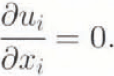
Here, ![]() is the deviatoric stress tensor, p is pressure, gi
is the gravity vector, ui
is velocity and xi
is the position vector. The Einstein convention of summing on repeated indices over their range is used throughout this paper. The indices in Equations (1)– (3) range through the three spatial dimensions of the model. The model specifics that x3
points vertically upward, while xi
and x2
are horizontal coordinates such that the three coordinates form a right handed orthogonal coordinate system. Later discussion will treat the (x1, x2, x3
) system as an (x, y, z) system, for convenience.
is the deviatoric stress tensor, p is pressure, gi
is the gravity vector, ui
is velocity and xi
is the position vector. The Einstein convention of summing on repeated indices over their range is used throughout this paper. The indices in Equations (1)– (3) range through the three spatial dimensions of the model. The model specifics that x3
points vertically upward, while xi
and x2
are horizontal coordinates such that the three coordinates form a right handed orthogonal coordinate system. Later discussion will treat the (x1, x2, x3
) system as an (x, y, z) system, for convenience.
Solution of Equation (1) for velocity requires a constitutive relation. The effective viscosity, μ, is defined such that
where ![]() is the strain-rate tensor. The viscosity is calculated from
is the strain-rate tensor. The viscosity is calculated from
where n is a constant, taken here to be 3, ![]() is the square root of the second invariant of
is the square root of the second invariant of 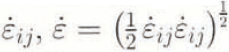 and Β is a stiffness parameter whose value depends on the temperature, crystal fabric and water content of the ice. Equations (3) and (4) taken together are the familiar Reference GlenGlen (1955) power law for flow.
Numerical solution of the model requires the discretization of the domain into generalized eight-node “bricks”, which arc three-dimensional generalizations of the Taig quadrilateral, a linear, isoparametric element (Reference Irons and AhmadIrons and Ahmad, 1980). The elements approximate hexahedra but the four nodes that define each of the six faces need not be coplanar.
The model domain is broken into M elements defined by Ν nodes and the fundamental equations are solved in two different ways. Momentum equations are constructed from Equation (1) using Galerkin’s method, with second derivatives removed using Green’s theorem. Model velocities thus consist of nodal values ![]() that are interpolatable to a piecewise continuous (C0) function. Modeled pressures take on constant values within each clement. Equations for conservation of mass are produced via direct integration of Equation (2) over each element. All integrals over elements are evaluated using two-point Gauss Legendre quadrature in each dimension. The equations then produced have the appearance of a set of linear equations of order 3Ν + M. However, the coefficients contain the viscosity μ which further includes velocities within its definition, so the equations must be solved iteratively.
that are interpolatable to a piecewise continuous (C0) function. Modeled pressures take on constant values within each clement. Equations for conservation of mass are produced via direct integration of Equation (2) over each element. All integrals over elements are evaluated using two-point Gauss Legendre quadrature in each dimension. The equations then produced have the appearance of a set of linear equations of order 3Ν + M. However, the coefficients contain the viscosity μ which further includes velocities within its definition, so the equations must be solved iteratively.
Boundary conditions may include applied stresses or fixed velocities. The upper surface is normally left as a free surface, with no stress applied. Equations produced will be underdetermined unless some velocity boundary conditions an-applied, fixing velocities of zero for points frozen to the bed or sidewall satisfies the condition. Basal velocities at unfrozen nodes are more problematic. One may specify a sliding velocity, which requires a sliding law. One may specify a three-dimensional stress, which requires complete knowledge of the stress field. One may specify a resistive stress and constrain the direction of flow to follow the base, which requires a knowledge of at least the stress-coupling between ice and bed. Simulations here will use a sliding law to specify speeds at all unfrozen basal nodes, with limitations of that approach to be discussed below.
As with the two-dimensional version of this model dealt with by Reference HansonHanson (1990), the model has been tested against the theoretical solution of Reference NyeNye (1957) for a slab of homogeneous ice of uniform thickness on an infinite plane slope. Iterative solution of the model stops when the largest velocity change between iterations is smaller than an arbitrarily specified convergence criterion, which was 10−4 m year−1 in these simulations. Model simulations successfully reproduce Nye’s solution to within a digit of the convergence criterion.
Storglaciären Simulations
Model Domain and Tuning
Storglaciären is a small, temperate valley glacier in the Kebnekaise Massif of northern Sweden. It is most widely known for having a record of mass-balance measurements dating back to the 1940s (Reference HolmlundHolmlund, 1987). Extensive measurements of velocity have also been made on this glacier, including long-term surface velocities, borehole deformations and short-term velocity variations (Reference Hooke, Calla, Holmlund, Nilsson and StroevenHooke and others, 1989, Reference Hooke, Pohjola, Janssen and Kohier1992; Reference Jansson and HookeJansson and Hooke, 1989; Reference Hanson and HookeHanson and Hooke, 1994). These data, combined with available detailed surface maps produced photogrammetrically and bottom topography from radio-echo sounding (Reference HolmlundHolmlund and Schytt, 1987; Reference ErikssonEriksson, 1990), provide the necessary background information for model simulations.
A model domain was established for Storglaciären consisting of 5643 nodes surrounding 4626 elements (Fig. 1). The elements were arranged in 257 vertical columns of 18 elements. Through most of the glacier, basal elements are 3 m thick and element thicknesses increase linearly with height to provide the required total glacier thickness. In areas less than 54 m thick, elements are of equal vertical thickness, with a minimum total column thickness of 5 m. The horizontal pattern of nodes was developed by hand, based on the criteria of minimizing the number of nodes needed while putting greater node densities where the horizontal stress gradients were expected to be higher.

Fig. 1. Model element grids and coordinates for Storglaciären simulations, a. Horizontal grid with x (east) and y (north) coordinates. Circles connected with the dotted line indicate the chain of nodes used as an approximate central flowline for cross-section diagrams. Solid diamonds indicate positions of three boreholes for which deformation measurements were available, b. Vertical grid with z (altitude) and path length along the approximate flowline.
Boundary conditions on the domain fall into three categories. The upper surface, except at its edges, is a free surface, on which vanishing external stresses arc applied and velocities are unconstrained. The lateral boundaries and any basal points where the glacier is less than 30 m thick were specified as having zero velocity, consistent with the presence of cold (< 0 °C) ice near the surface 20–40 m thick (Reference Holmlund and ErikssonHolmlund and Eriksson, 1989). Wherever the glacier was greater than 30 m thick, bottom velocities were specified according to a sliding law. While developing and tuning the model, various laws in the general form
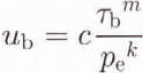
were introduced. Here, ub
is the basal horizontal velocity. ![]() is the basal shear stress, calculated hydrostatically, pe
is the reduced or effective pressure at the base (the excess of ice pressure over buoyant force) and k, m, and c are adjustable parameters. In theoretical treatments, such as Weertman (1964), c may be composed of physical quantities. However, it always contains a roughness parameter that renders it unmeasurable, and hence empirical for the current purpose.
is the basal shear stress, calculated hydrostatically, pe
is the reduced or effective pressure at the base (the excess of ice pressure over buoyant force) and k, m, and c are adjustable parameters. In theoretical treatments, such as Weertman (1964), c may be composed of physical quantities. However, it always contains a roughness parameter that renders it unmeasurable, and hence empirical for the current purpose.
In experiments described here, the values k = 1 and m = n = 3 were set and c was used as a tuning parameter. Calculation of pe required information about the liquid-water content of the glacier. As the hydrology of Storglaciären has been extensively studied, it was possible to estimate the buoyant reduction b in total basal pressure pb as a variable over the glacier, such that
(i.e. basal water pressure is bpb). To specify sliding velocities ub using Equation (5). basal pressures and stresses are calculated hydrostatically, and pe is then calculated from Equation (6) using an assumed horizontal field of b. The buoyancy parameter ranges from b = 0.1 in the accumulation area to b = 0.9 in some of the low er parts of the glacier. As will be seen, the results are not sensitive to this parameter. Once the map of effective pressure-reduction factors was established, it was not modified during the model tuning. Even though it is not well known, it is potentially measurable and therefore not a good tuning coefficient.
The second tuning coefficient for Storglaciären simulations was the viscosity parameter B. In a glacier with significantly varying temperature, Β should be allowed to vary with temperature, as in Reference HansonHanson (1990). On Storglaciären, only the tipper cold layer is below temperate conditions and deformation within this layer is very small. Because of the nearly constant temperature and the lack of other information about variations in Β with crystal fabric or water content, a constant value of Β for the entire glacier has been assumed in all simulations.
Modifying Β and c allowed adjustment of the two major contributors to the surface velocity: the basal sliding and the internal deformation. Since a reasonable match to known velocities was obtained by using a single value of each parameter for the entire glacier, no attempt was made to have these constants vary spatially. These parameters do vary over the glacier, causing some of the inaccuracy of the solution. Additional discrepancies between model and reality arise from imperfect knowledge of the buoyancy and the basal topography. Measured velocities for comparison to the model were taken from two sources. Three-dimensional velocity components were measured at 32 stations during the Storastaknet experiment of 1984–86 (Reference Hooke, Calla, Holmlund, Nilsson and StroevenHooke and others. 1989). These velocities represent annual averages for the glacier. (Numerical values of the Storastaknet velocities were obtained directly from R. L. Hooke. who noted that the vector scale on figure 1a in Reference Hooke, Calla, Holmlund, Nilsson and StroevenHooke and others (1989) is mislabeled. Velocities are twice as high as indicated on that figure and the label “50mm/d” on the scale arrow should be “100mm/d”.) Of the many boreholes drilled during field research on Storglaciären, three, drilled in 1985, 1987 and 1988, respectively, were cased with aluminum tubing for inclinometry experiments (Reference Hooke, Pohjola, Janssen and KohierHooke and others, 1992). Two of these deformation measurements were made only during the Summer in which they were installed. The 1988 hole was also being measured once the following year.
A series of simulations was undertaken for purposes of tuning the values of Β and c. to match best the surface-and borehole-velocity values. The resulting simulation served as a control run for comparison with perturbation experiments. Tuning of Β was confined to increments of 0.02 MPa year 1/n and variation of c was confined roughly to factors of 2. Quantitative comparisons were made between simulated horizontal components of the surface velocity and components from the Storastaknet experiment at roughly the same locations using the vector form of the Reference WillmottWillmott (1982) index of agreement and the vector-regression coefficients from Reference Hanson, Klink, Matsuura, Robeson and WillmottHanson and others (1992). Comparisons of vertical surface velocities and horizontal borehole velocities, and suggestions for direction of tuning, were made using graphs for each run analogous to Figures 2 and 3.

Fig. 2. Scatter plot of agreement between horizontal velocities in the control simulation and Storastaknet observations, including a perfect-correspondence line. Horizontal speeds are indicated with ο, x components with * and y components with +. All speeds are in m year−1.

Fig. 3. Simulated and observed horizontal speeds at locations of three boreholes. Dashed lines are observations and solid lines are the control simulation.
Tuning gave a reasonable lit using B = 0.20 M Pa year 1/n and c = 104 m year−1 MPa−2 (Table 1; Figs 2, 3 and 4). As will be seen in the discussion of sensitivity studies, this control run cannot unequivocally be called a “best” model with respect to all model-validation parameters. It is a good starting point from which to study the effect of perturbations.

Fig. 4. Map of observed Storastaknet surface velocities and corresponding values from the control run. Dots indicate the base of each vector. Solid lines are model simulation and dashed lines are observations.
Table 1. Model evaluation statistics describing the fit between 32 Storastaknet surface velocities and closely corresponding surface nodal points of the control run. All quantities are in m year−1, except than the index of agreement is dimensionless. r.m.s.e. indicates root mean-squared error

The match between the control run and Storastaknet is best in the transverse-velocity components, particularly considering that the largest of these occur where the model has successfully simulated the turning of the flow from the cirque into the central part of the glacier. Modeled velocities consistently over-respond to transverse slopes. This is illustrated by the horizontal convergence in the zone coming out of the accumulation area and the horizontal divergence in most of the rest of the glacier. The transverse errors suggest that simulated compressive longitudinal stresses are too high in most of the glacier.
The fit of the vertical-velocity components is not as good. Vertical-velocity components in two-dimensional versions of this model were the least tunable Reference HansonHanson, 1990), because they are sensitive to small errors in horizontal velocity up-and down-glacier. Furthermore, vertical components of measured velocities have the highest relative error among the components. The pattern of vertical components will receive little further attention except as they relate to vertical stresses.
Longitudinal (or x) components arc the largest and these show a pattern of deviation that could not be removed by any reasonable tuning of Β and c (Fig. 2) Small velocities are underpredicted and large velocities are overpredicted. This is because velocities are generally too large in the steep parts of the lower accumulation zone and too small near the terminus (Fig. 4). Fit of the velocity magnitudes is good through the deepest over-deepened part of the glacier roughly 1400–2500 m in Figure 1b. known as the main overdeepening). A net result of this pattern is that horizontal velocities predicted by the model are somewhat smaller on average than observed ones. Storastaknet locations are biased towards the ablation area, so it is possible that an area-weighted statistic would show better agreement if there were sufficient data in the cirques to justify such an approach.
A further interpretation of the differences in pattern can be made by using vector correlation Table 2) Reference Hanson, Klink, Matsuura, Robeson and WillmottHanson and others. (1992) When used for model comparison, vector correlation produces an overall correlation ρ that is preferred to be close to 1, a dimensionless scale factor β that should also be close to 1, a turning angle θ that is preferably close to zero and an “intercept” term α with the dimensions of the modeled field that should be small. The parameters ρ, β and α are directly analogous to numbers produced by a scalar regression, α is the magnitude of a vector whose direction is of less interest for model intercomparison. The direction of α for the control run to Storastaknet regression is 4.2 ° counter-clockwise from the x direction.
Table 2. Summary of all model runs discussed in the text. The first three numerical columns indicate the applied conditions of stiffness (MPa year1/n), sliding-speed parameter (103m year−1 MPa−2) and water-head fraction. Fit to Storastaknet data is indicated by the vector correlation (ρ), regression-scale factor (β), turning angle (θ, counterclockwise) and magnitude of regression “intercept” (α, m year−1). Velocities averaged over the entire model domain, its surface and its-base are given as average horizontal ![]() and vertical
and vertical ![]() in m year−1
in m year−1

Despite the good overall correlation in this case, the vector-regression parameters significantly vary from their most desirable values. These coefficients can be interpreted as indicating that the measured values will be best approximated by the sum of a constant vector, pointing directly down the main valley at 7 m year−1 (α in Table 2), added to two-thirds of the model-predicted vector magnitude (B), shifted clockwise 14 ° (θ). The vector correlation quantitatively reinforces the interpretation drawn from Figure 2 that the model prediction is too variable. The 14 ° turning angle docs not represent model error but rather can be interpreted as restoring some of the —y-direction component of the prediction that was removed by the small-scale factor.
The velocity-pattern inaccuracy indicates that the model produces too large a longitudinal strain rate. The strain rate can be reduced by increasing the stiffness (B) and hence increasing longitudinal coupling. Increasing Β exacerbates the problem of overall underprediction. Ameliorating that problem with increased sliding decreases the overall fit of the solution, because of increased directional inaccuracy. Additionally, comparison of three available borehole-deformation profiles, while showing significant local errors of magnitude, agree well in deformation with depth (Fig. 3).
Sensitivity Studies
Perturbation runs were generated by simulating the velocity field with tuning coefficients that were slightly different from the control run. These were used to explore the sensitivity of the model results to ice stiffness, basal roughness and internal water pressure. Perturbations of 23 were ±0.02 MPa year 1/n and c was multiplied by 2 and by one-half (all runs summarized in Table 2). Additional sensitivity runs include two that involved combinations of the above perturbations, a series in which b was assumed to be constant over the glacier and one in which sliding was set to zero.
None of the perturbation experiments has a significant effect on the size of the vector correlation, turning angle or intercept magnitude, (manages in sliding have a greater effect than changes in stiffness (reduced sliding improved the fit to observations) but these changes are small enough that the lack of variation is more worthy of note than any changes produced. The pattern of directions shown in the control run (Fig. 5) does not vary to visual inspection in any of the sensitivity runs. Hence, the pattern of the surface velocity is apparently largely fixed by kinematic considerations: the shape of the glacier and the imposition of lateral boundary conditions.

Fig. 5. Control velocity simulation, a. Horizontal surface vectors, b. Horizontal base vectors, c. Vertical vectors. 5 × vertical exaggeration. Every other node in each vertical column was omitted for clarity.
Perturbations had a larger effect on the vector-scaling factor β Changes in stiffness caused the largest responses in the scaling factor and the closely related average velocities. Decreasing stiffness had the obvious effect of increasing the surface velocities. The lack of change in vector correlation, turning angle or intercept magnitude implies that the increase in surface velocity occurred without significant change in the orientation of the surface-velocity vectors.
Responses to sliding changes are consistently smaller than responses to internal stiffness. However, the control run has an average sliding speed of 1.1 m year−1 and an average deformation speed of 7.5 m year−1. Thus, the halving and doubling of sliding speed produced basal perturbations of −0.6 and 1.1 m year−1, respectively, and the resulting surface-velocity changes nearly represent the sum of those basal perturbations with the results of control surface velocity. Similarly, ±10% changes in Β result in 1.1−3 = 0.75 and 0.9−3 = 1.37 changes in viscosity, which approximate the deformation changes produced by the stiffness perturbations.
Changes in stillness have a greater effect on overall velocity than changes in sliding because most of the simulated velocity consists of internal deformation rather than sliding. Surface-velocity changes produced by the model closely follow the simple calculations explained in the previous paragraph. These simple results arc consistent along the entire central flowline (Figs 6 and 7). Surface horizontal velocity profiles from the stiffness experiments (Fig. 6) follow each other for the entire length of the flowline. The pattern is less coherent for the sliding experiments (Fig. 7), as the surface over-responds to the basal forcing through the main overdeepening area (from 1.7 to 2.5 km) but under-responds at the various basal peaks, i.e. changes in the surface-speed curves are substantially greater than changes in the base-Speed curves. These differences in character are reasonable: the stiffness changes are applied uniformly through the ice, so their effects should he more strongly connected to the surface than sliding changes applied only at the base.

Fig. 6. Horizontal speeds along the approximate flowline using three different values of the stiffness parameter B. Lower solid curve is the basal speed applied in all three cases. Upper curves are surface speeds for control run (solid curve. Β = 0.20 MPa year1/n), increased stiffness (short dashes. Β = 0.22 M Pa year1/n), and decreased stiffness (long dashes, Β = 0.18 MPa year1/n).

Fig. 7. Horizontal speeds along the approximate flowline using four different values of the roughness parameter C. Lower curves are sliding speeds and upper curves are surface speeds. The four cases are no sliding (c = 0, dot dashed curve), increased friction (c = 5 × 10³ m year −1 MPa−2, long dashes), control (c =10 × 103 m year−1 MPa−2. solid curve), and decreased friction (c =20 × 103 m year−1 MPa−2, short dashes).
In a third pair of perturbation experiments, contrary effects of sliding and stiffness were combined. No nonlinearities or feed-backs were found and the responses could be explained via a factor applied to the basal velocity plus a factor applied to the deformation, as above. The increased stiffness/decreased friction run is notable as being a good alternative control run. It provides similar overall velocity values as the control, with increased longitudinal coupling and improvements in the values of β and α relative to the control. Nevertheless, it had the worst overall vector correlation with Storastaknet of any of these runs. Comparison of these two runs shows that a model of this complexity cannot be used to refine the viscosity or the sliding law beyond a gross level. Given the contrary responses of the various model-evaluation parameters, one cannot unequivocally argue that the control run is a better simulation of current reality than the increased stiffness/ decreased friction run.
Further perturbation runs examined the value of b. In the control run and the previously discussed perturbation runs, b varied from small values in the firn area to medium values in the ablation area. Rather than shift this pattern up and down by a constant height or a constant factor, perturbation runs were made with constant values of b over the entire glacier. That is a somewhat unrealistic assumption, as it leads to horizontal gradients in the hydraulic potential in the glacier that would not be maintained on average in a real, temperate glacier. However, generalizing knowledge of summer water levels into a pattern that characterizes (he entire year is also somewhat dubious. Choosing a constant b is useful for sensitivity tests in that one can examine both the pattern and the overall magnitude of the internal water-pressure effect.
The constant medium water run closely approximates the control in velocity magnitudes and model-evaluation statistics. This value, b = 0.5, is similar to the values of b used in the variable runs for much of the main overdeepening. Changing from variable b to constant b affects the pattern of velocities only slightly. As with the previous sliding-perturbation runs, the variations in constant b have small, linear effects on the surface velocity (Fig. 8).

Fig. 8. Horizontal speeds along the approximate flowline using four different assumptions about internal water pressure. Lower curves are sliding speeds and upper curves are surface speeds. Cases are control (variable b, solid curve), constant low water (b = 0.3, long dashes), constant medium water (b = 0.5, short dashes), and constant high water (b = 0.7, dot-dashed).
The vector correlation improves slightly as the water-head fraction is lowered, achieving the highest value among all the simulations when sliding is simply set to zero. Storglaciären slides but the direction of its sliding is unknown. In this model, the direction was assumed to be down-gradient of the surface slope. That direction pattern may have degraded the lit to observations of the velocity simulation. Overall, the variations in quality of lit among this set of runs is not large, implying that the exact pattern of internal water pressure docs not have a large effect on the velocity pattern. That would certainly change if water pressure approached overburden pressure, so simulation of the summer velocity Held would require substantially more attention to internal water pressure.
The final variable used for sensitivity studies was the How-law exponent, n. Experiments with n = 2, 2.5, 3.5 and 4 used the control values of B, c and internal water pressure (n = 2 and 4 summarized in Table 2). In this shallow range of glacier thicknesses, increasing n increases the surface speed rather dramatically (Fig. 9). Changing n in this range affected the solution shape roughly m the same manner as changing B, and hence could not be usefully taken as an additional free-tuning parameter.

Fig. 9. Horizontal speeds along the approximate flowline using five different values of the flow-law exponent n. Control-run values of base and surface velocity are shown as solid lines. Dashed lines are surface velocities, labeled With their respective values of n.
Discussion
Simulation Quality
One purpose of this paper is to report the development and testing of the finite-element model. In the period of lime during which this model has been under development, simulations of the sort described here have gone from requiring supercomputers to requiring much less costly “advanced work stations”, resulting directly from improvements in computing hardware. Computing constraints still limited the Storglaciären simulations in resolution and in the number of timing experiments that could be performed. In a sense, this has not been a constraint in this study, as further tuning would have provided little additional insight.
Modeling at this complexity shows how little is really known about a glacier. The simulations made use of a 3 year, all-season velocity survey, three inelinometercd boreholes, surface photogrammetric surveys, radar surveys of basal topography and internal temperature regime, and dozens of boreholes drilled to explore the water system. Similar background could be provided for only a few other Northern Hemisphere “laboratory” glaciers. Yet, the tuning is fairly crude and has provided limits but not specific values for some of the parameters of Storglaciären’s flow.
Model tuning suggests that Β for Storglaciären is 0.20−0.22 MPa year 1/n , consistent with ice a degree or so below freezing in the formula of Reference HookeHooke (1981) and also similar to the value found by Reference Raymond and HarrisonRaymond and Harrison (1988) for Variegated Glacier. This value was found primarily by tuning the finite-element simulation to the shape of the borehole profiles (Fig. 3) and the slope of the one-to-one correspondence line for Storastaknet values (Fig. 2). Since this value range was found by using a constant value over the entire glacier and with no terms deleted from the stress equations solved by the finite-element model, it represents a statistical best estimate of the value of Β under the assumptions of homogeneity, isotropy and n = 3. Given the highly variable longitudinal coupling on Storglaciären indicated in two-dimensional modeling studies (Reference Hanson and HookeHanson and Hooke 1994), the method used here may be the best way to estimate Β for this glacier, even though it is approximate.
The sliding speeds imposed here were substantially smaller fractions of surface velocity than estimated by Reference Hooke, Pohjola, Janssen and KohierHooke and others (1992). The fit of the control run to their borehole data was the primary test used to fix a value for Β based on the deformation of the upper part of the profile (Fig. 3). All three holes show larger observed velocities than modeled velocities and all observations terminate at the bottom with a large speed that was interpreted by Reference Hooke, Pohjola, Janssen and KohierHooke and others (1992) as a sliding velocity. At the locations of the boreholes, the modeled glacier has greater depth than the observed boreholes. The control simulation in each case therefore appears to extend below the observations. This is problematic because the greatest part of the surface velocity in the control simulation arises from deformation within the lowest 30 m or so. Thus, the left 120 140 m of each hole shows good agreement between simulation and observation, despite completely different physical processes near the base.
A variety of possible causes can be invoked for the difference in basal sliding between the data of Reference Hooke, Pohjola, Janssen and KohierHooke and others (1992) and the current simulations. Hooke and others discussed the possible sources of error in their data collection and reduction procedures, and those errors are not large enough to appreciably diminish the current discrepancy. A substantial improvement in agreement would be obtained if they seriously underestimated the size of their basal layer, which is also unlikely. The importance of that possibility is shown by the difference in sliding-speed percentages between hole 85–2, which had a 17 m basal layer (∼90% sliding), and the other holes that were inferred to be at the bottom of the ice (∼60 75% sliding). Most of the borehole-deformation data were collected within the summer season, whereas the simulations here are for the slower speeds expected of an annual average. Nevertheless, deformation measurements in hole 88–4 spanned a full year and agreement is not appreciably better there. If the modeled velocities at these points were increased by adding sliding in amounts of the seasonal accelerations in the Storastaknet experiment, the sliding percentages would still be well below half those expected.
One conclusion of Reference Hooke, Pohjola, Janssen and KohierHooke and others (1992) was that the onset of sliding in the summer, while important, did not have an overwhelming effect on the deformation profiles, indicating that tuning to the shape of the upper parts of the deformation profiles was not an incorrect procedure. One clear discrepancy is that the nodal columns of the model grid that were used for comparison to the boreholes all had thicker ice than was inferred from the field data. Basal heights used in the model were taken from the radio-echo soundings map of Reference ErikssonEriksson (1990), which did not consistently use borehole-drilling depths for leftographic control. Substantially larger sliding speeds as a percentage of surface speed would have required increasing B, producing poorer fits to the longitudinal strain field and the deformation of the upper parts of the cased boreholes. Thus, a truly satisfying explanation for the discrepancy between the sliding values of Reference Hooke, Pohjola, Janssen and KohierHooke and others (1992) and this simulation remains elusive at this point.
Stress Fields
An interesting feature of Storglaciären’s dynamics is the combination of lateral freezing and bottom sliding, a combination that seems to have eluded previous analytical treatment on simplified geometries. An advantage of the finite-element model is that all six terms of the stress tensor can be calculated from the model solution. We can therefore see how stresses in the model vary from the simplest theoretical stress fields. (Stresses calculated as averages over an element, using the same partial derivative and integration procedures as in the model, will exactly reproduce the stress field implied by the model solution even though those stresses never explicitly appear in the model calculations.)
Stress-tensor components calculated from model output provide a means of calculating force-balance components discussed by Reference Van der Veen and WhillansVan der Veen and Whillans (1989). Using the model geometry and stress tensors in the basal elements, one may calculate driving stresses and basal resistances, ![]() and
and ![]() , from
, from

and

in which zs and zb are surface and basal height, respectively. When these stress components are plotted as if vectors in the horizontal plane, their differences denote the magnitude of non-local forcing at each point (Fig. 10). (In Figure 10, especially note that directions of basal resistances have been reversed so that these vectors are more directly comparable to the driving stresses. A vector drawn from the tip of the basal-resistance (dotted) vector to the tip of the driving-stress vector would represent the stress due to non-local forces at each point.) These vectors indicate that through the main overdeepening, resistance via side drag is nearly hall that of basal drag and these drags add up to considerably more than the driving stress at this point. Driving stresses above the main overdeepening (in the convergence zone of the two cirques) substantially exceed basal resistance. The balancing of these stresses is most easily explained by compression against the main overdeepening and riegel below but one should also note the substantial contribution of side drag apparent in the main overdeepening. where driving stresses have essentially no down-glacier component but are nevertheless accompanied by a substantial basal resistance.

Fig. 10. Vectors of driving stress (![]() , solid lines) and basal resistance (
, solid lines) and basal resistance (![]() , dotted lines). Dots represent center points of basal elements and are the bases of the vectors. Basal resistances have reversed direction for easier comparison to the driving forces (see discussion in text).
, dotted lines). Dots represent center points of basal elements and are the bases of the vectors. Basal resistances have reversed direction for easier comparison to the driving forces (see discussion in text).
The buttressing of the glacier by its sides and other effects of its geometry are visible on maps of the vertically integrated deviatoric stress components (Fig. 11). Each of the maps in Figure 11 shows ![]() for the indicated component. Values are shown as the model “sees” them, as constants across each element column
for the indicated component. Values are shown as the model “sees” them, as constants across each element column
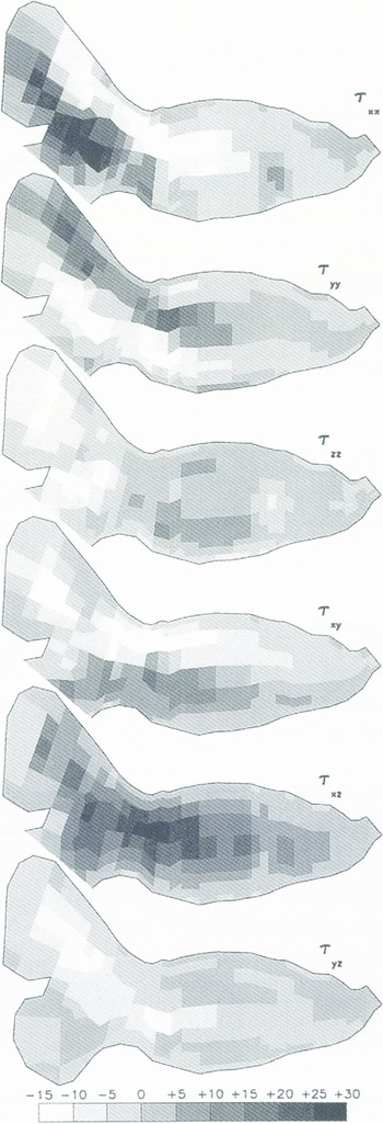
Fig. 11. Vertically integrated stress components in each element column. All values in the smith cirque were small, so they have been mostly eliminated to aid in graphical clarity. Dimensions are M Pam, or M Nm−1.
As might be expected, the highest stresses over the largest area are found in vertical shear in the direction of motion, shown by high positive values of ![]() through most of the glacier and high negative values of
through most of the glacier and high negative values of ![]() in the north cirque. These forces are slope-driven, with highest values occurring in steeply sloped areas coming out of the high part of the north cirque and in the transition zone between the firn area and the ablation area. They directly affect the patterns of extension and compression shown in
in the north cirque. These forces are slope-driven, with highest values occurring in steeply sloped areas coming out of the high part of the north cirque and in the transition zone between the firn area and the ablation area. They directly affect the patterns of extension and compression shown in ![]() and
and ![]() . Particularly,
. Particularly, ![]() shows extension behind and compression ahead of the area of high negative
shows extension behind and compression ahead of the area of high negative ![]() in the north cirque, and
in the north cirque, and ![]() shows a more intense pattern of extension behind and compression ahead of the area of high
shows a more intense pattern of extension behind and compression ahead of the area of high ![]() in the transition zone. The latter compression extends through the main overdeepening and ends at the riegel, implying that the entire main overdeepening receives a substantial shove from the slopes coming out of the firn area.
in the transition zone. The latter compression extends through the main overdeepening and ends at the riegel, implying that the entire main overdeepening receives a substantial shove from the slopes coming out of the firn area.
Positive ![]() to the right of center and negative
to the right of center and negative ![]() to the left of center represent the normal pattern for any glacier but these lateral shear stresses are large in this case. Lateral shear in the upper part of the ablation zone is comparable to the vertical shear through most of the lower part of the ablation zone. These shear stresses are substantially larger than the longitudinal compression. The center line of the side-drag field is to right of center through most of the ablation zone. This asymmetry is caused by the left turn made by the main flow of the glacier between the north cirque and the ablation zone. The glacier exhibits an “overshoot” in which ice builds up on the right side of the glacier to accomplish the turning, enhancing the lateral drag on the right side. The force required to turn the main flow also shows up in the pattern of extension and compression in
to the left of center represent the normal pattern for any glacier but these lateral shear stresses are large in this case. Lateral shear in the upper part of the ablation zone is comparable to the vertical shear through most of the lower part of the ablation zone. These shear stresses are substantially larger than the longitudinal compression. The center line of the side-drag field is to right of center through most of the ablation zone. This asymmetry is caused by the left turn made by the main flow of the glacier between the north cirque and the ablation zone. The glacier exhibits an “overshoot” in which ice builds up on the right side of the glacier to accomplish the turning, enhancing the lateral drag on the right side. The force required to turn the main flow also shows up in the pattern of extension and compression in ![]() , the negative values of
, the negative values of ![]() on the right and the vertical extension shown in
on the right and the vertical extension shown in ![]() just below the firn area at the bead of the main overdeepening.
just below the firn area at the bead of the main overdeepening.
Conclusions
Simulations of Storglaciären’s velocity field with a three-dimensional finite-element model required values of the stiffness parameter Β of 0.20−0.22 M Pa year 1/n to match observed characteristics of horizontal and vertical strain rates. Sliding speeds necessary to match surface velocities were set much lower than would have been expected from borehole studies. Analysis of the stress field showed that the main driving forces for the glacier come from areas of steep slope in the firn area and at the head of the ablation area. Because the glacier is frozen to its sides, lateral drag accounts for a greater amount of the total resistive force than might be expected for a temperate glacier.
The weakest feature of these simulations is probably the uncertainty over basal sliding. Simulations were insensitive to the exact form of the basal sliding law and basal roughness parameters, in part because sliding was such a small proportion of the total speed of the glacier and parameters controlling sliding were not allowed to vary spatially as much as is probably the case in nature. For further analysis, it seems necessary to produce sliding in the model as a natural result of the applied basal stress and the coupling of the ice to the bed at each point. That will require further model development.
Acknowledgements
Tins paper could not have been completed without many discussions about the dynamics of Storglaciären with R. Hooke. who also provided numerical values lor Storastaknet and borehole data that have only been published in graphical form. Computing was assisted by U.S. National Science Foundation grant OPP-9224175 and by substantial allocations from the University of Delaware’s Computing and Network Services.


