


Introduction
Glacier surges are cyclic phenomena whereby glaciers switch between periodic phases of low activity with slow ice flow during a century- to decadal-long ‘quiescent’ phase, and rapid flow during a short-lived peak (‘surge’ phase) where velocities increase by a factor of 10–1000 times (Meier and Post, Reference Meier and Post1969; Murray and others, Reference Murray, Luckman, Strozzi and Nuttall2003a). While only ~1% of the glaciers in the world are thought to be of surge-type (Jiskoot and others, Reference Jiskoot, Boyle and Murray1998; Sevestre and Benn, Reference Sevestre and Benn2015), the Svalbard archipelago contains one of the densest population of such glaciers in the world with estimates varying between 13% (Jiskoot and others, Reference Jiskoot, Boyle and Murray1998) and 54–90% (Lefauconnier and Hagen, Reference Lefauconnier and Hagen1991). Small glaciers and ice caps are expected to be large contributors to sea-level rise in the near-future (Zemp and others, Reference Zemp2019), and from Svalbard, tidewater glaciers are the largest contributors (Nuth and others, Reference Nuth, Moholdt, Kohler, Hagen and Kääb2010). Hence, a better understanding of surge-type tidewater glaciers in Svalbard that have the ability to quickly discharge large ice masses into the ocean will provide more accurate sea-level projection from this region.
Similar to most Arctic tidewater glaciers, Svalbard glaciers also lose most of their mass through frontal ablation (calving + submarine melt) (e.g. Rignot and others, Reference Rignot2008; Błaszczyk and others, Reference Błaszczyk, Jania and Hagen2009; Burgess and others, Reference Burgess, Forster and Larsen2013; Van Wychen and others, Reference Van Wychen2014; Khan and others, Reference Khan2015; McNabb and others, Reference McNabb, Hock and Huss2015). In Svalbard, historical synthesis of remote-sensing studies has shown that marine-terminating surge-type glaciers commonly have different surge behaviour than land-terminating surge-type glaciers (Murray and others, Reference Murray, Strozzi, Luckman, Jiskoot and Christakos2003b), although this does not exclude that both types can be explained by the same theoretical principles (Sevestre and Benn, Reference Sevestre and Benn2015). Earlier studies on tidewater glaciers in Svalbard and in particular on Osbornebreen, Fridtjovbreen and Monacobreen (Hodgkins and Dowdeswell, Reference Hodgkins and Dowdeswell1994; Rolstad and others, Reference Rolstad, Amlien, Hagen and Lundén1997; Luckman and others, Reference Luckman, Murray and Strozzi2002; Murray and others, Reference Murray, Strozzi, Luckman, Jiskoot and Christakos2003b) have suggested that the surge initiates over the lower part of the glacier and then spreads over the entire glacier surface based upon the evolution of surface velocities and crevasses patterns. Down-glacier surge initiation and up-glacier spread of surface velocities was also observed on Sortebrae, a tidewater glacier in East Greenland, albeit with various propagation nuclei (Pritchard and others, Reference Pritchard, Murray, Luckman, Strozzi and Barr2005). By contrast, on land-terminating glaciers in Svalbard such as Usherbreen and Bakaninbreen (Hagen, Reference Hagen1987; Murray and others, Reference Murray, Dowdeswell, Drewry and Frearson1998), the active surge starts from the upper accumulation area following a surge front travelling down glacier, which is similar to observations from Variegated Glacier and Trapridge Glacier in Alaska and Yukon (Clarke and others, Reference Clarke, Collins and Thompson1984; Kamb and others, Reference Kamb1985; Frappé and Clarke, Reference Frappé and Clarke2007).
Despite the potentially large number of surge-type tidewater glaciers in Svalbard (Błaszczyk and others, Reference Błaszczyk, Jania and Hagen2009), the typically long periods between the active phases have historically given few opportunities to study repeating surge events in detail (Mansell and others, Reference Mansell, Luckman and Murray2012). However, more recent surge events and the improved availability of remotely sensed data have yielded higher spatial and temporal observations in the time leading up to an active surge on such glaciers. Evidence from these events shows that the active surge phase initiates after a frontal destabilization (Strozzi and others, Reference Strozzi, Kääb and Schellenberger2017; Sevestre and others, Reference Sevestre2018; Willis and others, Reference Willis2018; Nuth and others, Reference Nuth2019). During the destabilization, crevassing often initiates or intensifies close to the terminus and propagates up-glacier (Flink and others, Reference Flink2015; Sevestre and others, Reference Sevestre2018). Crevasses have been shown to be able to cause a cycle of positive feedbacks in glacier dynamics by increasing surface melt-water input to the glacier bed, a feedback that was documented in detail during the surge on Basin-3 of Austfonna (Dunse and others, Reference Dunse2015), and has been observed on other glaciers (e.g. Gilbert and others, Reference Gilbert2020). Because the accelerating destabilization prior to the active surge probably only lasts for a few seasons on Svalbard tidewater glaciers, high temporal resolution analysis is necessary to understand both how the destabilization begins and further evolves.
In 2016, an active surge occurred on Negribreen, a tidewater glacier located on the eastern coast of Svalbard (Fig. 1). The surge activated after a frontal collapse, with a signature similar to the collapse of the Nathorst Glacier System (NGS) (Nuth and others, Reference Nuth2019) or Stonebreen (Strozzi and others, Reference Strozzi, Kääb and Schellenberger2017). With remotely sensed data, this paper documents the Negribreen surge event by investigating the dynamic evolution of the glacier via surface velocities, elevation changes, surface structural changes and external conditions, including sea-ice and ocean surface temperatures. We map out a timeline of the dynamic evolution by dividing the surge cycle into four stages, from which we discuss how Negribreen evolved towards an active surge.
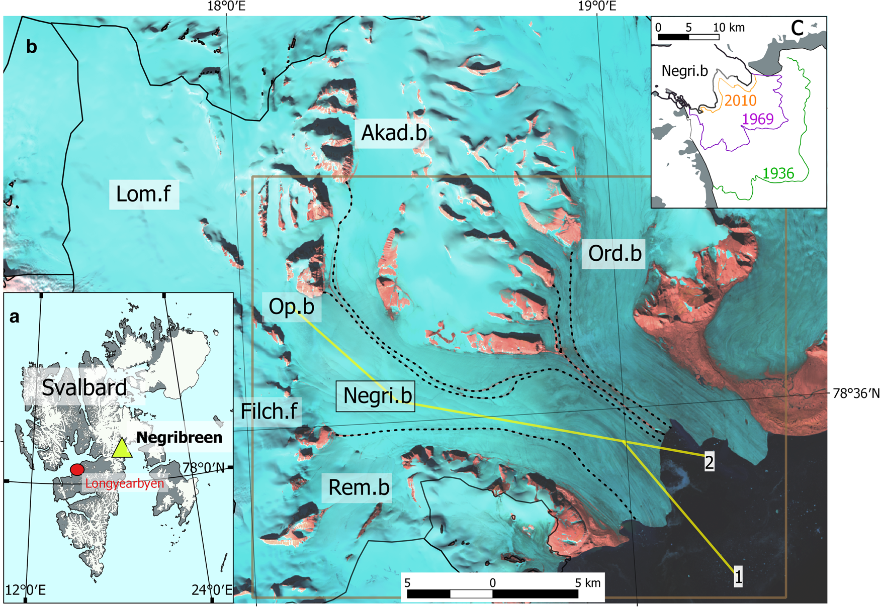
Fig. 1. (a) Map of Svalbard. (b) Overview of the Negribreen Glacier System: location of Negribreen (Negri.b) and neighbouring glaciers Ordonnansbreen (Ord.b), Akademikarbreen (Akad.b) and Rembebreen (Rem.b) are indicated as well as reservoir area Filchnerfonna (Filch.f) and main reservoir Lomonosovfonna (Lom.f), connected to Negribreen through Opalbreen (Op.b). Background image is a summer 2015 Landsat-8 scene and black dashed lines designate glacier boundaries. The brown box represents the approximate extent of maps in other figures. The yellow lines show location of the two centreline profiles used to extract velocity and elevation (line no. 1 for Stage 1 and no. 2 for Stage 2–4). (c) Outline of the glacier in 2015 in black with general retreat patterns since the last surge in 1936 in colour.
Study area
According to radio echosounding investigations from Dowdeswell and others (Reference Dowdeswell, Drewry, Liestøl and Orheim1984), Negribreen is polythermal with a layered cold to temperate thermal ice column. The glacier has two reservoir areas: Filchnerfonna and a section of Lomonosovfonna (main reservoir), which are both connected to the glacier through Filchnerfallet and Opalbreen, respectively (Fig. 1). The Negribreen terminus drains into Storfjorden in Olav V and Sabine Land along with the neighbouring glaciers Ordonnansbreen, Akademikarbreen and Rembebreen. These glaciers, along with some smaller unnamed tributaries, make up the Negribreen Glacier System. In total, this covers an area of 1180 km2, making it one of the largest glacier systems on the island of Spitsbergen.
The last time Negribreen surged is thought to be between 1935 and 1936 (Liestøl, Reference Liestøl1969; Lefauconnier and Hagen, Reference Lefauconnier and Hagen1991). Photos and observations from that time show a significant advance and visible crevasses in the accumulation areas of Negribreen, Akademikarbreen and Ordonnansbreen, suggesting that most of the glacier systems contributed to the terminus advance at that time (Lefauconnier and Hagen, Reference Lefauconnier and Hagen1991). Liestøl (Reference Liestøl1969) estimated that the front advanced with an average speed of 35 m d−1. Recent sea-floor mapping shows mostly fine-grained sediments beyond this surge and suggests that the 1936 terminal moraine position is most likely the largest extent of Negribreen during the Holocene (Ottesen and others, Reference Ottesen, Dowdeswell, Bellec and Bjarnadóttir2017). After the last surge, aerial images show little signs of surface deformation and the terminus has been in continuous retreat (Lefauconnier and Hagen, Reference Lefauconnier and Hagen1991). Outside of Negribreen's 2010 extent, eskers are present on the sea-floor which prolong out in the fjord up to the 1969 extent, indicating that there has been an efficient subglacial drainage system for at least the last decades (Ottesen and others, Reference Ottesen, Dowdeswell, Bellec and Bjarnadóttir2017) while the front position has been retreating (Nuth and others, Reference Nuth2013).
Data and methods
Glacier surface velocities
To get a sufficient temporal coverage of surface velocities, we used data from several sources (Table 1). The earliest observations come from the European Remote Sensing (ERS) satellites ERS-1 and ERS-2 using their tandem-mode observations in 1995 and 1997, which we have processed using standard single-azimuth differential interferometry using the GAMMA radar software (i.e. co-registration, formation of interferogram, flattening, removal of topographic phase, unwrapping; e.g. Luckman and others, Reference Luckman, Murray and Strozzi2002). In contrast to tracking, simple radar interferometry provides only one velocity component in the satellite looking direction (line of sight). We also used standard offset tracking on a RADARSAT-1 radar image pair of 11 March–4 April 2008 (e.g. Schellenberger and others, Reference Schellenberger, Dunse, Kääb, Kohler and Reijmer2015).
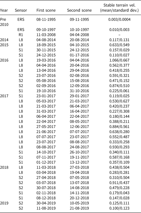
Table 1. Overview of the data acquisitions used for surface velocity extraction and their stable terrain velocities. Data from several sensors were needed to get sufficient information to produce a timeline of events. Data sources include the European Remote Sensing satellites (ERS), RADARSAT-1 (R1), Landsat-8 (L8), Sentinel-1 (S1) and Sentinel-2 (S2)
A timeline with higher temporal resolution was created for 2014–18. Within the day-lit months (approximately March through October), surface velocity data mostly come from the Global Land and ice Velocity Extraction (GoLIVE) dataset (Fahnestock and others, Reference Fahnestock2016; Scambos and others, Reference Scambos, Fahnestock, Moon, Gardner and Klinger2016). The GoLIVE velocity fields are created by normalized cross-correlation (NCC) on a sampling grid of 300 m, based on the Landsat-8 panchromatic bands. All fields covering Negribreen with a path between 209 and 219 and row 003 or 004 (WRS-2 path/row grid system) were downloaded and re-projected to WGS84/UTM33N. We used the highest temporal resolution available with a 16 d repeat cycle and the recommended correlation threshold of 0.3 (Sam and others, Reference Sam, Bhardwaj, Kumar, Buchroithner and Martín-Torres2018). To supplement this dense velocity record and fill potential gaps during polar day, we used additional Sentinel-2 optical data to achieve even higher temporal resolution. For specific implementation details, see (Altena and others, Reference Altena, Haga, Nuth and Kääb2019).
To obtain surface velocities during polar night or whenever light conditions were insufficient, we used Sentinel-1 C-band synthetic aperture radar (SAR) data. A total of 15 image pairs were downloaded from Sentinel Open Access Hub and velocity fields were generated using the Sentinel Application Platform (ESA, 2019). Before offset tracking, we applied orbital files and co-registered image pairs with the Altimeter Corrected Elevations Global Digital Elevation Model (ACE GDEM; Berry and others, Reference Berry, Pinnock, Hilton and Johnson2000). The GRD-format amplitude images were also calibrated so that the pixel values represent radar backscatter values. Velocities were estimated using NCC image matching on subset views covering only Negribreen. The window dimension used was 300 m in both azimuth and range spacing. This makes the search box large enough so that texture, not noise, is matched, but also not too large, which would degrade the matching accuracy under the presence of spatial velocity gradients.
To estimate the uncertainty in the velocity measurements, we selected multiple regions over assumed stable terrain and averaged the displacement values for each image pair. We found that all Sentinel-1 image pairs had stable ground velocities below 0.5 m d−1. In general, the stable terrain velocities from Sentinel-2 and Landsat-8 also gave values below 0.5 m d−1, but were in some cases higher in the range of 0.5–1 m d−1. During some periods, we found these sources of error to be significant. For instance, for the pre-surge image pair covering 18 September–4 October 2015, the average displacement over stable ground exceeded some of the measured on-glacier velocities. However, the fact that we have multiple measurements showing the same underlying trend lends confidence to the velocity measurements.
Digital elevation models
To study elevation and elevation changes on Negribreen, we use digital elevation models (DEMs) derived from multiple sources (Table 2). The earliest DEM we have available is photogrammetrically derived from aerial photos acquired in 1969 over the lowermost zone of the glacier, processed by the Norwegian Polar Institute (NPI). Additionally, we used a DEM produced by NPI from aerial photos acquired in 1990, which covered most of the Negribreen system.
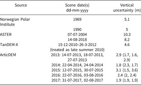
Table 2. DEMs used for elevation changes. To increase the spatial coverage of the ArcticDEM strips, we mosaicked strips acquired within a short time of each other; uncertainties reported for both the mosaicked product, as well as the individual strips in parentheses
Most of the later DEMs we have used are from optical stereo satellite imagery such as the Advanced Spaceborne Thermal Emission and Reflection Radiometer (ASTER) (e.g. Toutin, Reference Toutin2008) and ArcticDEM strips (Porter and others, Reference Porter2018). ASTER DEMs are processed using MicMac ASTER (MMASTER Girod and others, Reference Girod, Nuth, Kääb, McNabb and Galland2017) with jitter correction performed by comparisons to the ArcticDEM v3.0 mosaic.
Finally, we used the TanDEM-X Intermediate DEM (IDEM; Balzter and others, Reference Balzter, Baade and Rogers2016) product over Negribreen, resampled from 12 to 30 m resolution. This DEM is a mosaicked product of six separate acquisitions between 15 December 2010 and 26 March 2012. Five of these acquisitions are from December 2010 and January 2011, with the final acquisition from March 2012. The X-band radar signal penetrates dry snow to an unknown depth of up to a few metres, resulting in a negative bias as the elevation values represent a surface that is below the actual snow surface (e.g. Dehecq and others, Reference Dehecq2016). Because most of the acquisitions come from winter 2010/2011, we assume that the elevation reflects the surface conditions of late summer 2010.
To achieve minimum biases in the elevation differences, we co-registered all DEMs using the same methodology as Nuth and Kääb (Reference Nuth and Kääb2011). Before applying this method, we re-sampled all data to 40 m resolution and re-projected them to the same coordinate system (WGS84/UTM33N). The co-registration process was done using the ArcticDEM mosaic as a reference, as it has consistent high-quality coverage over the study area. Due to the narrow spatial coverage of the ArcticDEM strip files, we created mosaics of 2–3 co-registered strips that were acquired relatively close in time (Table 2) using bilinear resampling.
The final root mean square error (RMSE) comparison over stable terrain shows that the ArcticDEM strip files have the highest accuracy, with errors ~2.5 m. Uncertainties for the NPI DEMs and the IDEM are ~5 m while the ASTER scenes have the lowest accuracy, with RMSE values of 10.3 and 8.2 m for the 7 July 2004 and 14 August 2018 acquisitions, respectively.
We used the following equation to estimate the uncertainty in elevation change calculated by differencing two individual DEM products:

where ɛ a and ɛ b are the vertical uncertainties in the older and newer DEM, respectively, and t is the time difference in years between the product acquisition dates.
We find that the error propagation of the vertical uncertainties is in fact significant for DEM differences when the rate of elevation change is small and the time interval between products is short. For example, during the 1990–04 and 2004–10 periods, vertical uncertainties of 1.09 and 2.48 m a−1, respectively, exceed the measured elevation change rates over the entire glacier. Even for the ArcticDEM strip files, which have higher accuracy, uncertainties are still significant in the upper portions of the glacier between 2010 and 2016, as elevation change rates are still low. After 2016, the elevation change is significant, exceeding the vertical uncertainties. We do acknowledge the limitation of these uncertainties. However, similar to the velocity-related errors, we have more confidence in the data through the confirmation of several calculations which show a underlying trend, at least in a qualitative way. We argue that these differences are sufficient for this study.
Driving stress
As there are only sparse measurements of bed topography and ice thickness available for Negribreen, we used a simple calculation to get an indication of driving stress τb:

where ρ is ice density (assumed to be 917 kg m−3), g is the gravitational acceleration (9.8 m s−2), h is the ice thickness and α is the surface slope.
To estimate ice thickness, we subtracted the radio echo sounding profile of bed elevation collected in 1980 by Dowdeswell and others (Reference Dowdeswell, Drewry, Liestøl and Orheim1984) from DEM surface elevations. We restricted this calculation to follow this profile, which is approximately along the glacier centreline. We calculated average driving stresses for two intervals of 2 km length each along this profile, one at the front portion of the glacier and another further up-glacier. We averaged estimated ice thickness from three sample points along each interval and averaged surface elevation and slope from DEMs to approximate driving stress.
Glacier length changes and crevasses
We manually digitized ice front positions from aerial photographs and satellite imagery acquired between 1969 and 2017. Additionally, we digitized approximate front positions pre-1969 based on mapped positions presented by Lefauconnier and Hagen (Reference Lefauconnier and Hagen1991). To estimate length changes, we used the so-called ‘box method’ (e.g. Moon and Joughin, Reference Moon and Joughin2008; Howat and others, Reference Howat, Box, Ahn, Herrington and McFadden2010), as this method yields a less arbitrary measure of length than estimates along a single centreline location.
We also manually outlined crevasse expanse using Landsat and ASTER imagery from 2004 to 2019. Further information about crevasses in the 1990s was obtained by visually interpreting radar backscatter in ERS images.
Sea surface conditions
Fjord or ocean conditions can have a significant impact on calving behaviour, either through amplifying calving from increased ocean temperature (Luckman and others, Reference Luckman2015) or by ice mélange buttressing the glacier (Todd and Christoffersen, Reference Todd and Christoffersen2014). In our investigation, we examined two ocean surface variables such as sea-ice concentration and sea surface temperature close to the terminus of Negribreen. We used monthly averaged reanalysis products between 1990 and 2018 provided by the Arctic Marine Forecasting Center, available at http://marine.copernicus.eu/.
The sea surface temperature assimilated dataset combines observations from infrared sensors, microwave sensors and in situ data from ships and surface drifting buoys, provided by the European Space Agency Sea Surface Temperature Climate Change Initiative (ESA SST CCI). It has a spatial resolution of ~6 km. The sea-ice fraction dataset is obtained from Special Sensor Microwave/Imager (SSM/I) at The Ocean and Sea Ice Satellite Application facility (OSI SAF). This has a sampling grid of 12.5 km, which is used to be consistent with other operational OSI SAF products. However, this sampling grid does not represent the true spatial resolution of the product. The dataset already had a correction for coastal effects, since the radiometric signature of land is similar to sea ice at the wavelengths used for estimating sea-ice concentration. The pixels used to extract data from both products were more than 10 km from land, and we expect only a coarse interpretation of sea surface conditions outside Negribreen. More information about these datasets can be found in Sakov and others (Reference Sakov, Counillon, Bertino, Finck and Renkl2015).
Observations and interpretation
In this section, we present the dynamic evolution of Negribreen since 1969. Through interpretation, mainly of surface velocities and elevation changes, we have divided our observations into four stages based on changes in glacier behaviour. A total overview of the stages can be seen in Figure 2. The stages are in relation to the frontal collapse that occurred on Negribreen in early 2016, which is where we interpret the active surge phase to start.
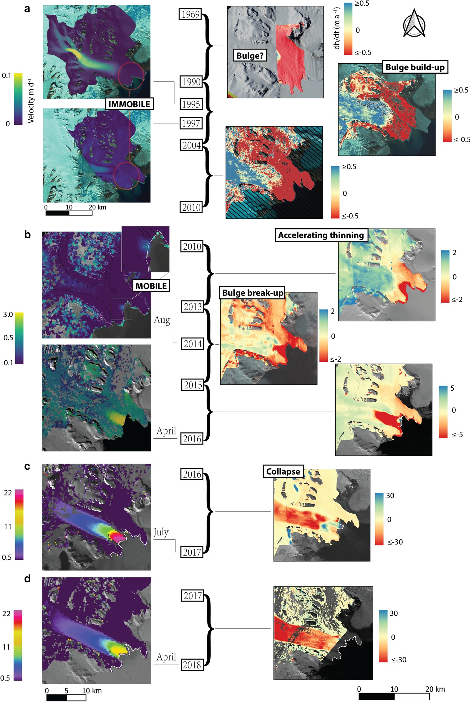
Fig. 2. A timeline of the surge on Negribreen, divided into stages of dynamic behaviour. Left column shows surface velocities given in metres per day (not corrected for stable ground velocities), and right column shows elevation differences given in metres per year. (a) Stage 1, bulge build-up and frontal thinning. (b) Stage 2, dynamic initiation towards the glacier front. (c) Stage 3, collapse and onset of active surge. (d) Stage 4, velocity deceleration.
Stage 1, Pre-collapse: long-term surface geometry change
Elevation change mapping shows that Negribreen underwent a persistent long-term change in surface geometry, which includes thinning towards the terminus and a gradual thickening further up-glacier (Figs 2a and 3b). Between 1969 and 1990, thinning affected the lower portion of the glacier and continued throughout 1990–04 and 2004–10. The thinning rates measured in all sub-periods have approximately similar values. Between 1969 and 1990, the thinning rates were ~3 ± 0.5 m a−1 closest to the terminus, gradually decreasing to 0 m a−1 ~9 km from the terminus. Between 1990 and 2004, the surface at the front thinned at 1 ± 1 m a−1, approaching zero 8 km from the terminus, and in 2004–10 areas close to the terminus thinned by ~3 ± 2.5 m a−1, reaching equilibrium ~9 km from the terminus.

Fig. 3. Centreline data on Negribreen during Stage 1. Shaded colour are respective data uncertainties. (a) Velocities in metres per day from ERS interferometry during a 1 d interval in 1995 and 1997. Note that the ERS velocities have different look-directions. (b) Elevation changes in metres per year between elevation products, 1969–2010. The black horizontal bars show no change. (c) Surface slope and averaged local driving stress values in 1990 and 2010.
Up-glacier from the thinning area, the surface showed a gradual increase in elevation since at least the 1990–04 and 2004–10 periods, with ranges between 0 − 0.5 and 0 − 1 ± 2.5 m a−1, respectively. The limited DEM coverage from the 1969 dataset makes it difficult to investigate this area pre-1990, but we still see elevation changes approaching 0 m a−1 in the same location as in the 1990–04 and 2004–10 differences. This could indicate that surface elevation was increasing pre-1990, although the limited DEM coverage makes any conclusions difficult.
Over time, the elevation changes resulted in a modification of the glacier's geometry, with long-term thinning and steepening of the front since at least 1969, and a small bulge development. From Figure 2a, the extent of the bulge seems to have little spatial fluctuation, and the steepening is most profound in the areas closest to the bulge front, ~7–9 km from the terminus (Fig. 3c). The surface slope in this area increases from values ranging between 1.5 and 2.5° in 1990 and up to 3.5° in 2010. The average driving stress at this area shows a 1.25-fold increase from 58 kPa in 1990 to 73 kPa in 2010 (Fig. 3c). At 13–15 km from the terminus, ~3–5 km up-glacier from the bulge front, we see little change in slope and driving stresses are more or less constant with 46 kPa in 1990 and 43 kPa in 2010.
Interferometric surface velocity from the ERS satellites in 1995 and 1997 provides further important observations of Stage 1 (Figs 2a and 3a). In both acquisitions, velocities are especially low, likely because the acquisitions are from early winter. These velocities are in the satellite's look direction, which conveniently is along the flow direction in the accumulation area for the 1995 pair, and along flow in the ablation area for the 1997 pair. Both of these velocity snapshots together show the existence of mobile ice in the accumulation area, and mostly immobile ice towards the glacier front. Additional velocity measurements from offset tracking in 2008 RADARSAT data show no real difference to the 1995/1997 measurements, with very low velocities (< 0.05 m d−1) at the glacier front, increasing to ~0.12 m d−1 in the ablation area. All of this suggests the presence of high basal friction near the glacier front, a likely factor in the bulge development as the zone of higher friction may have been acting as a barrier for the mobile ice coming from the accumulation area, thus forcing the surface to ‘pile up’.
In the 1995 velocity field, which has a greater coverage of the glacier, highest velocities are seen on Opalbreen, ~25 km from the terminus of Negribreen. This narrow valley glacier acts as a funnel between Negribreen and Lomonosovfonna, the main reservoir area. Here, we also see a consistent presence of crevasses throughout Stage 1 (e.g. ASTER scene from 2004, Fig. 4a), another indication of mobile ice. The mobile nature of the upper basin of Lomonosovfonna suggests that this area has been acting as a source of ice contributing to the bulge development. In the southern part of this reservoir where elevation data are available between 1990 and 2014, we detect a distinct area of surface thinning (Fig. 5b). It covers a surface of 27 km2 with a mean thinning rate of 1.4 m a−1 and a cumulative elevation loss of 33.6 m. This area could be representative of such a source of ice, and similar thinning might have occurred elsewhere on the upper basin of Lomonosovfonna. However, this specific area touches the drainage divide of the upper basin of Tunabreen, another known surge-type tidewater glacier (Flink and others, Reference Flink2015). Therefore, it is unclear if the outflow from this specific area contributed completely to the bulge of Negribreen, flowing east, or partly to Tunabreen, flowing south.
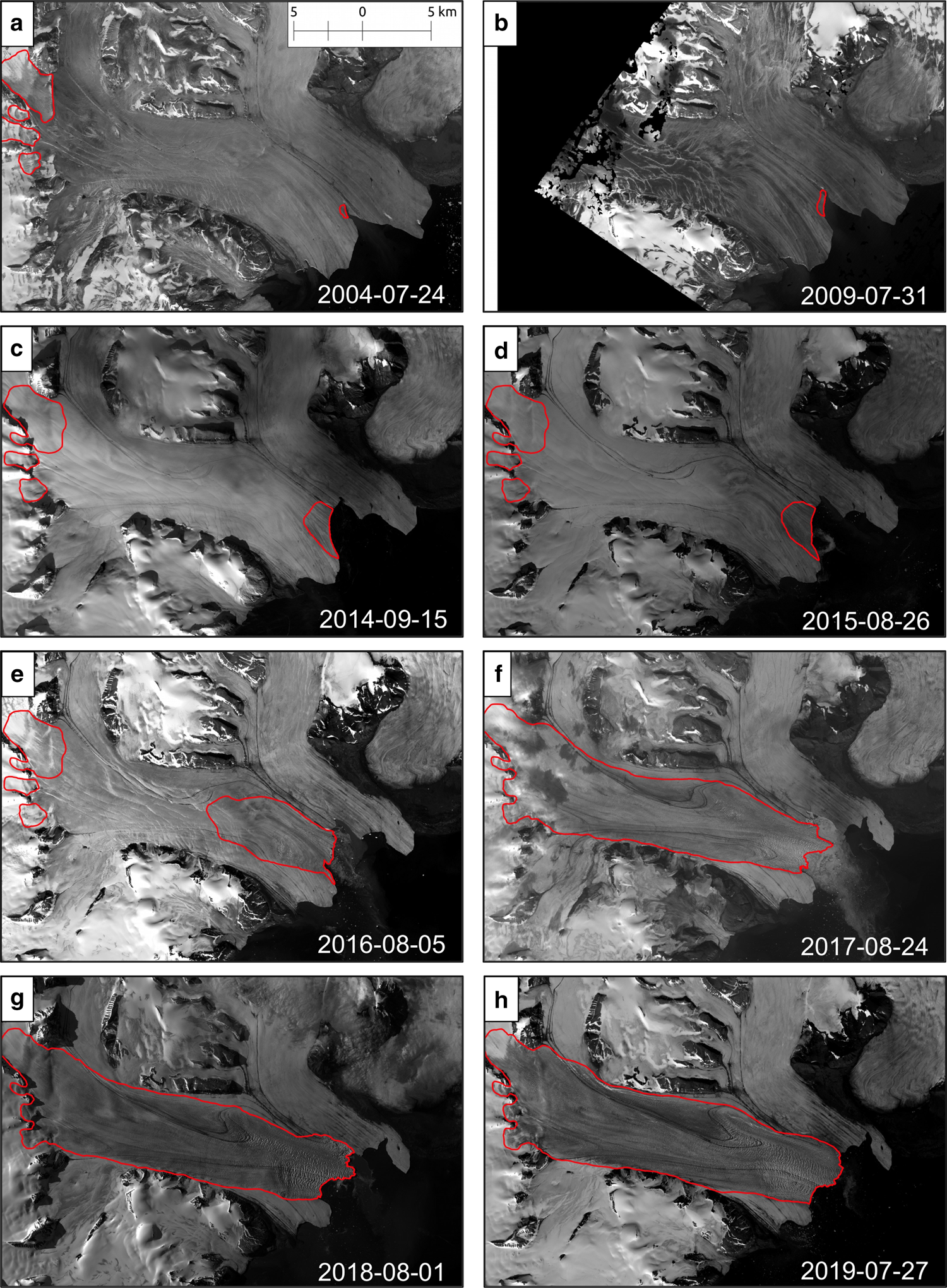
Fig. 4. Extent of visibly crevassed areas (red outline) as digitized from ASTER (a, b) and Landsat 8 (d–h) imagery acquired on the dates shown.

Fig. 5. (a) Surface velocities from ERS interferomtery in metres per day from 1995. (b) Elevation differencing between 1990 and 2014 in m a−1. Together the figures highlight an area of mobile ice on the Lomonosovfonna reservoir area.
Between 1969 and 2010, Negribreen retreated nearly 8 km (Fig. 6). There is very little observational evidence for seasonal variation in terminus position during this time period, which is consistent with the immobile ice at the front evidenced by the ERS velocities. The retreat was not consistent across the entire terminus, but was rather stronger in small embayments that appear to be related to subglacial drainage features, as evidenced by the eskers highlighted in Figure 6a. Additional ERS images from the 1990s show small regions of increased radar backscatter near the terminus, an indication that crevassing was mostly limited to the glacier terminus. Between 2000 and 2010, we also see an extended period of reduced sea-ice concentration relative to the 18-year timeline of available data (Fig. 6b).

Fig. 6. (a) Terminus positions from Lefauconnier and Hagen (Reference Lefauconnier and Hagen1991), optical and radar imagery, as well as location of eskers identified by Ottesen and others (Reference Ottesen, Dowdeswell, Bellec and Bjarnadóttir2017). Notice the amplifying retreat pattern where the eskers are. (b) Time series of glacier length (relative to 1936 terminus position), sea surface temperature and sea-ice concentration.
Stage 2, Pre-collapse: surface dynamic initiation/accelerating geometry change
Distinct signs imply that Negribreen underwent a dynamic transition beginning around 2010 (Figs 2b and 7). After decades of the rather gradual changes described in Stage 1, Stage 2 reflects a trend of accelerating dynamics at the glacier front, causing a process of destabilization. In this stage, surface lowering accelerated in all sub-periods analysed (Fig. 7b). From 2010 to 2013, the surface elevation decreased by 7 m a−1 and already showed a substantial change from the previous periods. We do not have any surface velocity observations in this window, but we would expect them to still be low, owing to the low velocities observed in both 2008 and 2014 (Fig. 7a). At this time, the bulge was still unaffected and continued to increase in elevation at 2 m a−1, a behaviour similar to the previous stage.

Fig. 7. Evolution of glacier dynamics along centre line during Stage 2. (a) Surface velocities (m d−1). Velocities are calculated every 300 m (points). Error bars are stable ground velocities. (b) Change in surface elevation between elevation products (m a−1). Shaded area shows vertical uncertainties. (c) Average velocities from all pixels between 3 and 5 km (from the coast) of Negribreen.
Between 2013 and 2015, the surface lowering increased to a maximum of 12 m a−1 near the front, and signs of the bulge breaking up began to appear. Within this time, a minor increase in surface velocities is seen from 0.25 to 0.5±0.6 m d−1 between August 2014 and June 2015 near the front. By 2015–16, the yearly thinning rate reached a maximum of 25 m a−1, and a significant bulge break-up had occurred, since the surface areas affected by thinning expanded 5 km further up-glacier from the terminus. It is here where we observed a shift towards greater acceleration in velocities, and the speed at the glacier front increased from 0.5 to 2±0.6 m d−1 over the melt-season of 2015.
We observed little frontal deceleration towards December 2015, as velocities were still at 1.5 ± 0.11 m d−1. A distinct velocity slowdown in winter would be a common behaviour for a non-surge-type tidewater glacier (e.g. Schellenberger and others, Reference Schellenberger, Dunse, Kääb, Kohler and Reijmer2015), as in winter there is less surface melt-water and rainfall lubricating the glacier bed. The insignificant decrease in winter velocity on Negribreen could suggest that a fundamental change in glacier dynamics was ongoing. In spring 2016, velocities increased to an even higher rate, with measurable changes occurring from week to week, e.g. from 2.6 to 3.2±0.42 m d−1 over two successive weeks in April. Our observations show a strong correlation between surface elevation decrease and increasing velocities.
Optical imagery reveals that crevasses began to rapidly evolve from the terminus region after summer 2015 (Fig. 4d). By 2016, crevasses had spread up-glacier with a distinct crevasse field covering the first 5 km upstream of the glacier front. The shape of the crevasses is perpendicular to flow, indicative of extension. It is also obvious that the area of accelerating surface thinning or velocities coincided with the area where crevasses were present. Measurements of the terminus position show a seasonal pattern developing after 2013, indicating that Negribreen underwent a change from mostly immobile ice to more classical tidewater glacier behaviour (Fig. 6b).
Stage 3, Collapse: activation of high surface velocities
In late summer 2016, the frontal portion of the glacier collapsed. High surface velocities were no longer restricted to the frontal zone, with velocities in excess of 3 m d−1 observed 10 km upstream of the glacier terminus (Fig. 8a). This rapid velocity acceleration, affecting the entire glacier, lasted the rest of 2016 until the beginning of 2017. In the spring of 2017, this acceleration ceased and velocities remained at a constant high at ~14–16 m d−1 near the terminus, with velocities > 3 m d−1 observed 15 km from the terminus. At this time, extensional crevasses covered the entire surface of Negribreen (Fig. 4f). Within the year since the collapse, the glacier surface lowered by over 30 m in some areas (Fig. 2). A final short-term peak in velocities occurred in the following melt-season in 2017, reaching the maximum recorded velocity of 25±0.8 m d−1.
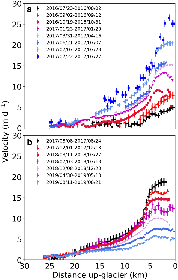
Fig. 8. Centreline surface velocities (metres per day) over Negribreen. (a) Rapidly accelerating velocities during Stage 3, from after the collapse of summer 2016 until melt-season in 2017. (b) Gradual deceleration of velocities during Stage 4 after the melt-season in 2017.
Stage 4, Post-collapse: deceleration
After the velocity peak detected in the melt-season of 2017, the glacier entered a period of deceleration. At the end of 2017, peak velocities decreased to ~15 m d−1, by the end of 2018 down to ~10 m d−1, and in late summer 2019 down to 5 m d−1 (Fig. 8b). As seen in Figure 7c, this slowdown happened rather gradually. Since velocities are still high early post-collapse and stretching the ice, the glacier surface elevation continued to lower in this stage (Fig. 2). Figures 4g, h show similar crevasse extents in 2018 and 2019 as to 2017, but crevassing had become noticeably more intensified, even spreading to Rembebreen and Akademikarbreen.
Discussion
We have interpreted the recent surge event at Negribreen in four stages. All stages show distinct behaviour, and each stage provided the conditions necessary for the next. In this section, we compare our observations to other observed surges in Svalbard. We discuss in detail the basal friction, geometry change and spread of crevasses, all important processes occurring in Stages 1 and 2 which led towards the final onset of this surge event. To help compare observations of recent surges in Svalbard, Table 3 summarizes our observations for Negribreen as well as a number of recent studies of other glaciers.
Table 3. Summary of observations across a selection of tidewater glacier surges in Svalbard. In each column, ‘yes’ indicates that a particular observation was confirmed in the literature, ‘no’ indicates it was confirmed to be absent, and ‘–’ indicates it was not reported. For observations of eskers, the survey year(s) are given. Additionally, ‘SV’ = ‘Surface Velocity’, ‘Crev. init.’ = ‘Crevasse Initiation’

a Dowdeswell and others (Reference Dowdeswell, Hamilton and Hagen1991);
b Rolstad and others (Reference Rolstad, Amlien, Hagen and Lundén1997);
c Luckman and others (Reference Luckman, Murray and Strozzi2002);
d Strozzi and others (Reference Strozzi, Luckman, Murray, Wegmüller and Werner2002);
e Mansell and others (Reference Mansell, Luckman and Murray2012);
f Murray and others (Reference Murray, Strozzi, Luckman, Jiskoot and Christakos2003b);
g Murray and others (Reference Murray, Luckman, Strozzi and Nuttall2003a);
h Murray and others (Reference Murray2012);
i Dowdeswell and Benham (Reference Dowdeswell and Benham2003);
j Fleming and others (Reference Fleming2013);
k Flink and others (Reference Flink2015);
l Sevestre and others (Reference Sevestre2018);
m Sund and others (Reference Sund, Lauknes and Eiken2014);
n Nuth and others (Reference Nuth2019);
o Dunse and others (Reference Dunse2015);
p Strozzi and others (Reference Strozzi, Kääb and Schellenberger2017);
q Benn and others (Reference Benn2019);
r Ottesen and others (Reference Ottesen, Dowdeswell, Bellec and Bjarnadóttir2017);
s Ottesen and others (Reference Ottesen2008);
t Burton and others (Reference Burton, Dowdeswell, Hogan and Noormets2016).
High basal friction and bulge formation
A critical factor related to the surge at Negribreen is the distribution of friction beneath the glacier. At polythermal glaciers such as Negribreen, basal friction is itself related to both the glacier's thermal regime and the amount of liquid water at the bed of the glacier (i.e. the enthalpy of the glacier; Aschwanden and others, Reference Aschwanden, Bueler, Khroulev and Blatter2012; Sevestre and Benn, Reference Sevestre and Benn2015; Benn and others, Reference Benn, Fowler, Hewitt and Sevestre2019), as well as the properties of the bed itself. Persistent, long-term high friction at Negribreen is suggested by the presence of immobile ice near the terminus and the subsequent ‘bulge’ formation (Fig. 2), as well as the presence of eskers in the fjord in front of Negribreen indicating a long-established efficient drainage system. Similar observations of areas with high basal friction and stagnant ice near the terminus have been noted for other surge-type tidewater glaciers in the region, such as for the NGS (Nuth and others, Reference Nuth2019), Basin-3 of Austfonna (Dunse and others, Reference Dunse2015), Stonebreen (Strozzi and others, Reference Strozzi, Kääb and Schellenberger2017) and Perseibreen (Dowdeswell and Benham, Reference Dowdeswell and Benham2003).
On Svalbard, influence of the thermal regime on surge-type glaciers varies according to size and whether they terminate on land or in water, with tidewater glaciers having predominantly temperate conditions at their beds (Sevestre and others, Reference Sevestre, Benn, Hulton and Bælum2015). The observation of a cold-temperate transition surface along the centreline of Negribreen by Dowdeswell and others (Reference Dowdeswell, Drewry, Liestøl and Orheim1984) suggests that the zone of high friction was not due to the thermal regime alone; that is, it is unlikely that the entire terminus region was frozen to the bed. Nuth and others (Reference Nuth2019) showed, with a thermo-mechanical model, that it is sufficient to have localized cold patches at the bed. These cold patches would then act to reduce mean basal sliding, which eventually stabilizes an efficient drainage system through large channels in the sediments, promoting higher friction. This interpretation, which we hypothesize was also the case at Negribreen during Stage 1, is further supported by the observed submarine eskers in the fjord.
Eskers are also found in association with non-surging glaciers and are thus not thought to be diagnostic of surge activity (Dowdeswell and Ottesen, Reference Dowdeswell and Ottesen2016). As all proposed theories of surge behaviour require an inefficient subglacial hydrological system during the active phase of a surge cycle, the eskers are likely to have formed after a surge termination or during quiescence (Ottesen and others, Reference Ottesen2008). Also, any pre-surge eskers are likely to be erased with the passage of the surge front. This may explain why such depositions are not seen in front of the surge glaciers Blomstrandbreen and Tunabreen, as sea-floor surveys were conducted too soon after their respective surges (Flink and others, Reference Flink2015; Burton and others, Reference Burton, Dowdeswell, Hogan and Noormets2016).
Over time, the zones of high friction near the front served as an impediment to ice as it flowed from the accumulation area, causing a ‘bulge’ to form. The long duration of the thickening signal (pre-1990 to 2010), as well as its relatively low magnitude (<2 m a−1), suggests that the bulge formed as a result of ice steadily flowing down from the accumulation area and building up as it encountered the high friction zone. This is contrasting with ice being ‘pushed’ through the glacier system from a destabilizing reservoir area, which has been observed during land-terminating surges in Svalbard like the 1985–1995 surge event on Bakaninbreen (Murray and others, Reference Murray, Dowdeswell, Drewry and Frearson1998). Besides Negribreen and Bakaninbreen, the only other Svalbard surge events with a well-documented bulge formation are the recent events from NGS (Sund and others, Reference Sund, Lauknes and Eiken2014; Nuth and others, Reference Nuth2019) and Moršnevbreen (Benn and others, Reference Benn2019). In other remote-sensing analyses of Svalbard glacier surges, including on Osbornebreen (Rolstad and others, Reference Rolstad, Amlien, Hagen and Lundén1997), Perseibreen (Dowdeswell and Benham, Reference Dowdeswell and Benham2003), Tunabreen (Flink and others, Reference Flink2015), Monacobreen (Luckman and others, Reference Luckman, Murray and Strozzi2002; Murray and others, Reference Murray, Strozzi, Luckman, Jiskoot and Christakos2003b) and Fridtjovbreen (Murray and others, Reference Murray, Luckman, Strozzi and Nuttall2003a, Reference Murray2012), examination of crevasse patterns or DEM differencing shows the absence of a surge bulge travelling down-glacier, which does not necessarily preclude a bulge presence like the one observed on Negribreen.
Furthermore, the extent of the bulge gives information about the footprint of areas with enhanced subglacial friction. In the case of Negribreen, this footprint was stable since at least 1990 as the bulge front did not change its extent before it broke up during Stage 2. This contrasts to one of the bulges from the NGS surge and the bulge on Moršnevbreen, which were reported to migrate down-glacier, indicating a dynamic sub-glacial footprint.
Bulge weakening and collapse
During Stage 2, the bulge weakened, leading to the activation of the surge and the onset of collapse. DEM differencing between 2010 and 2013 (Fig. 2b) shows strong thinning in the terminus region, in the same areas where we observed crevasses in 2004 and 2009 (Fig. 4), and where velocities first began to increase in 2014 and 2015. It is also where we first observe seasonal fluctuations in the glacier length, beginning in 2013. These different lines of evidence strongly suggest that the zones of high friction were shrinking/disappearing.
Between 1990 and 2010, the growth of the bulge led to an increase in surface slope, with the largest increase occurring near the bulge front. Surface steepening at the glacier front is a common observation before a tidewater surge in Svalbard, and it is known to cause increased driving stresses, as observed prior to the respective surges of Aavatsmarkbreen, Nathorstbreen and Stonebreen (Strozzi and others, Reference Strozzi, Kääb and Schellenberger2017; Sevestre and others, Reference Sevestre2018; Nuth and others, Reference Nuth2019). This increase in surface slope led to an increase in driving stress from 58 to 73 kPa, a 1.25-fold increase. Because the basal melt rate is proportional to $\tau _d^4$ (e.g. van der Veen, Reference van der Veen2013), this increase would lead to a 2.4-fold increase in basal melt rate. Between 2010 and 2015, the driving stress increased slightly from 73 to 79 kPa, which would lead to a further 1.6-fold increase in basal melt rate. This increase in melt rate could have led to a reduction in basal friction near the terminus, encouraging an increase in velocity. While the increase in basal melt rate was likely not the sole cause of the destabilization, the decrease in basal friction and subsequent increase in surface velocities observed could have started a feedback cycle that eventually led to the collapse.
Ocean forcing has been shown to be able to influence rates of frontal ablation (submarine melt + calving; e.g. Motyka and others, Reference Motyka, Hunter, Echelmeyer and Connor2003; Bartholomaus and others, Reference Bartholomaus, Larsen and O'Neel2013) at several tidewater glaciers in Svalbard (Luckman and others, Reference Luckman2015). In that study, Luckman and others (Reference Luckman2015) argued that the observed strong correlation between frontal ablation rate and ocean temperature indicated melt-driven convection at the ice-ocean interface, which is highly sensitive to ambient ocean temperatures (Jenkins, Reference Jenkins2011). During Stage 1, Negribreen was retreating into deeper water (Ottesen and others, Reference Ottesen, Dowdeswell, Bellec and Bjarnadóttir2017), exposing more of the glacier terminus to submarine melt throughout the year, which could have aided in its destabilization. However, Negribreen outlets on the eastern coast of Svalbard, where ocean temperatures are typically lower than on the west coast (Jakowczyk and Stramska, Reference Jakowczyk and Stramska2014), suggesting that the influence of the ocean may not be as strong as at other glaciers. We also do not see any strong correlation between ocean surface temperatures and either length change or surface velocity, further suggesting a smaller influence of the ocean in this case.
Another external influence could come from sea-ice conditions, which have been shown to influence calving rates, glacier dynamics and terminus stability in other regions like Greenland (e.g. Joughin and others, Reference Joughin2008; Amundson and others, Reference Amundson2010) and Novaya Zemlya (Carr and others, Reference Carr, Stokes and Vieli2014). However, despite a reduction of sea ice from 2000 to 2010, the true significance of this might be negligible in Stage 1, as ice near the terminus is mostly immobile, and no clear signals are seen in length changes. Potentially, there could be higher sea-ice influence in Stage 2, when the glacier front becomes mobile, but to what degree is difficult to speculate based on the available data.
Dating to the 1990s, we observe small zones of crevasses near the terminus of Negribreen. During Stage 1, there are few signs of expansion of these zones, which tend to occur near or overtop areas of assumed efficient subglacial channels, observed as submarine eskers. As none of our observations suggest increased dynamics during Stage 1, it seems likely that these crevasses were not deep enough to influence the bed of the glacier via input of surface meltwater. However, this seems to have been the case in Stage 2. The up-glacier expansion of the crevassed regions correlates well with both the strong thinning and increase in surface velocity. This points towards a positive feedback cycle where increasing velocities feed the appearance of crevasses, leading to more surface water lubricating the bed, further allowing velocities to increase. This feedback cycle was observed on both Basin-3 of Austfonna (Dunse and others, Reference Dunse2015) and Stonebreen (Strozzi and others, Reference Strozzi, Kääb and Schellenberger2017) during their pre-surge acceleration. On Basin-3, high temporal resolution Global Positioning System (GPS) measurements showed that the at least 4-year long multi-annual acceleration was not gradual, but occurred in steps, each following a summer speedup. A similar trend can be seen in Figure 7c, where Negribreen between at least two successive summers had detectable step increases in velocity, though the detail of documentation during this period is not as high as on Basin-3. Surface melt-water input to the bed would provide an increase in enthalpy, as it is both an efficient heat source and a source of liquid water. The warming caused by this meltwater input would help to remove any remaining cold patches at the bed causing high friction, and together with frictional heating from deformation, would further enhance sliding and promote increased crevassing at the glacier surface.
Conclusion
We have investigated the ongoing surge of Negribreen, a tidewater glacier on the east coast of Svalbard. From remotely sensed data with high temporal resolution, we have shown that this surge of a tidewater glacier is composed of four distinct stages. The initiation of the active surge itself occurred after a long-term geometric change and frontal destabilization in Stages 1 and 2, respectively. We find that the ‘onset’ of the surge is a chain of connected processes, which began in Stage 1 with the establishment of high friction beneath the lower portion of the glacier. Our interpretation is that the zone of enhanced friction was a combination of cold patches of ice as well as an established efficient subglacial drainage system, indicated by eskers imprinted on the seafloor in front of the glacier. Consequently, the high-friction barrier divided the glacier flow regime into an immobile zone at the front and a mobile zone further up-glacier. This caused a gradual modification of the glacier geometry with the development of a bulge at the high-friction boundary, increasing of surface slope at the bulge head, and thinning of the glacier front.
The frontal thinning is a very important process in the feedback proposed here. First, it lowered a potential driving-stress threshold by increasing the surface slope, which eventually decreased the subglacial friction and promoted a rapid frontal destabilization through increasing basal lubrication by surface melt-water through enhanced crevassing. This in turn caused accelerating thinning rates due to rapidly accelerating surface velocities. A pattern of up-glacier propagating crevassing, initiated at the terminus, shows similar dynamic evolution as has been documented on other surging tidewater glaciers in Svalbard. Our study demonstrates how a combination of the wealth of remotely-sensed data currently available enables us to decipher surge evolutions in an unprecedented way, and to newly interpret past events with less comprehensive data coverage.
Acknowledgments
This research has been supported by the European Research Council (project: FP/2007-2013/ERC; grant no. 320816) and the European Space Agency Glaciers-CCI, CCI+, ICEFLOW, and EE10 HARMONY projects (4000109873/14/I-NB, 4000127593/19/I/NB, 4000125560/18/I-NS, 4000127656/19/NL/FF/gp). Additional support was provided by the Norwegian Space Centre project Copernicus Glacier Service for Norway (NIT.06.15.5). The study is a contribution to the Svalbard Integrated Arctic Earth Observing System SIOS. Radarsat data were provided by NSC/KSAT under the Norwegian-Canadian Radarsat agreements 2007–2019. ERS-1/2 data were provided by ESA through PRODEX. TanDEM-X DEM was provided through DLR grant IDEM GLAC0435. We are very grateful to USGS for Landsat data, and the Norwegian Polar Institute for the historical map data/DEMs. Acquisition of ASTER images was guided by NASA JPL through the ASTER science team and the Global Land Ice Measurements from Space (GLIMS) initiative. ArcticDEM DEMs provided by the Polar Geospatial Center under NSF-OPP awards 1043681, 1559691 and 1542736. We thank the GoLIVE project for providing free velocity data for the public. We also thank Scientific Editor Hester Jiskoot and two anonymous reviewers for their constructive comments which helped improve the clarity of the manuscript.


 Open access