


1. Introduction
The response of a glacier to changes in the rate of accumulation and ablation bas been examined theoretically in previous papers (Reference NyeNye, 1960, Reference Nye1963[a], Reference Nye1963[b], ) which will be referred to as Nye [I], Nye [II] and Nye [III]. In this paper we use exactly the same differential equations as before and present new numerical results for the frequency response of (a) an artificial glacier chosen for analytical simplicity, (b) South Cascade Glacier, Washington, U.S.A., and (c) Storglaciären, Kebnekaise, Sweden.
Let us first recall the assumptions of the theory and the basic equations. The assumptions are that (a) the ice has constant and uniform density, (b) the discharge q through a cross-section at x, where x is distance measured down the glacier, is a function of x, the thickness h of the glacier at that section, and the slope a of the upper surface at that section. Thus
h could be taken, for convenience, as the maximum thickness at the section. By this assumption we postulate that any change of discharge at given x is produced only by a change in the thickness or surface slope of the glacier at the cross-section in question. The theory cannot therefore take account of changes in discharge caused by changes in ice temperature, which will change the flow law; nor can it take account of changes in ice discharge caused by physical changes at the ice-rock interface, as might be caused, for example, by an increase in the amount of lubrication by melt water.
Under a steady rate of accumulation and ablation a 0(x), the glacier will reach a steady state, called the datum state. a 0(x) is positive for accumulation and negative for ablation and is measured as thickness of ice per unit time. The theory is concerned with the behaviour of small perturbations from this datum state. The equations for the perturbations are

q 1(x, t), h 1(x, t) and a 1(x, t) are the perturbations of the discharge, thickness and accumulation-rate from the steady-state values. B 0(x) is the width of the upper surface of the glacier, and is supposed not to change during the perturbation. c 0(x) and D 0(x) are functions which, like B 0(x), characterize the particular glacier under consideration; c 0/B 0 has the physical interpretation of a kinematic wave velocity while D 0/B 0 is a diffusion coefficient. The details of the derivation of equations (1) and (2) are given in Nye [III]. If B 0(x), c 0(x), D 0(x) are known functions, (1) and (2) are two simultaneous linear equations for determining the q 1(x, t) and the h 1(x, t) which result from a given perturbation a 1(x, t) in the rate of accumulation and ablation. It is a simplification to assume that a 1(x, t) is independent of x, so that we may write it as. A more general assumption about the x dependence is that
where X(x) is a known function. But although all the computer programmes to be discussed have been written for a general function X(x) it has in fact proved adequate in all applications so far to take X(x) ≡ 1. We shall therefore make this simplification throughout and write a 1(x, t) = a 1(t).
In this paper we are concerned with the response of a glacier to a simple harmonic variation of a 1(x, t). Thus we put
where A is real. Since the system is linear the response, after transients have disappeared, will be harmonic variations of h 1(x, t) and q 1(x, t) of the same angular frequency w but, in general, different phase. Thus we write
where H and Q are complex. H and Q are the complex amplitudes of the response at given x to an applied signal of uniform amplitude A and angular frequency ω. Substitution in equations (1) and (2) gives

As already stated, B 0, c 0, D 0 are known functions of x, and A is a real constant. These two equations then give the complex functions H(x) and Q(x) for a given choice of ω. Since Q and H are directly proportional to A, A may be taken equal to 1 without loss of generality. Q and H are then the response amplitudes to a unit-amplitude oscillation of a 1
2. Direct Computation of Response Curves
The above introduction simply summarizes the relevant parts of Nye [III] without adding anything new.
In Nye [II] equations (3) and (4) were considered for a special model in which the functions characterizing the glacier have the simple polynomial forms

where σ, δ, E, l are positive constants. σ is a time, δ is dimensionless and much less than 1, E is dimensionless, and l is related to the length L of the glacier in the datum state by l(1−δ) = L. The glacier in the datum state runs from x = 0 to x = L. A solution in closed form was found for E = 1.
In a real glacier one wishes to solve (3) and (4) when B 0(x), c 0(x), D 0(x) are given graphically. In Nye [III] this was done by obtaining series approximations of the form

and

valid for low frequencies, and

valid for high frequencies. A scheme for computing the λ’s and ν’s from known functions B 0(x), c 0(x), D 0(x) was developed and applied to data derived from Dr. Mark F. Meier’s work on South Cascade Glacier, Washington, U.S.A. In this way the frequency response of South Cascade Glacier was computed. The work was done on a desk calculator.
When automatic digital computers became available to the author two possibilities presented themselves. First, to write a programme for the calculation of μ and λ coefficients previously done by hand, which could then be used for data on any glacier. The results from this programme will be described later. Second, instead of obtaining the frequency response in two stages, by first computing the λ’s and v’s and then using the two series (7) and (8), it should be possible to compute solutions of (3) and (4) directly for a number of different wg’s, thereby finding the response curves. This would be a more direct way of finding the frequency response, and at the same time would avoid any difficulties in the intermediate range of frequencies where both (7) and (8) might break down.
(i) Results for analytical model
As a start I investigated solutions of (3) and (4) with B 0, c 0, D 0 having the special forms (5). σ is taken as the unit of time and l as the unit of length. A is also put equal to 1 without loss of generality since both Q and H are directly proportional to A. The equations are then

with

and with the datum glacier running from x = 0 to L, whereL = 1−δ. Thus 0 ≤ x ≤ L < 1.
The boundary conditions at x = 0 and x = L need special consideration. D 0 = 0 at both end points, which are regular singularities of the equations. The problem is fully discussed in Appendix I (see also Nye [II]) and here we need only quote certain results. A unique solution for any given w is determined if we simply require that H be not infinite at x = 0 or x = L The requirement at x = 0 is equivalent to putting Q = 0 at this point. Near x = 0 there is a one-parameter family of solutions satisfying the boundary condition, in the sense that a particular solution is fixed by the value of one complex constant; but the leading term is the same for all members of the family, namely

where the dots stand for terms of higher order in x.
Near x = L there is also a one-complex-parameter family of solutions satisfying the boundary condition. The leading term in this family of solutions, when they are expanded about the point x = L, is an arbitrary complex constant. For all this family of solutions, at x = L,
and

where the primes denote differentiation with respect to x. (14) is derived by putting D 0 H′ = 0 in (10) (more strictly in (14)); the second may be obtained by differentiating (10), putting D 0 H″ = 0, and substituting for Q′ from (9). The jusgification for putting D 0 H′ = 0 and D 0 H″ = 0 at x = L is that D 0(L) = 0 and, as shown in Appendix 1, H′(L) and H″(L) are not infinite in the family of solutions satisfying the boundary condition.
The method of solution is to integrate the simultaneous equations backwards from x = L, using (9) and (10) at all points except x = L; at x = L (10) does not suffice to fix H′ because D 0 is zero; we therefore use (15) instead. The starting values of H and 0 are not known, and must be chosen by trial so that the solution satisfies the boundary condition at x = 0, that is, so that Q = 0 or H is not infinite. To avoid the trial solutions becoming infinite the testing is done not at x = 0 but at x = ϵ, ϵ being small. The value we have to achieve is
from (13). The trials are made as follows. Write H = u+iv and Q = r+is where u, v, r, s are real. Choose arbitrary starting values for u, v, say (0, 0), at x = L. Find r , s from (14). Then integrate back to x = ϵ. Let the resulting values of r, s at x = ϵ be r 1, s 1. Now choose a new pair of starting values for u, v, say (1, 0), and repeat the integration, obtaining at x = ϵ the values r 2, s 2. Since Q(ϵ) depends linearly on the starting value H(L) we have, in general,
or, taking real and imaginary parts,
and
where j = j 1+ij 2 and k = k 1+ik 2 are complex constants. j 1, j 2, k 1, k 2 are fixed by the definitions of r 1, s 1 and r 2, s 2 so that we have
Thus the constants in the linear relation are determined by the known values r 1, r 2, s 1, s 2. If r(ϵ) and s(ϵ) are now assigned the values required by (16), (17) and (18) may be solved to give the correct starting values u(L), v(L). A final integration is now performed using these starting values, and it should strike the target values r(ϵ), s(ϵ) required by (16). This is the required solution.
This methodFootnote * was programmed for an I.B.M. 709 digital computer, using a Runge-Kutta integration method, with ω, E, δ and ϵ as variable parameters. It worked successfully for values of ω from 0 to about 30 (with δ = 0.01), and was checked against the known analytical solution for E = 1. The precision was checked by changing ϵ and the interval. At the highest frequencies ω ≥ 18 the fit with the boundary condition at x = ϵ deteriorated. This is because, at these frequencies, a very small change in the starting values at x = L has a large effect at x = ϵ (or, put the other way round, a large input Q at x = 0 would be needed to produce a sensible effect at x = L, because of attenuation by diffusion); thus for a reasonable fit at x = ϵ very many significant figures would be needed in the starting values at x = L. But this effect need not trouble us, because the main purpose was to find the response at x = L, and this is still determined quite precisely even though the fit at x = ϵ is bad. At still higher frequencies (say ω > 50), where overflow may occur in the trial integrations, the result is best obtained by using the high-frequency series (8), of which the leading term is simply H(x)/A = (iω)−1.
The results at x = L for E = 0.1 and 1 are shown in Figures 1a, b, c, d. (Results for E = 2 did not differ much from those for E = 1.) If we look first at the curve for E = 1 in Figure 1a (already known from Nye [III), the amplitude |H| of the response to unit amplitude A approaches the value δ = 100 at low frequencies, and approaches zero as ω −1 at high frequencies. On the plot of log |H|: log ω in Figure 1b the curve for E = 1 is below the straight line |H|−ω −1 (broken line) at low frequencies, above it at medium frequencies, and approaches it asymptotically at high frequencies. This may be explained by saying that at high frequencies the glacier acts as a perfect integrator of the changes in accumulation rate, that is ∂ h1/∂t = a 1, giving the response |H| ~ ω −1. At medium frequencies the response at the terminus is greater than this because it is reinforced by kinematic waves from higher up the glacier. But at low frequencies the glacier no longer integrates, because the leakage rate is too fast, and we have h 1 simply proportional to a 1

Fig. 1a. Frequency response at the terminus of an artificial glacier. The response amplitude |H| to a unit amplitude variation of accumulation and ablation rate is plotted against angular frequency ω. ω is measured in natural units (σ = 1). For illustration a scale of periods, taking σ = 6 yr., is shown at the top

Fig. 1b. Same as Figure 1a, but showing |H| on a logarithmic scale

Fig. 1c. Same as Figure 1a, but showing the phase lag ϕ of H on A

Fig. 1d. Frequency response at the terminus of an artificial glacier, with E = 0.1. A polar plot of the end of the vector H as ω changes. Numbers against the curve are values of ω in natural units (σ = 1)
The curves of |H| for E = 0.1 in Figures 1a, b are similar in general form to those for E = 1, but they cross at ω = 1.2 (owing presumably to more destructive interference between the waves).
The phase lag ϕ of the response at x = L, defined by
is plotted against log ω in Figure 1c. The curve for E = 1 goes through a maximum (at
It seemed desirable for completeness to calculate the response for E = 0, which corresponds to no diffusion and therefore pure kinematic wave propagation down the glacier. The differential equations become of first order and hyperbolic, instead of second order and parabolic. The numerical method used for non-zero E fails for this case. It is shown in Appendix II that, if B 0(x) ≡ 1 and D 0(x) ≡ 0, the response at x = L may be expressed quite generally as

where

T(ξ) is the travel time for a wave from x = ξ to x = L; in the case under consideration where c o is given by (11)

The integral in (19) was evaluated numerically. At small ξ, ωT(ξ) in the integrand is large and rapidly changing, so the integral was approximated in the range ξ = 0 to ϵ by the first two terms in the power series in ϵ. Over the rest of the range ξ = ϵ to L, Simpson’s Rule was used. With ϵ between 10−5 and 10−2, and with the remainder of the range divided into 400 intervals, this procedure was satisfactory for values of ω up to about 2. The accuracy was checked by changing ϵ and the interval.
For ω > 2 a very small interval would have been needed near ξ = ϵ to cope with the rapid change of ωT. It seemed preferable to deal with this range of ω by direct integration of the original differential equations. At the same time this gave a check on the previous results. Equation (4) simply reduces to Q = c 0(x)H, with c 0(x) = x(1−x), and equation (3) therefore becomes

The boundary condition is Q = 0 at x = 0. At x = 0, which is a singularity, (21) does not suffice to determine Q′ directly. In the neighbourhood of x = 0 the equation is sufficiently well represented by
which has the general solution

where P is an arbitrary constant. P = 0 by the boundary condition, and hence

(21) and (22) were integrated from x = 0 to L (L = 1−δ, δ = 0.01) by a Runge-Kutta method. The previous results from (19) were checked and the range of ω extended up to ω = 5.6 (where the ranges 0 ≤ x ≤ 0.891 and 0.891 ≤ x ≤ 0.99 were divided into 540 and 600 intervals respectively).
The results for E = 0 are seen in Figures 1a, b, c, e, f. Figure 1a shows |H|:log ω. The drop from maximum response takes place in a rather narrower frequency band when there is no diffusion. In Figure 1b, which shows log IHI: log w, the response amplitude is seen to oscillate before settling down to fall off as ω −1. The phase lag ϕ, is no longer confined within a single 360° range. This is seen in the polar plot of Figures 1e, f; as w rises from 0 to 2.95 the vector H rotates clockwise through


Fig. 1e. Same as Figure 1d but for E = 0

Fig. 1f. Region near the origin of Figure 1e
for δ = 0.01. This gives values of ϕ correct to about 1 per cent up to ω = 2.
A polar plot of H, such as Figures 1d, e, f, must start at ϕ = 0 and finish at ϕ = 90°. For E = 0.1 it does not encircle the origin (Figure 1d), but for E = 0, as we have seen, it encircles the origin twice. This poses a continuity problem. As E changes continuously between 0 and 0.1 the curve must change the number of times it encircles the origin first from 2 to 1 and then from 1 to 0. How it can do this in a continuous fashion is an interesting question which has not been studied in detail. Probably, for certain small values of E, the curve actually traverses the origin for finite ω. This would mean that H = 0 for certain finite w—with an infinite downward oscillation on a plot of log |H|: ω. The terminus would be a node for these frequencies.
(ii) Results for South Cascade Glacier
Having studied the numerical solution of the basic equations (3) and (4) with B 0, c 0 and D 0 having the special forms (5), it was a simple matter to modify the computer programme described in §2(i) so that B 0, c 0 and D 0 could be specified in numerical form rather than calculated algebraically. The behaviour of B 0, c 0, D 0 at the end points is restricted to the forms given in Appendix I: namely that, near x = 0, B 0(x) ~ constant, c 0(x) ~ x, D 0(x) ~ x 2, and near x = L, B 0(x) ~ constant, c 0(x) ~ constant, D 0(x) ~ L−x. The physical jusgification for this choice of behaviour at the end points is discussed in Nye [II] and [III]. The resulting programme was first checked by computing the frequency response of South Cascade Glacier (Reference Meier and TangbornMeier and Tangborn, 1965), which was already known from previous work [Nye III] using the series approximations (7) and (8). The input data on B 0, c o, D 0. were identical to those used for the earlier hand calculation, except for a slight change to make B 0 non-zero at x = 0 which ought to have been made before. The resulting frequency response curves are shown in Figures 2a and b. The curves computed earlier, and reported in Nye [III], are also shown for comparison. In the parts of the curves previously obtained by the low frequency series (7) there is no significant difference. But there are significant differences in the ϕ curves near the maximum. It seems that the earlier results using the ν series (8) were less accurate for ω < 0.6 yr−1. than was thought at the time, and that the useful range of this series is therefore rather small. There is a suggestion of an oscillation in ϕ near ω = 2 yr−1, which is presumably a real effect in view of the similar oscillation seen in the special model for E = 0.1 and o. The direct computation of H by solving the equations for fixed w is certainly a much better procedure when an automatic computer is available.

Fig. 2a. Frequency response at the termini of two glaciers. The response amplitude |H| to a unit amplitude variation of accumulation and ablation rate is plotted against angular frequency ω, and the period (top scale). Scale on center: Storglacidren. Scale on right: South Cascade Glacier. Light broken curve shows results of previous calculation on South Cascade Glacier

Fig. 2b. Frequency response at the termini of two glaciers. The phase lag ϕ of H on.A is plotted against angular frequency ω and the period (top scale). Broken curve shows result of previous calculation on South Cascade Glacier
We next wished to use the same computer programme to find the frequency response of Storglaciären, Kebnekaise, Sweden. The first step, namely the deduction of the functions B 0(x), c 0(x), D 0(x) from observation is described in the next section. The method used is very similar to that described in Nye [III] for South Cascade Glacier.
3.B0(x), c 0(x) and D 0(x) for Storglaciären
Storglaciären, a valley glacier with an area of 3.1 km.2, situated in the Kebnekaise massif of northern Sweden, has been studied since 1945 (Reference SchyttSchytt, 1959, Reference Schytt1962) with a view to relating budget and climate. The earliest measurement of the terminus position was made in 1897. Professor H. W:son Ahlmann and Dr. V. Schytt have generously made the measurements, both published and unpublished, available to me for the present study. The material used has been:
-
i. a topographical map of the glacier for 1959 (prepared at Rikets Almänna Kartverk under the supervision of Dr. Erik Woxnerud);
-
ii. curves of accumulation and ablation as a function of altitude for all budget years from 1945–46 to 1961–62 (the data from 1949–50 to 1958–59 were collected and reduced by Dr. Woxnerud);
-
iii. a long profile of the glacier surface and bed (seismic work by S. R. Ekman);
-
iv. data on surface velocities (supplied by Dr. Woxnerud).
An x-axis was set down the line of the measured profile. The breadth B(x) was read from the map and taken as B 0(x) (Fig. 4), except for the snout region. The theoretical model requires that the glacier have a wedge-shaped snout, with B 0(x) non-zero at the terminus. Therefore a terminus of this type was arbitrarily constructed as the datum state, having an area roughly equal to the real area in 1959. This gave L = 3, 300 m.
A curve of mean elevation as a function of x was constructed from the contour map and used to plot curves of net budget (equal to accumulation minus ablation) versus x (Fig. 3). The mean of these net budget curves for 1946–61 was then displaced upwards (by 65.1 cm. of ice/yr.) so that the resulting curve a 0(x) made the integral


Fig. 3. Net budget of Storgiaciaren, from 1945 to 1962 plotted against distance x down the glacier. Numbers on curves refer to budget year, e.g. 46 means 1945–46. Curves are derived from observations provided by Prof. H. W:son Ahlmann, Dr. V. Schytt and Dr. E. Woxnerud

Fig. 4. Measured width B(x) and datum width B0(x) for Storglaciären. B(x) is from data provided by Prof. H. W:son: ihlmant, Dr. V. Schytt and Dr. E. Woxnernd
Having fixed a 0(x), the datum-state discharge q 0(x) was computed from

The datum-state surface slope a 0(x) was taken from the curve of mean current elevation versus x. Hence D 0(x) was computed from the formula
derived in Nye [III].
If the glacier is assumed to have a parabolic cross-section the average velocity u 0(x) through a section in the datum state is related to the discharge q 0(x) by
where h 0(x) is the maximum depth. h 0(x) was assumed equal to the measured depth. Hence u 0(x) was found. The values of u 0(x) were found to be not significantly different from the velocities directly measured on the surface centre-line. Thus, by a coincidence, if the velocity of the glacier were to increase so that the mean velocity over a section was equal to the current centre-line velocity, the glacier would reach a steady state at its current length. Having found u 0(x), c 0(x) was deduced from the formulae

derived in Nye [III].
The resulting functions c o (x), D 0(x) are shown in Figure 5. In making the functions have the behaviour required by the analysis at the end points no violence is done to the observational data.
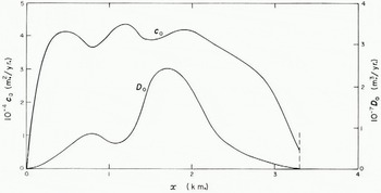
Fig. 5. c 0(x) and D 0(x) for Storglaciären inferred from observation provided by prof. H. W: son Ahlmann, Dr. V. Schytt and Dr. E. Woxnerud
4. Frequency Response of Storglaciären
The same programme that was used for South Cascade Glacier gave the frequency response curves for the snout of Storglaciären shown in Figure 2a and b. The general shapes are the same. The amplitude |H|/A for low frequencies is twice as great as for South Cascade Glacier—586 yr. (meaning 586 cm. for A = 1 cm./yr.) as against 291 yr. for South Cascade Glacier. This is because this amplitude is given by S 0/u 0(L), where S 0 is the area of the datum glacier. The area of Storglaciären (3.1 km.2) is about the same as that of South Cascade Glacier (2.7 km.2), but Storglaciären moves only half as fast. Hence the amplitude is twice as great.
Another feature of interest is the double maximum on the curve of ϕ: log ω, which does not appear for South Cascade Glacier. The centre of this double peak is at ω = 0.115 yr.−1 whereas the peak for South Cascade Glacier appears at ω = 0.240 yr.−1 which is almost exactly twice the frequency. (The periods are 55 yr. and 26 yr. respectively.) The reason is again that Storglaciären has almost the same length and breadth as South Cascade Glacier but moves at only half the speed. All time constants are therefore doubled.
5. μ and λ Coefficients for South Cascade Glacier and Storglaciären
A programme for calculating the μ and λ coefficients in the low frequency series (6) and (7) was written; the method was identical to that previously used with a desk computer, except that the integrations of the differential equations were done by a Runge-Kutta technique instead of by a predictor-corrector method. The programme was first tested on the B 0, c 0, D 0 data for South Cascade Glacier (which were almost identical to those used in the hand calculation). The results for x = L are shown in columns (1) and (2) of Table I, with the previous results shown for comparison in column (3). The dependence of the results on the number of intervals used is an indication of the accuracy. The interval could have been further reduced, but in view of the uncertainty in the starting data on B 0, c 0, D 0 any greater precision obtained would be illusory. The agreement with the result of the hand calculation is reasonable.
The same programme used with the B 0, c 0, D 0 data for Storglaciären gave the results shown in columns (4) and (5) of the table. The μ’s for Storglaciären are all greater than those for South Cascade Glacier, again because Storglaciären moves relatively slowly. (The λ’s also follow this pattern, less obviously: those with positive time dimensions are greater, while λ 0, with dimensions time−1, is less.)
Table I Values of μ’s and λ’s at x = L

6. Conclusions
The method for finding the frequency response of a glacier described in §2, by direct solution of the equations for given ω, is much superior to the earlier method which used high and low frequency approximations. Unlike the earlier method it needs an automatic digital computer. (An analogue computer might also be very suitable but I have not studied this possibility.) The method makes it possible to see rather clearly the effect of varying the amount of diffusion of the kinematic waves in the special analytical model (Figs. 1a, b, c, d, e, f).
The frequency response of South Cascade Glacier obtained by this means (Figs. 2a, b) verifies the earlier calculation made with the low frequency series; but it shows that the earlier results for high frequencies need correction. The response of Storglaciären, Kebnekaise, is found to be qualitatively very similar to that for South Cascade Glacier but the time scale is changed by a factor of about two; Storglaciztren moves more slowly and response times are twice as long. The phase of the response of Storglaciären shows a double peak which does not apparently occur for South Cascade Glacier.
The μ and λ coefficients for Storglaciären also reflect the slower time scale for this glacier.
7. Acknowledgements
My sincere thanks are due to Prof. H. W: son Ahlmann, Dr. V. Schytt and Dr. E. Woxnerud for providing me with unpublished material gathered since 1945 in their extensive study of the regime of Storglaciären. I should also like to thank Dr. M. H. Rogers of Bristol University for suggesting the basis of the numerical method used to integrate equations (3) and (4). The first trial computations were run on the I.B.M. 1620 digital computer at Bristol University, and all later computations were done on the I.B.M. 709 digital computer at the Computer Center, Yale University.
Appendix I
Behaviour of the Basic Equations Near the End Points
We consider the equations
where the primes denote differentiation with respect to x; B 0(x), c 0(x), D 0(x) are known functions, W(x) is a known (real) driving function, and it is required to solve for the unknown functions Q(x), H(x) in the range x = 0 to x = L. ν is a parameter that may be positive real, pure imaginary, or zero. Equations (3) and (4) in the main part of the paper have this form if we write v = iω and W(x) = B 0(x) A. The equations are written in the more general form (23) and (24), where v can be real as well as imaginary, so that the following discussion shall be applicable to the similar equations used in deducing influence coefficients in the following paper [Nye V].
(i)The homogeneous equations. Near x = 0. ν real and ≥ o
Here we consider the complementary function which is the solution of the homogeneous equations formed by putting W(x) = 0. Thus
Let the behaviour of the coefficient functions near x = 0 be:

This behaviour includes both the special model of equations (5) in the text, and also the two applications to real glaciers. For a solution near x = 0 put
Substitute in (26) to find Q, then substitute in (25) and equate coefficients of x s to obtain the indicial equation
of which the solutions are
Since c 1, d 1, B 1 are all positive and ν ≥ o, the roots are real and opposite in sign. Let them be s 1 (positive) and s 2 (negative).
The leading terms of the two linearly independent solutions are proportional to x s1 and x s2 respectively. (This is true even in the exceptional case where s 1 and s 2 differ by an integer (see e.g. Reference Morse and FeshbachMorse and Feshbach, 1953, p. 532–33).) Therefore one of the two independent solutions for H is infinite at x = 0. a 1, a 2, .., can be expressed as multiples of a 0 by equating coefficients of higher powers of x. Hence there is a one-parameter set of solutions H(x) satisfying a boundary condition that H(x) is not infinite at. x = 0. This is the first result we wish to establish.
We now show that this boundary condition is equivalent to Q = 0 at x = 0. We have, by substitution of (27) in (26)
Hence, since s 1>0, the solution containing s 1 gives Q(x) = 0. Now, from (28),

that is
the equality occurring if ν = 0. Therefore in the solution containing s 1 the exponent of the first term in (29) is negative or zero. The coefficient (c 1−sd 1) a 0 is never zero. So the solution containing s 2 gives Q(0) infinite if ν > 0, and Q(0) finite and non-zero if ν = 0. Hence the condition Q(0) = 0 is equivalent to the condition H(0) not infinite.
(ii) The inhomogeneous equations. Near x = 0. ν real and ≥ 0
Near x = o let
where the dots stand for terms in x of higher order than zero. We have to find any particular integral of equations (23) and (24). For this purpose try
Substitute in (24) to find Q, then substitute in (23) and equate the constant terms to give
The leading terms in the general solution are thus
where s 1 > 0, s 2 ≤ −1, and a 0 and b 0 are arbitrary constants. The boundary condition H(0) not infinite necessitates b 0 = b 1 = 0. It is important to notice that, after the leading constant term W 1/(c 1+νB 1) from the particular integral, the next term may either be from the particular integral or may be the term a 0 x s1 from the complementary function. For example, if ν = 0, s 1 = c 1/d 1, and with the special forms (11) and (12) used in the paper this gives s 1 = 1/E(1−δ). If E = 0.1, s 1 is about 10 and so in this case the complementary function does not appear until about the term x 10.
The behaviour of Q(x) is found from (24) as:

Thus again the condition Q(0) = 0 is equivalent to the condition H(0) not infinite.
For all the members of the one-parameter family of solutions satisfying the boundary condition at x = 0 the leading term is the same, namely

This is the second result we wanted to establish.
(iii) Near x = 0. ν = iω
This case with ν pure imaginary (ω real) is the one needed for the present paper. The analysis proceeds exactly as before except that Q(x) and H(x) are now complex.
The indicial equation solves to give
Let the roots, which are now complex, be s 1 = u 1+iv 1 and s 2 = u 2+iv 2 The leading terms in |H(x)| for the two independent solutions are
(iv) The homogeneous equations. Near x = L
Put y = L−x, and let the behaviour of the coefficient functions be

Equations (23) and (24) become

where the primes now denote differentiation with respect to y. Put W(y) = 0, and for a solution near y = 0 put
If ν = iω the coefficients a 0, a 1, .., will be complex. Substitute into the equations, as before. The lowest power of y is y s−1, giving the indicial equation
whose roots are s = 0 or s = −c 1/d 1. The general solution then has the leading terms
The subsequent coefficients in the two power series are proportional to a 0 and b 0 respectively, so that there is a two-parameter set of solutions. If ν = iω the two parameters will be complex.
(v) The inhomogeneous equations. Near x = L
Let W(y) = W 1+O(y), and for a particular integral try
By substitution we find, for the leading term,

The higher coefficients H 2, H 3, …, may also be readily determined. The general solution is thus
If we impose the condition |H| not infinite at x = L (y = 0), the second part of the complementary function is eliminated, since the exponent −c 1/d 1 is negative. There is then a one-parameter (a 0) set of solutions in the neighbourhood of x = L satisfying this boundary condition. (We remember that if ν = iω this parameter is complex.) Note that, at x = L, unlike the situation at x = 0, the leading term in these solutions is an arbitrary constant, a 0. Note also the result used in the text that for these solutions H′ and H″ at x = L are not infinite.
Appendix II
Frequency Response with no Diffusion
We derive here some results for the frequency response of a glacier in which diffusion is neglected. Earlier work on this problem is described in Nye [I]. We treat the case B 0(x) ≡ 1 and put D 0(x) ≡ 0. Equations (3) and (4) then reduce to

Substituting for H in the first equation gives the first-order ordinary differential equation for Q:

The integrating factor is most conveniently taken as exp {−iωT(x)} where

T(x) is then the time taken for a kinematic wave travelling with velocity c 0 to go from the point x to the end of the glacier. Multiplying the differential equation by exp {−iωT(x)} and integrating from o to L we have

On the center-hand side Q = 0 at x = 0 by the boundary condition and T(L) = 0 by its definition. Hence we simply obtain

Alternatively, the independent variable in the integrand may be taken as T. From the definition (32),

Since T is a function of x, x may be expressed as a function of T, and hence c 0, originally a function of x, may be expressed as a function of T, namely c 0(T). We then have

where T 0 is the value of T(x) for x = 0.
Equations (33) and (34) are the leading results we want. In (33) the response at x = L is expressed as a sum of contributions from all points up-stream with the appropriate phase delays. In (34) the response is expressed as the sum of a number of contributions of linearly varying phase, each with amplitude c 0(T)dT. (The vector diagram used in optical diffraction problems is analogous. We see, incidentally, that the length of the spiral vector diagram is constant and equal to the length of the glacier, for

A resultant vector of length L corresponds to ω = 0. As ω increases from zero the vector diagram curls up, maintaining constant length, and the resultant decreases in length.) H(L) is readily obtained from Q(L) simply by dividing by c 0(L).
A possible shape for the function c 0(x) is shown in Figure 6a. We have drawn the curve symmetrically about a point x = x m , and have arranged that c 0(0) = 0 and c 0(L) is non-zero. Both the special model used in this paper

Fig. 6.
and the one considered in Nye [I]

have these features. The function c 0(T) then has the general shape, for T > 0, shown in Figure 6b. c 0(T) is non-zero at T = 0, rises to a maximum and then approaches zero as T→∞. Since c 0 = o at x = 0, T 0 is infinite.
If we now arbitrarily define c 0(T) for negative T as zero, equation (34) may be rewritten with new limits of integration as

Thus Q(ω, L) is the complex Fourier transform of c 0(T).
If c 0(x) is symmetrical about its maximum at x = x m , it is readily shown that c 0(T) is also symmetrical about its maximum, at T = T m say, except of course for the missing tail at T < 0. We now derive a standard result for the complex Fourier transform of a symmetrical function. Let f(T) be a function of T symmetrical about T = 0: f(T) = f(−T). Now shift the function f(T) a distance T m to the right to give a new function
f(T) is chosen so that

where s = T−T m . In the imaginary part of the integral,

the sign of the integrand changes as the sign of s is changed, since f(s) = f(−s). The integral in (36) is therefore real and so

Thus, if the negative tail of c 0(T) were not missing, Q(ω, L) would be given by (37), and so the phase lag Gil would be ϕ proportional to frequency ω,
Now the Fourier transforms of c 0(T) and
In the special model used in the text, equation (11), T m , the travel time from the maximum of c 0 to the point x = L, is given by

Hence, except at high frequencies,

As shown in the text for δ = 0.01, this approximation for ϕ is within 1 per cent of the computed values up to ω = 2.
Since ϕ/ω is the time lag of Q(L) or H(L) on A, the result (38) may be expressed even more simply: if c 0(x) is a symmetrical function and there is no diffusion, the time lag of Q(L) or H(L) on A equals the travel time of a wave from the maximum of c 0 to the point x = L, except at high frequencies.
The behaviour of ϕ at high frequencies can be found by returning to (34) and integrating twice by parts:

since c 0(T 0) = 0 and c′ 0(T 0) = 0. Thus, for high frequencies Q(L) becomes proportional to (iω)−1, giving
δ being small it is clear from (39) that, as ω increases, the end of the vector Q(L, ω) (and therefore also the vector H(L, ω)) will rotate about the origin several times before finally, as ω→∞, coming in to the origin at the angle


