Introduction
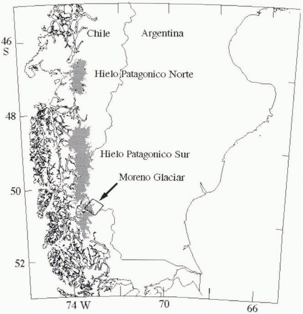
The Patagonia icefields are located at the southwestern tip of South America and consist of the northern icefield (Hielo Patagónico Norte) and the southern icefield (Hielo Patagónico Sur; HPS) (Fig. 1). Little glaciological information exists about these icefields, although they represent one of the largest ice masses in the world and the largest temperate ice mass in the Southern Hemisphere (Reference Warren and SugdenWarren and Sudgen, 1993).
Satellite imagery is naturally suited to the study of such regions. Landsat Thematic Mapper imagery has been used for large-scale inventory of the icefields (Reference Aniya, Sato, Naruse, Skvarca and CasassaAniya and others, 1996), but the range of applications of these data is limited. Only one cloud-free set of images of the entire icefield has been available since the inception of the Landsat satellite series.
Imaging radars are better adapted to conditions in these regions because they operate independent of cloud cover and solar illumination. In addition, when used interferometrically, imaging radars can yield precise information on the surface topography and ice velocity of entire icefields.
Radar coverage of the Patagonia icefields started in the 1990s with the Japanese JERS-1 radar, an L-band (24 cm wavelength) imaging radar system, which imaged various parts of the icefields in late 1993 and early 1994. The data quality was judged to be poor by Reference Aniya and NaruseAniya and Naruse (1995) clue to the lack of image contrast at the ice margin. The long time separation between repeat-pass JERS-1 acquisitions (24 days) also severely limits the possibility of interferometric analysis of the icefields. In March and October 1994, the NASA/Jet Propulsion Laboratory Shuttle Imaging Radar C (SIR-C) provided the first three-frequency, interferometric images of selected parts of the icefields (Reference Rignot, Forster and IsacksRignot and others, 1996a, b; Reference Rott, Stuefer, Siegel, Skvarca and EckstallerRott and others, 1998; unpublished information from R. R. Forster and others) and a nearly complete multi-channel coverage of HPS (Reference Forster, Isacks and DasForster and others, 1996). Finally in late 1995, the European Remote-sensing Satellite (ERS-1/2) provided comprehensive, interferometric coverage of the icefields.
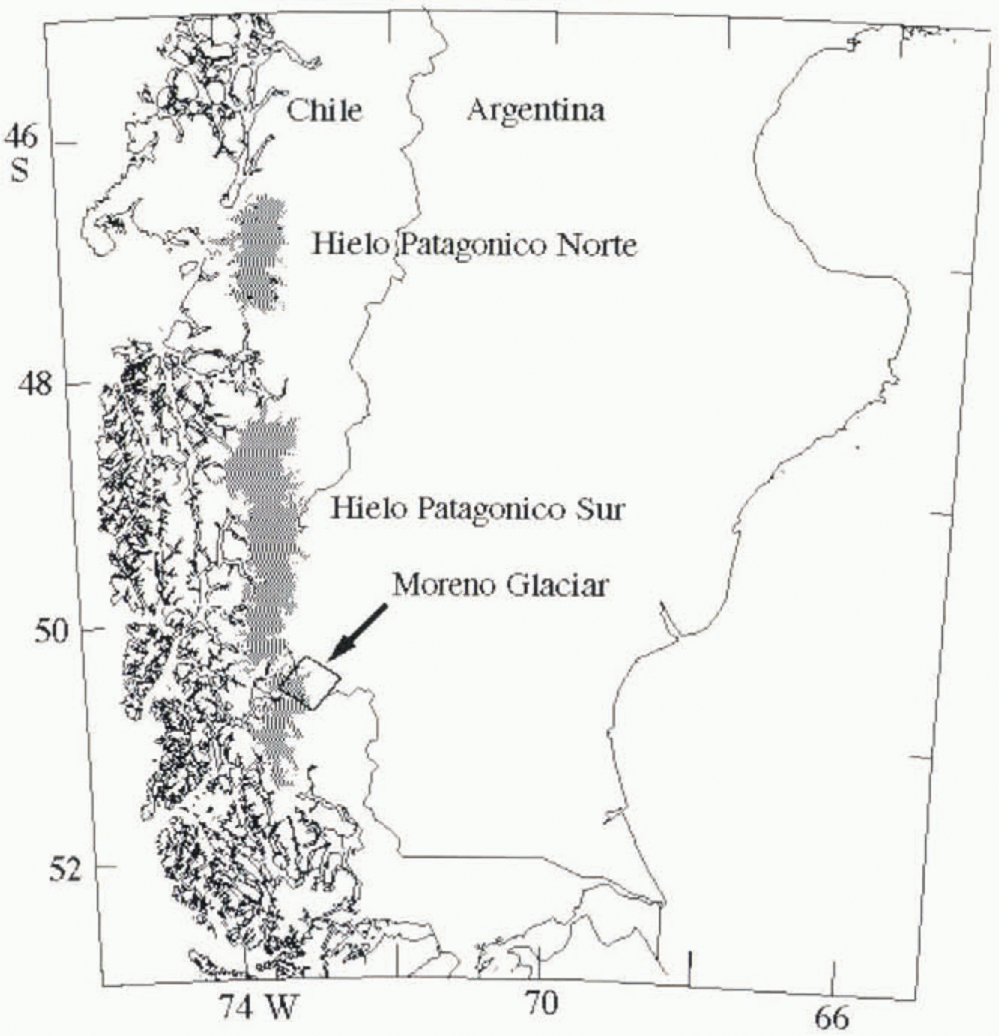
Fig. 1. Location map of Glacier Moreno, Argentina. Black box shows approximate location of SIR-C frame discussed in the paper. Shaded areas represent icefields.
Radar interferometry has its limitations. If the glacier surface changes too significantly between successive imaging acquisitions, for instance due to surface melting, the distribution of scatterers at the surface of the glacier is altered, the fading pattern of the radar signal is modified and the phase coherence of the radar signal is no longer preserved, making it impossible to measure glacier velocities interferometrically. Similarly, phase coherence is destroyed when the glacier deformation across an image pixel exceeds half the radar wavelength, for instance due to excessive strain rates along shear margins.
In areas of significant glacier weathering and/or deformation where radar interferometry is not always successful we propose a novel and complementary technique of data analysis for measuring ice velocity. The technique is known as “phase correlation method” in coherent optics (Reference Schaum and McHughSchaum and McHugh, 1991). It is related to the feature-tracking algorithm used with success on visible satellite imagery (Reference Bindschadler and ScambosBindschadler and Scambos, 1991) and more recently on repeat-pass ERS radar imagery (Fahnestock and others. 1993). There are, however, significant differences between the Landsat technique and the one presented here. The Landsat technique correlates the signal amplitude, whereas the phase correlation method correlates image speckle. Image speckle is a fundamental characteristic of the signal recorded by a coherent imaging system such as synthetic-aperture radar. Correlation of image speckle requires no recognizable image features at the glacier surface (e.g. crevasses), whereas correlation of the signal amplitude does. Correlation of image speckle can be effected at the sub-pixel level, whereas correlation of the signal amplitude is limited to one pixel. Finally, the phase correlation method is best used with image data acquired over short time periods (days to weeks), as in the case of radar interferometry, otherwise image speckle decorrelatcs. In contrast, the signal amplitude may remain correlated over long time periods, so the Landsat technique is best used with image data acquired over periods of months to years, meaning large glacier displacements compared to the pixel size.
An example application of the phase correlation method is presented here in the case of Glaciar Moreno, a major outlet glacier of HPS, which was imaged repeatedly for interferometric applications in October 1994 by SIR-C (Fig. 1). The dataset acquired by SIR-C over Glaciar Moreno is utilized to test the precision and limitation of the phase correlation method by comparing it with radar interferometry, and establish the level of synergy between the two techniques. The results are subsequently employed to infer first-order estimates of the ice-volume discharge and balance accumulation of Glaciar Moreno assuming stable ice-flow conditions.
Study Area
Glaciar Moreno, officially known as Glaciar Perito Moreno, occupies an area of 257 km2, 30 km long and 4 km wide in the terminal valley, with an accumulation area of 182 km2 (Reference Aniya and SkvarcaAniya and Skvarca, 1992). The glacier flows eastward from the eastern edge of HPS and calves into Lago Argentino where it divides the channel into the Canal de los Tempanos to the north and the Brazo Rico to the south. The glacier is well known for repeatedly damming up the Brazo Rico by reaching the opposite bank of the channel. Glaciar Moreno is one of the few Patagonian glaciers that is reached easily, and there is an abundance of historical and glaciological data on that glacier (Reference Aniya and SkvarcaAniya and Skvarca, 1992). Historical data on the position of the terminus suggest that the glacier has been more or less in steady state during the last century, in contrast to most other Patagonian glaciers which are currently experiencing a retreat (Reference Aniya, Sato, Naruse, Skvarca and CasassaAniya and others, 1997). This stability is supported by measurements of changes in surface elevation along a 3 km long area 5 km from the glacier front which revealed little change in ice thickness over a 2 year period (Reference Naruse and AniyaNaruse and Aniya, 1992). The glacier velocity, first measured 40 years ago by Reference Raffo, Colqui and MadejskiRaffo and others (1953) along a transverse profile 5–6 km from the glacier front, was re-measured at 11 locations in 1984 (Reference Naruse and AniyaNaruse and others, 1992).
Glaciar Moreno was imaged on 7, 9 and 10 October 1994 by NASA’s SIR-C on board the United Stales space shuttle. Endeavour, at both C– (λ = 5.67 cm) and L-band (24.23 cm) frequency, with vertical transmit-and-receive polarization, at an exact repeat-pass time interval of 23.618 hours (Fig. 2). Only the analysis of the L-band data is discussed here since the C-band data did not yield useful interferometric products due to the low phase coherence of the signal (see Rignot and others (1996a, b) for a discussion of the C-band and L-band data coherence). SIR-C illuminated the scene at an incidence angle of 34.37° away from vertical at the image center, an altitude of 218 km above ground, and a (center-range) distance of 271 km from the center of the scene. The image pixel spacing is 3.33 m in slant range (cross-track or line-of-sight direction), which is equivalent to 5.9 m in ground range (ground range = slant range/sin (34.37°)); and 5.21 m in the along-track or azimuth direction.

Fig. 2. Radar amplitude image of Glaciar Moreno acquired on 9 October 1994 by the SIR-C instrument at L-band frequency (24 cm wavelength), vertical transmit-and-receive polarization, at a mean incidence angle of 35°. The radar was flying from left to right, illuminating the ground from its left. While box delineates area of interest discussed in subsequent figures.
Methods
Interferometry
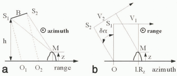
Repeat-pass radar interferometry measures surface deformation at the mm scale from the phase difference between radar signals collected on successive tracks over the same surface element (e.g. Reference Gabriel, Goldstein and ZebkerGabriel and others, 1989). The geometry of the interferometer is presented in Figure 3a. The interferometric phase for a point M on the ground is

where λ is the radar wavelength, S1M and S2M are the optical paths from M to the successive positions of the satellite S1 and S2, and S1S2 is the interferometric baseline, B. To produce an interferogram, the complex radar images (meaning amplitude and phase of the radar signal expressed as a complex number) are co-registered with sub-pixel precision, and a raw interferogram (here oversampled by a factor of 2) is formed by computing the cross-product of the registered complex images. The interferogram is then spatially averaged using a Hamming window (8 × 8 image pixels in size) and a compensation of the local phase slope which preserves the local fringe rate (Reference MichelMichel, 1997). Taking phase slope into account is crucial in areas of high shear strain (e.g. along the shear margins of a glacier) to preserve phase coherence during spatial averaging.

Fig. 3. Radar imaging geometry for (a) cross-track interferometry between positions S1 and S2 of the radar antenna illuminating a point M on the ground at elevation z from an altitude h, and where B is the interferometric baseline; and (b) along-track phase correlation method of a point M at elevation z. Velocity vectors, V1 and V2 of the two successive positions of the satellite form an angle δα in the vertical plane. Dotted circles in (a) and (b) denote an axis coming out of the plane of the figure toward the viewer. Rz is spatial resolution along track or azimuth.
The interferometric phase, δφ, is related to the orbital parameters (interferometric baseline, imaging angle, etc.), the surface topography and the surface deformation (Reference Zebker, Rosen, Goldstein, Gabriel and WernerZebker and others, 1994). The topography component of the signal may be removed using a prior-determined digital elevation model of the area or by combining two successive interferograms (Reference Gabriel, Goldstein and ZebkerGabriel and others, 1989). Here, the interferometric baseline was only a few tens of meters, so surface topography bad a negligible influence on the phase differences measured in a single interferogram (a full phase cycle (360°) corresponds to an 850 m change in elevation when the perpendicular baseline is 20 m).
An image of the temporal coherence of the phase, ρ, is obtained from the magnitude of the normalized cross-products. Phase coherence determines the statistical noise of the interferometric phase,

where N (here equal to 16) is the number of independent averaged samples used to generate the interferogram (Reference Rodriguez and MartinRodriguez and Martin, 1992). The uncertainly in glacier velocity measured along slant range is

Phase coherence varies spatially, as does σ v. With ρ = 0.4, a typical value for the SIR-C data, we have σ v = 0.8 cm d-1 in slant range, which is equivalent to 1.4 cm d-1 in ground range.
Phase correlation method
Surface velocity may also be derived from the correlation peak of image speckle. This second method is limited in precision by the pixel size (the precision of radar interferometry is limited by the size of the observing radar wavelength), but it provides two-dimensional vector displacements (cross-track displacements only for radar interferometry) and is intrinsically more robust to temporal decorrelation of the radar signal because it relies on the image intensity (phase information only for interferometry).
Along slant range, the range offsets are due to the glacier velocity along that direction, combined with a stereoscopic effect of the baseline which yields an elevation-dependent bias in range position. For a point M of the scene, the slant-range offset, δu, expressed in pixel units, is
where O1 and O2 are the ground-range positions corresponding to M in images 1 and 2, respectively (Fig. 3a), and R r is the pixel spacing in slant range.
For the same point M, the corresponding position S of the synthetic antenna at the time of imaging of M is the one which minimizes the distance MS. The velocity vectors, V1 and V2, of the successive orbits of the satellite are not necessarily colinear (Fig. 3b). The angle, δα, between the two vectors in the plane of incidence produces an elevation-dependent azimuth offset, δv, which, for a non-moving area, is expressed in pixel units as

where l is the line number with reference to the first line of the reference radar scene, R z is the azimuth or line spacing, z is the surface elevation and δv 0 is a constant offset. The first term on the righthand side of Equation (5) is elevation-dependent. The second term produces an azimuth ramp in the offset field.
To obtain reliable estimates of the glacier velocity, the image offsets, δu and δv, must be determined with sub-pixel precision. Sub-pixel-precision image registration is also required to form radar interferograms since the characteristic size of the fading pattern is of the order of 1–1.5 pixels. To compute the offsets with sub-pixel precision from the amplitude data, we use the phase correlation method of Reference Schaum and McHughSchaum and McHugh (1991). The deformation between the two images is approximated by a translation within Hanning windows 32 × 32 pixels in size. If a and b denote the amplitudes of two images translated by an amount δu in the range direction and δv is the azimuth direction, the Fourier transforms of a and b verify
where μ and v are the spatial frequencies along range and azimuth, respectively. We isolate the phase shift by computing

The inverse Fourier transform of C is a Dirac function, δ, located at a position (δu, δv)
The normalization of ab * in Equation (7) is a key feature of the phase correlation method which is responsible for the narrow shape of the correlation peak and an enhancement of its signal-to-noise ratio (SNR).
The numerical Fourier transform of the images leads to the determination of the correlation peak in pixel units. The SNR of the correlation peak is not optimum because of the non-overlapping areas of a and b, non-linear deformations associated with topography and velocity gradients within the sliding window, and changes in fading pattern (which are responsible for phase decorrelation). To reduce the effect of non-overlapping areas, we first evaluate the integer shift between the two images using the peak value of C, extract two new sub-images 16 × 16 pixels in size so that the non-overlapping areas do not exceed one pixel in size, and search again for the position of the correlation peak. A sub-pixel position of the correlation peak is then estimated as the barycenter (or weighted average) of the peak using

where V is a 3 × 3 neighborhood of the correlation peak, and k and l are the column and line indexes, respectively.
The conservation of the total energy of C,

allows for a practical evaluation of the SNR of the correlation peak in both range (u) and azimuth (v),

The uncertainty in δv and δv is a function ?f S u and S v , respectively.
To test the relationship between SNR and offset precision, we employed two computer-generated images, 1000 × 1000 pixels in size, with a known offset field (linearly varying offsets), calculated the offsets and SNRs as described above, and obtained the results shown in Figure 4. As expected, low SNR values yield high offset errors. To obtain an offset precision of one-30th of the pixel size, the SNR of the correlation peak needs to be better than 0.15.
The advantage of computing both S u and S v rather than only one “global” SNR is that it limits the possibility of false matches associated with oblong correlation peaks, meaning a correlation peak which is narrow in one direction but broad in another, as recorded, for instance, in the presence of a train of crevasses. Here, a false match may be detected when either S u or S v is below a threshold (typically 0.15). The vector SNR measurements thereby procure more control on the quality of the vector offsets.

Fig. 4. Precisian of image offsets expressed in pixel spacing as a function of the SNR of the image, correlation peak expressed in linear unit in the case of computer-generated test data.
Results
Velocity Estimates
The baseline and topography effects were removed automatically from both the SIR-C interferograms and the SIR-C offset map using an average fringe rate. This simplification is justified by the short interferometric baseline of the data and the low glacier slope of Glaciar Moreno.
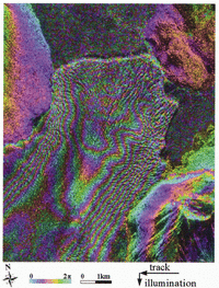
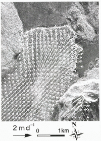
The L-band interferogram shown in Figure 5 was unwrapped (meaning the fringes were counted from a zero reference to restitute absolute phase values) using Goldstein and others’ (1988) unwrapping technique, to yield the result shown in Figure 6. Unwrapping could not be performed successfully near the glacier front and at high elevation because of low phase coherence in these regions. The phase correlation method conversely performed well over the entire glacier to provide two-dimensional velocities, displayed on a regular grid in Figure 7.
Equations (1) and (4) show that the unwrapped phase, δφ, and the range offset, δu, are linearly related via

Figure 8a and b show comparisons between the interferometric velocities and the slant-range image offsets measured along the transverse and longitudinal profiles shown in Figure 6. Systematic errors introduced by topographic features and baseline errors have the same effect on both methods, so the difference between the two curves represents an unbiased comparison of the two techniques.
The average uncertainty in interferometric velocity is 1 cm d-1 based on the statistical noise of the interferometric phase (the error bar is too small to be visible in Figure 8a and b), which translates into 1.8 cm d-1 of uncertainty in ground-range motion. The average difference between the offset velocity and the interferometry velocity is 8 cm d-1 in slant range, or 14 cm d-1 in ground range (50 m a-1), which is equivalent to a precision of detection of the offsets of one-30th of a pixel. In profile 2, the calculated offset error is larger along the glacier margins (up to 10–15 cm d-1) because the SNR is lower. In general, the offsets remain within one calculated standard deviation of the interferometry measurements. One exception is found along the northern margin of profile 2 where the offset precision is apparently overestimated.

Fig. 5. Radar interferogram of Glaciar Moreno, obtained by combining data acquired on 9 and 10 October 1994 by the SIR-C instrument at L-band frequency. Each fringe, or 360° variation in phase, going from blue to purple, yellow and blue again, represents a 12 cm displacement of the glacier surface in the line of sight of the radar.
More precise ice velocities may be obtained from the phase correlation method using data acquired with a longer time separation. The signal correlation may eventually decrease after a few days, so there is an optimal time period for our technique to be used. More accurate velocity measurements may also be obtained by using larger-size averaging windows when computing the image correlation peak, at the expense of spatial resolution.
Phase unwrapping fails when phase coherence drops below about 0.2, in which case ice velocity cannot be measured interferometrically. The phase correlation method becomes unreliable when the correlation peak SNR drops below 0.06, which corresponds to an offset error of 0.5 pixels (Fig. 4). Phase coherence and correlation peak SNR are independent variables, so the performance of the phase correlation method cannot be predicted in regions where phase coherence is low. The phase correlation method, however, typically works best where radar interferometry breaks down, for instance in areas experiencing significant weathering (ablation or precipitation) and/or large glacier deformation.

Fig. 6. Unwrapped radar interferogram (shown in Fig. 5) of Glaciar Moreno, and location of profiles 1 and 2 used for the comparison between interferometry and the phase correlation method, and of the 300 m elevation contour line used to estimate ice discharge.
Comparison with Prior Measurements
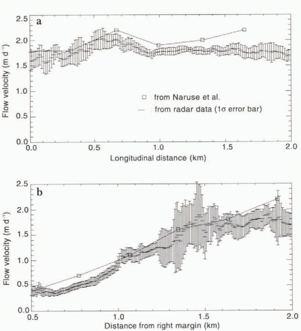
Using an electronic distance meter, Reference Naruse and AniyaNaruse and others (1992) measured the glacier velocity at 11 points and derived vertical strain rates. Half of the measurements were collected along a transverse profile located 4 km from the ice front, running from the right margin of the glacier to its middle section. The other measurements were collected along a longitudinal profile about 2 km from the right margin, and 4 km from the ice front. Figure 9 compares their results with the SIR-C measurements. The comparison shows no significant change in ice velocity between November 1990 and October 1994, except perhaps near the ice from where Naruse and others’ (1992) velocity measurements are expected to be least precise due to the chaotic nature of the glacier surface.
Surface Strain Rates
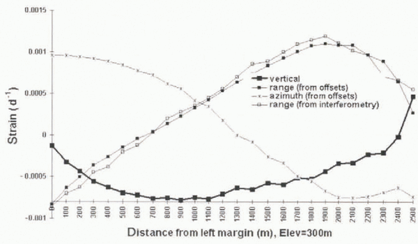
The slant-range strain rate, ![]() , and the azimuth strain rate,
, and the azimuth strain rate, ![]() , were calculated by differentiating the two-dimensional offset map using a Lagrangian operator. The strain rates were averaged using a 5 × 5 pixel window (meaning 240 m × 240 m in size on the ground) to enhance the SNR. The values obtained along the 300 m elevation contour line are shown in Figure 10 after interpolation to a 100 m spacing. The measurement uncertainty, estimated for each method by calculating the standard deviation in strain rate within 5 × 5 windows, is 10-5 d-1 for the interferometry data, and 10-4 d-1 for the offsets.
, were calculated by differentiating the two-dimensional offset map using a Lagrangian operator. The strain rates were averaged using a 5 × 5 pixel window (meaning 240 m × 240 m in size on the ground) to enhance the SNR. The values obtained along the 300 m elevation contour line are shown in Figure 10 after interpolation to a 100 m spacing. The measurement uncertainty, estimated for each method by calculating the standard deviation in strain rate within 5 × 5 windows, is 10-5 d-1 for the interferometry data, and 10-4 d-1 for the offsets.

Fig. 7. Ice-velocity vector of Glaciar Moreno within the area delineated with a while box in Figure 2 and derived from the phase correlation method. Flow vectors are overlaid on the radar brightness of the scene at L-band frequency. Spacing between flow vectors is 320 m.
The vertical strain rate, ![]() is deduced from the horizontal strain rates assuming incompressibility of the ice:
is deduced from the horizontal strain rates assuming incompressibility of the ice:

where i is the incidence angle of the radar illumination from vertical.
Ice Discharge
While most Patagonian glaciers seem to be retreating (Reference Aniya, Sato, Naruse, Skvarca and CasassaAniya and others, 1997), Glaciar Moreno seems to be stable. To obtain first-order estimates of the ice volume discharge and balance accumulation of Glaciar Moreno, we use a model to infer the glacier thickness from the measured vertical strain rates combined with prior data on surface net balance.
The equation of steady-state mass balance (Paterson, 1994) dictates

where Ḃ is the glacier net balance (sum of accumulation minus ablation, and Ḃ < 0 for net ablation), H is the glacier thickness, and V x is the glacier velocity along an x axis which follows a flowline and points down-glacier. Reference Aniya and NaruseNaruse and others (1995) estimated Ḃ to be 11.2 m a-1 w.e. at 350 m elevation, or 12.2 m ice a-1, and that Ḃ varies with surface elevation with a gradient of 0.015 a-1. The glacier net balance at 300 m elevation is therefore estimated to be 13 m a-1 ice volume, or 3.56 cm ice d-1.

Fig. 8. Comparison of velocities measured in slant range with the phase correlation method and radar-interferometry estimates along (a) longitudinal profile 1 in Figure 6, and (b) transverse profile 2 in Figure 6. Error bars correspond to one standard deviation in ice velocity. Interferometric measurements plotted on the horizontal axis (zero velocity) correspond to data points for which phase unwrapping was not successful and hence ice velocity could not be estimated interferometrically. Positions are measured in reference to south bank of glacier for profile 1, and glacier terminus for profile 2.

Fig. 9. Comparison between velocities measured by Reference Naruse and AniyaNaruse and others (1992) and those measured using the phase correlation method on the SIR-C data along (a) a longitudinal profile, and (b) a transverse profile. (See text for location of profiles.) Error bars from Naruse and others’ (1992) data are not available.

Fig. 10. Strain rate (per day) of Glaciar Moreno along the 300 m elevation contour profile in Figure 6, along the range direction (both interferometry and phase correlation method (called offsets)), azimuth (offsets only) and vertical (offsets only). Each value is calculated using a 240 m spacing, and the results are interpolated every 100 m.
The gradient in glacier thickness in the longitudinal direction, ?H/?X, not known from prior field experiments, is assumed to be constant across the glacier width. To estimate its value, we find the (two) positions along the profile for which ![]() equals zero:
equals zero:

The resulting thickness profile is shown in Figure 11. The precision is 30%, or 200 m, based on the uncertainty in strain-rate, velocity and ablation data. The error in ice thickness could be larger if our assumption about the gradient in ice thickness is unrealistic.
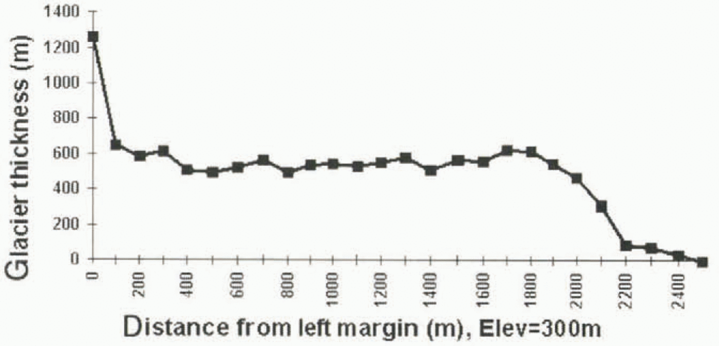
Fig. 11. Ice thickness of Glaciar Moreno at 300 m elevation deduced from mass conservation assuming steady flow conditions and using the vertical strain rates measured with SIR-C combined with prior data on mass ablation (Reference Aniya and NaruseNaruse and others, 1995). The precision in ice thickness is 200 m, worsening along the side margins due to a lower SNR. The first point of the profile (distance = 0) is a singular point in the inversion which produces an erroneous estimation of ice thickness.Ice thickness of Glaciar Moreno at 300 m elevation deduced from mass conservation assuming steady flow conditions and using the vertical strain rates measured with SIR-C combined with prior data on mass ablation (Reference Aniya and NaruseNaruse and others, 1995). The precision in ice thickness is 200 m, worsening along the side margins due to a lower SNR. The first point of the profile (distance = 0) is a singular point in the inversion which produces an erroneous estimation of ice thickness.Ice thickness of Glaciar Moreno at 300 m elevation deduced from mass conservation assuming steady flow conditions and using the vertical strain rates measured with SIR-C combined with prior data on mass ablation (Reference Aniya and NaruseNaruse and others, 1995). The precision in ice thickness is 200 m, worsening along the side margins due to a lower SNR. The first point of the profile (distance = 0) is a singular point in the inversion which produces an erroneous estimation of ice thickness.Ice thickness of Glaciar Moreno at 300 m elevation deduced from mass conservation assuming steady flow conditions and using the vertical strain rates measured with SIR-C combined with prior data on mass ablation (Reference Aniya and NaruseNaruse and others, 1995). The precision in ice thickness is 200 m, worsening along the side margins due to a lower SNR. The first point of the profile (distance = 0) is a singular point in the inversion which produces an erroneous estimation of ice thickness.
The ice volume flux, Φ, is deduced using

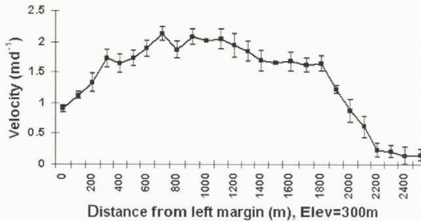
along the 300 m contour, where n is the normal to the contour and V is the ice-velocity vector (Fig 12). We assume that the velocity vector does nut change with depth, meaning that the glacier sliding velocity is equal to its surface velocity. The result is an ice flux of 0.6 ± 0.2 km3 ice a-1 at 300 m elevation. From the gradient in melt rate measured by Reference Aniya and NaruseNaruse and others (1995) and the published glacier topographic map, we calculate the glacier net balance between the 300 m profile and the equilibrium line (1150 m). The calculated net balance is added to our estimated ice flux to deduce an ice flux at the equilibrium line of 1.1 ± 0.2 km3 ice a-1. Averaged over the entire accumulation area (182 km2), the glacier discharge corresponds to a balance accumulation of 6 ± 1 m ice a-1.

Fig. 12. Ice velocity of Glaciar Moreno in the direction perpendicular to the 300 m elevation contour profile shown in Figure 6 and derived from the phase correlation method. Error bars correspond to one standard deviation in ice velocity.
An ice core drilled at 2680 m elevation, near the top of the accumulation area of Glaciar Moreno (Reference Aristarain and DelmasAristarain and Delmas, 1993), yielded an accumulation rate of 1.2 m a-1 w.e., deemed too low by Reference Aniya and NaruseNaruse and others (1995). Using precipitation maps published in Chile, Reference Aniya and NaruseNaruse and others (1995) suggested instead that snow accumulation reaches 8 m a-1 at 2000 m elevation, linearly decreasing with elevation. They quote a mean precipitation over the eastern ice-covered areas of 6.4 m a-1. Our result, which represents a balance accumulation over the accumulation area of a stable glacier, is consistent with their interpretation and close to their estimate of mean precipitation along the eastern flank of HPS.
More recently, Reference Rott, Stuefer, Siegel, Skvarca and EckstallerRott and others (1998) conducted field surveys on Glaciar Moreno which produced a complete ice-thickness seismic profile a few km above the 300 m elevation contour. The measured ice thickness averaged 440 m, compared to 490 m in our inversion. The measured thickness profile has, however, a more pronounced parabolic shape than that shown in Figure 12. From their measurements, Rott and others (l998) deduced an annual net accumulation of 5.54 ± 0.5 m water a-1 from their data, which is within the error bounds of our estimate.
Conclusions
The study demonstrates the possibility of obtaining accurate ice velocities and strain rates from the phase correlation method using satellite radar images acquired with a short repeat-pass time interval compatible with that required for radar interferometry applications. The phase correlation method provides two-dimensional vector velocities, over a large range of glacier conditions and changes in glacier scattering. Current imaging radar systems available for interferometric applications over glaciated terrain, such as ERS and JERS, do not oiler repeal-pass cycles that are short enough for measuring ice velocities of fast-moving outlet glaciers in Patagonia or Alaska or along the western and eastern coasts of Greenland. The phase correlation method is an indispensable complementary tool of analysis for data collected by these instruments.
In the case of the ERS system, the pixel spacing is 20 m on the ground in the across-track direction (7.9 m along the line of sight), and 4 m in azimuth. Extrapolation of the SIR-C results to the case of ERS suggests that the phase correlation method will measure ice velocity with a precision of 13 cm d-1 (49 m a-1) in the along-track direction, and 67 cm d-1 (240 m a-1) in the cross-track (range) direction. This level of precision is sufficient to provide first-order estimates of the ice velocity of fast-moving ice fronts.
Acknowledgements
This work was partially performed at the Jet Propulsion Laboratory, California Institute of Technology, under a contract with the National Aeronautics and Space Administration. We thank J. Taboury of the Institut d’Optique Théorique et Appliquée, Orsay, France, and J. P. Avouac of the Laboratoire de Détection et de Géophysique, Bruyèresle-Châtel, France, for useful discussions during this project.