


1. INTRODUCTION AND AIMS
Many supraglacial lakes (hereafter ‘lakes’) that form annually within the ablation zone of the Greenland ice sheet (GrIS) drain in the mid- to late season, while others simply freeze in the autumn (Selmes and others, Reference Selmes, Murray and James2013; Tedesco and others, Reference Tedesco2013; Miles and others, Reference Miles, Willis, Benedek, Williamson and Tedesco2017). Draining lakes can be classified as either ‘rapidly’ or ‘slowly’ draining (Chu, Reference Chu2014; Nienow and others, Reference Nienow, Sole, Slater and Cowton2017). Rapid events occur in situ over hours to several days by a hydraulically-driven fracture mechanism (‘hydrofracture’) (e.g. Das and others, Reference Das2008; Doyle and others, Reference Doyle2013; Tedesco and others, Reference Tedesco2013; Stevens and others, Reference Stevens2015), with ~10% of lakes thought to drain in this way across the whole GrIS (Selmes and others, Reference Selmes, Murray and James2011, Reference Selmes, Murray and James2013). Slow events occur over days to weeks when a lake overflows and incises a surface outlet stream (Hoffman and others, Reference Hoffman, Catania, Neumann, Andrews and Rumrill2011; Tedesco and others, Reference Tedesco2013). Although the two processes are distinct, they can influence each other if, for example, a stream from a slowly draining lake is tapped by a moulin, directing surface water to the ice-sheet bed, and causing uplift or basal sliding that may then induce hydrofracture and rapid drainage nearby (Tedesco and others, Reference Tedesco2013; Stevens and others, Reference Stevens2015).
All lakes affect the GrIS's mass balance because they have a lower albedo than the surrounding bare ice, enhancing surface ablation (Lüthje and others, Reference Lüthje, Pedersen, Reeh and Greuell2006; Tedesco and Steiner, Reference Tedesco2011; Tedesco and others, Reference Tedesco and Steiner2012). However, draining lakes, and particularly those draining rapidly, are of additional interest because they affect ice velocities via the delivery of large meltwater volumes to the ice-sheet bed (e.g. Zwally and others, Reference Zwally2002; van de Wal and others, Reference van de Wal2008; Schoof, Reference Schoof2010; Colgan and others, Reference Colgan2011a; Cowton and others, Reference Cowton2013; Fitzpatrick and others, Reference Fitzpatrick2013; Bougamont and others, Reference Bougamont2014 Dow and others, Reference Dow, Kulessa, Rutt, Doyle and Hubbard2014). These meltwater pulses can overwhelm the capacity of the subglacial drainage system, lower subglacial effective pressure, enhance basal sliding and increase surface ice velocity by >200% of background winter levels over short (hourly–daily) timescales (Shepherd and others, Reference Shepherd2009; Schoof, Reference Schoof2010; Hoffman and others, Reference Hoffman, Catania, Neumann, Andrews and Rumrill2011; Bartholomew and others, Reference Bartholomew2011a,Reference Bartholomewb, Reference Bartholomew2012; Banwell and others, Reference Banwell2013; Tedesco and others, Reference Tedesco2013; Andrews and others, Reference Andrews2014; Bougamont and others, Reference Bougamont2014; Kulessa and others, Reference Kulessa2017). Hydrofracture events also open up moulins that can consequently transport surface meltwater to the bed, potentially promoting sliding over longer (weekly–seasonal) timescales (Zwally and others, Reference Zwally2002; Joughin and others, Reference Joughin2008, Reference Joughin2013; Bartholomew and others, Reference Bartholomew2010; Colgan and others, Reference Colgan2011b; Palmer and others, Reference Palmer, Shepherd, Nienow and Joughin2011; Banwell and others, Reference Banwell2013, Reference Banwell, Arnold, Willis, Tedesco and Ahlstrøm2016; Cowton and others, Reference Cowton2013; Sole and others, Reference Sole2013; Tedstone and others, Reference Tedstone, Nienow, Gourmelen and Sole2014; Koziol and others, Reference Koziol, Arnold, Pope and Colgan2017). This moulin opening is particularly important because cold-based ice at central depths of the GrIS acts as a thermal barrier to water penetration, likely meaning that water can reach the ice bed only through such fractures (Irvine-Fynn and others, Reference Irvine-Fynn, Hodson, Moorman, Vatne and Hubbard2011; Lüthi and others, Reference Lüthi2015; Greenwood and others, Reference Greenwood, Clason, Helanow and Margold2016; Poinar and others, Reference Poinar, Joughin, Lenaerts and van den Broeke2017).
There is debate, however, over the significance of such drainage-driven speed-up over longer (seasonal–decadal) timescales, since the subsequent evolution of subglacial conduits to hydraulically efficient conditions may increase subglacial effective pressures sufficiently to reduce ice velocities, thus offsetting the impact of the earlier speed-ups (Palmer and others, Reference Palmer, Shepherd, Nienow and Joughin2011; Sundal and others, Reference Sundal2011; Bartholomew and others, Reference Bartholomew2011a; Banwell and others, Reference Banwell2013, Reference Banwell, Arnold, Willis, Tedesco and Ahlstrøm2016; Chandler and others, Reference Chandler2013; Andrews and others, Reference Andrews2014; Mayaud and others, Reference Mayaud, Banwell, Arnold and Willis2014; Tedstone and others, Reference Tedstone, Nienow, Gourmelen and Sole2014, Reference Tedstone2015). Finally, rapid lake drainage can affect ice dynamics through the input of relatively warm surface water to the colder ice beneath, promoting faster ice flow due to the strong dependency of ice-deformation rates on ice temperature (Phillips and others, Reference Phillips, Rajaram and Steffen2010, Reference Phillips, Rajaram, Colgan, Steffen and Abdalati2013), although the significance of this process is debated (Poinar and others, Reference Poinar, Joughin, Lenaerts and van den Broeke2017).
To date, most of the above phenomena have been studied for ice-marginal regions of the GrIS, typically below ~1600 m ice-surface elevation. However, recent research has started to examine whether similar processes might extend to the interior regions of the GrIS in the future as surface melt rates increase and lakes form at higher elevations (Liang and others, Reference Liang2012; Howat and others, Reference Howat, de la Peña, van Angelen, Lenaerts and van den Broeke2013; Doyle and others, Reference Doyle2014; Fitzpatrick and others, Reference Fitzpatrick2014; Leeson and others, Reference Leeson2015; Poinar and others, Reference Poinar2015; Gledhill and Williamson, Reference Gledhill and Williamson2018). Whether or not there is an altitudinal limit to rapid lake drainage, due to the thicker ice and limited crevassing that may impede hydrofracture, is currently unknown (Poinar and others, Reference Poinar2015). If hydrofracture can occur at these elevations, it seems probable that rapid lake drainage and the subsequent input of meltwater via moulins will cause sustained ice speed-ups over seasonal to annual timescales. This would be likely due to enhanced ice deformation via ice-sheet warming (Phillips and others, Reference Phillips, Rajaram and Steffen2010, Reference Phillips, Rajaram, Colgan, Steffen and Abdalati2013), and enhanced basal sliding due to the thick ice (promoting high creep-closure rates) and low ice-surface slopes (producing low subglacial hydraulic-potential gradients) restricting the evolution of subglacial drainage from distributed to channelised (Meierbachtol and others, Reference Meierbachtol, Harper and Humphrey2013; Dow and others, Reference Dow, Kulessa, Rutt, Doyle and Hubbard2014; Doyle and others, Reference Doyle2014; Poinar and others, Reference Poinar2015).
It is essential, therefore, to understand the present distribution of rapid lake-drainage events and the factors that may control the hydrofracture process across the GrIS. If this were better understood, the location, timing and magnitude of rapid lake-drainage events could be incorporated with an improved physical basis into coupled hydrology-ice flow models of the GrIS, which could then be used to predict future ice-sheet dynamics with greater certainty. So far, research into rapid lake drainage has involved fieldwork (Das and others, Reference Das2008; Doyle and others, Reference Doyle2013; Tedesco and others, Reference Tedesco2013; Stevens and others, Reference Stevens2015), numerical modelling (Banwell and others, Reference Banwell, Willis and Arnold2012, Reference Banwell2013, Reference Banwell, Arnold, Willis, Tedesco and Ahlstrøm2016; Clason and others, Reference Clason2012, Reference Clason, Mair, Burgess and Nienow2015; Arnold and others, Reference Arnold, Banwell and Willis2014; Koziol and others, Reference Koziol, Arnold, Pope and Colgan2017) or satellite remote sensing (Box and Ski, Reference Box and Ski2007; Sundal and others, Reference Sundal2009; Selmes and others, Reference Selmes, Murray and James2011, Reference Selmes, Murray and James2013; Liang and others, Reference Liang2012; Johansson and others, Reference Johansson, Jansson and Brown2013; Morriss and others, Reference Morriss2013; Fitzpatrick and others, Reference Fitzpatrick2014; Everett and others, Reference Everett2016; Chen and others, Reference Chen, Howat and de la Peña2017; Cooley and Christoffersen, Reference Cooley and Christoffersen2017; Miles and others, Reference Miles, Willis, Benedek, Williamson and Tedesco2017; Williamson and others, Reference Williamson, Arnold, Banwell and Willis2017).
Collectively, this research has produced a consensus on the general controls on rapid lake drainage for different regions of the GrIS: rapid drainage typically occurs at progressively higher elevations over the melt season, with the usually smaller ice-marginal lakes draining before the larger ones further inland. Currently, several factors thought to control hydrofracture are used to explain rapid lake drainage since it is generally acknowledged that for a fracture to propagate from the ice-sheet surface to the bed, it must remain water-filled for its entire depth (Alley and others, Reference Alley, Dupont, Parizek and Anandakrishnan2005; van der Veen, Reference van der Veen2007; Tsai and Rice, Reference Tsai and Rice2010). This suggests that a critical water-volume threshold may be needed to initiate rapid lake drainage, with the value of this threshold necessarily being higher for thicker ice. Modelling studies therefore link water volume and local ice thickness to calculate ‘fracture area’ thresholds for rapid lake drainage, where rapid drainage is triggered once a lake's water volume exceeds the local ice thickness multiplied by a prescribed map-plane fracture area (Clason and others, Reference Clason2012, Reference Clason, Mair, Burgess and Nienow2015; Banwell and others, Reference Banwell2013, Reference Banwell, Arnold, Willis, Tedesco and Ahlstrøm2016; Arnold and others, Reference Arnold, Banwell and Willis2014; Koziol and others, Reference Koziol, Arnold, Pope and Colgan2017). The underlying physical basis to the fracture area threshold is that the quantity of surface meltwater controls a fracture's filling and expansion, as well as ensuring that it remains open by offsetting refreezing (van der Veen, Reference van der Veen2007; Krawczynski and others, Reference Krawczynski, Behn, Das and Joughin2009). However, these models typically display an equally high performance for a variety of water-volume thresholds (Table 1). It is possible, therefore, that water volume may be important in controlling hydrofracture but only if one or more additional controls work alongside it. For example, field data from Stevens and others (Reference Stevens2015) suggest that a local stress perturbation (caused by the delivery of meltwater to the ice-sheet bed via a nearby moulin) is required to initiate hydrofracture, with a certain lake area or volume being only a prerequisite for, rather than the driver of, drainage. However, this study was limited to a single lake (meaning it is unclear whether similar processes operate elsewhere) and it did not examine the potential influence of other controls apart from this, such as those we identify later (Table 2). Moreover, theoretical, field-based, remote sensing and modelling studies have shown that rapidly draining lakes, as well as containing a wide variety of water volumes prior to drainage, have seemingly no common characteristics among the factors that might be influential in causing rapid drainage (Table 1).
Table 1. Hydrological, glaciological and other notable characteristics of rapidly draining lakes on the GrIS identified in previous studies

* Theoretical work was insensitive to assumed tension value.
† Calculated by multiplying the study's lower lake-water-depth bound (2 m) by the lower lake-area bound (a 0.25 km-diameter lake approximated as a perfect circle).
‡ Study on John Evans glacier, Ellesmere Island, Canada, rather than the GrIS, but also for cold-based ice (at ~ −10 °C).
§ Study assumes value based on summer 2011 measurements.
|| Study identifies only ‘outburst’ events, but does not determine the mechanism of ‘outburst’ (either lake overtopping or hydrofracture).
¶ Smallest value listed in the study, which only presented the 50 largest events.
** Lower bound, limited to the smallest lake size (55 × 30 m pixels = 0.0495 km2) tracked in the study.
†† Value calculated by multiplying the study's fracture area threshold by an ice thickness of 1 km.
‡‡ Value producing best match between modelled and observed proglacial discharge.
§§ Value producing best match between modelled and satellite-observed (Landsat 7 ETM+) volumes, but volumes were likely overestimated (Pope and others, Reference Pope2016).
|||| Model sensitivity tested within this range to show how lakes were partitioned into different drainage types based on adjusting this value.
Table 2. Potential controlling factors on hydrofracture investigated in this study. Hydrological and morphological data are at the individual lake scale (i.e. kilometres to several kilometres), glaciological data are at the scale of the ice underlying or adjacent to lakes (i.e. kilometres to tens of kilometres), while surface-mass-balance (SMB) data cover synoptic-scale meteorological processes that typically operate across the entire regions (i.e. tens of kilometres)

* Average ice flow derived from x and y components of MEaSUREs winter velocity data.
† Derived from ice-surface elevation data, which were first coarsened to 1 km resolution to ensure slopes were derived across rather than within lake basins, then interpolated (using a nearest-neighbour technique) to 250 m resolution for consistency with the other data.
‡ Lake basin is defined as the lake area at the lake's maximum extent (for non-rapidly draining lakes) or on the day prior to hydrofracture (for rapidly draining lakes).
§ Catchment refers to a lake's ice-surface catchment, determined with MATLAB's ‘watershed’ function (using a default eight-connected neighbourhood).
Taken together, existing work shows no agreement on the precise hydrological or glaciological controls on rapid lake drainage (notably the required lake area, volume or depth, or the ice-stress regime), with the possibility that the controls vary between lakes and between or within different sectors of the GrIS (for example, between land- and marine-terminating outlets, or interior and ice-marginal regions). There is a need, therefore, to investigate whether the observations from individual lakes apply more widely, whether additional controls are important in driving lake drainage, and whether the controls are spatiotemporally uniform or variable between sectors of the GrIS and times of the year. Towards this end, Selmes (unpublished 2011 Swansea University Ph.D. thesis) examined how ice-sheet thickness, ice-surface slope and ice-surface velocity may influence rapid lake drainage identified from MODIS imagery over the entire GrIS in 2005–09, but found statistically insignificant relationships for all the controls investigated. The study may have been compromised, however, because: (i) the data were of coarse (~5 km) resolution; (ii) the study was over the entire GrIS rather than for specific regions, making patterns difficult to recognise; (iii) the statistical relationships were computed with respect only to lake areas and not lake volumes, and; (iv) the analysis was restricted to linear correlation.
To address the limited previous work, our objective here is to examine the hydrological and glaciological controls on rapid lake drainage suggested by previous research, as well as to examine a variety of other factors that may also control the location, timing and magnitude of rapid lake drainage. This objective is addressed using rigorous, regional-scale statistical Exploratory Data Analysis (EDA), which is an approach to explore existing hypotheses, to re-evaluate them with new data and perhaps to propose new hypotheses or to suggest future research directions (Tukey, Reference Tukey1977). The EDA focuses on two locations: the land-terminating Paakitsoq and the marine-terminating Store Glacier regions of West Greenland (Fig. 1), for the 2014 melt season. We conduct this analysis for a large sample of 213 lakes to determine whether the insights gained from previous field studies (e.g. Doyle and others, Reference Doyle2013; Tedesco and others, Reference Tedesco2013; Stevens and others, Reference Stevens2015) for individual lakes more widely apply. The EDA aims to:
1. Identify the distribution of rapidly and non-rapidly draining lake types within the two regions, including their areas, volumes and their drainage dates or the dates when they reach their maximum extent.

Fig. 1. The (a) Paakitsoq and (b) Store Glacier regions of West Greenland (inset). Note the difference in horizontal scale between the two panels. Polygons indicate whether lakes observed in 2014 MODIS imagery drain rapidly (triangles; ⩽4 days) or not (circles; >4 days), colour-coded according to area immediately prior to drainage for rapidly draining lakes and area when reaching their maximum seasonal extents for non-rapidly draining lakes (see Section 3.1). The GrIS margin (thick black line) and ice-surface elevation contours (thin black lines) from Howat and others (Reference Howat, Negrete and Smith2014) are shown.
2. Derive data for a variety of potential controlling factors that may explain the observed distributions of the lake types within the regions.
3. Analyse whether there are statistically significant differences between the two lake types in terms of the potential controlling factors.
4. Analyse whether statistically significant correlations exist between the potential controlling factors and both lake areas or volumes for the two lake types.

Collectively, the above analysis might indicate links between one or multiple factors and the incidence of hydrofracture on the GrIS.
2. METHODS, DATA AND STUDY SITES
Here, we describe: (i) the methods used to identify rapidly and non-rapidly draining lakes (Section 2.1); (ii) the original datasets used in the EDA, and the derivation of various factors from these data that may control the spatiotemporal patterns of rapid lake drainage, including the justification for including them (Section 2.2); (iii) the statistical techniques for the EDA (Section 2.3); and, (iv) the rationale for choosing the study sites (Section 2.4).
2.1. Identifying rapidly and non-rapidly draining lakes
For the first aim of the study, involving detecting rapid lake-drainage events and thus the distribution of rapidly draining and non-rapidly draining lakes, we used the Fully Automated Supraglacial lake Tracking (FAST) algorithm (Williamson and others, Reference Williamson, Arnold, Banwell and Willis2017). Images derived from the MODIS MOD09 surface-reflectance product from 1 May to 30 September 2014 were chosen, totalling 153 images. Bands 1 (red; 0.620–0.670 μm) and 6 (1.628–1.652 µm) were required; band-1 data are distributed at native ~250 m resolution, while band-6 data have ~500 m resolution. We chose MODIS imagery to exploit the daily temporal resolution of the record, crucial for identifying rapid lake drainage since hydrofracture occurs in hours to days, although we recognised there was a trade-off with MODIS's lower spatial resolution (Leeson and others, Reference Leeson2013; Miles and others, Reference Miles, Willis, Benedek, Williamson and Tedesco2017; Williamson and others, Reference Williamson, Arnold, Banwell and Willis2017).
Williamson and others (Reference Williamson, Arnold, Banwell and Willis2017) provide full details of the FAST algorithm, but, briefly, it incorporates the following steps:
1. MODIS images are pre-processed using the MODIS Reprojection Tool Swath (version 2.2), including reprojection to the Polar Stereographic grid (EPSG: 3413) using bilinear interpolation, and sharpening of band-6 data from 500 m resolution to match band 1's 250 m resolution.
2. MODIS tiles are cropped automatically to the study regions using a georeferenced mask, ice-marginal areas are removed using the Greenland Ice Mapping Project ice-sheet mask (Howat and others, Reference Howat, Negrete and Smith2014), and clouds and cloud shadows are filtered when band-6 values exceed 0.15.
3. Lake areas are derived for each image using dynamic thresholding of the red band. This approach identifies a water-covered pixel when the reflectance of the central pixel in a 25 × 25-pixel moving window is below 0.640 of the mean red-band reflectance within the whole window. MODIS lake areas derived by this method have a RMSE of 0.323 km2 (~5 MODIS pixels) when compared with lake areas delineated from a supervised classification of higher-resolution Landsat 8 Operational Land Imager (OLI) imagery (Williamson and others, Reference Williamson, Arnold, Banwell and Willis2017; their fig. 6).
4. Lake depths and volumes are calculated within the boundaries of each lake on each image with Sneed and Hamilton's (Reference Sneed and Hamilton2007) physically-based method applied to the red band, using the parameters and methods outlined in Williamson and others (Reference Williamson, Arnold, Banwell and Willis2017). The RMSEs for MODIS lake depths and volumes are, respectively, 1.27 m and 5.9 × 10⁷ m3 when compared with values derived from applying the same method to Landsat 8 imagery (Williamson and others, Reference Williamson, Arnold, Banwell and Willis2017; their fig. 10).
5. The binary masks depicting lake areas for each image are superimposed to create a mask showing the maximum summer extent of all lakes. Within this mask, changes to individual lake areas and volumes across each consecutive image pair are then tracked, with cloud-obscured lakes marked as no-data values. To reduce the error associated with misclassifying a single pixel as water, lakes that do not grow to at least two MODIS pixels (i.e. 0.125 km2) at least once in the season are excluded.
6. Rapid lake-drainage events are identified when a lake loses ⩾80% of its maximum seasonal volume over ⩽4 days. While hydrofracture typically occurs in ⩽2 days (e.g. Das and others, Reference Das2008; Doyle and others, Reference Doyle2013; Tedesco and others, Reference Tedesco2013), the threshold is relaxed to compensate for missing data within the satellite record due to false negatives and cloud cover. This threshold is more stringent than that used for remotely identifying rapid lake drainage by Morriss and others (Reference Morriss2013; 6 days) and identical to that assumed by Fitzpatrick and others (Reference Fitzpatrick2014; 4 days). Following Liang and others (Reference Liang2012), rapid lake-drainage events are deemed false positive if the basin refills within 7 days of an event termination. The dates of drainage initiation, together with the lake water volumes immediately prior to drainage, are derived for all of the rapid events.
Two lake types were recognised by the procedure outlined above: lakes that drained rapidly at least once in the season, and non-rapidly draining lakes, which included lakes that: (i) drained slowly (losing ⩽80% of their maximum seasonal water volume over ⩽4 days or losing any water volume over ⩾4 days); (ii) did not drain but simply froze towards the end of the melt season, and; (iii) were falsely classified as non-rapidly draining by the FAST algorithm due to cloud cover or false negatives within the MODIS record. Since Williamson and others (Reference Williamson, Arnold, Banwell and Willis2017) extensively tested the outputs from the FAST algorithm against Landsat 8 OLI imagery (regarded as ground-truth data) for 2014 in the study regions, we are confident in the data used here, including in the correct identification of rapid lake drainage.
2.2. Deriving potential controlling factors on rapid lake drainage
For the second aim of the research, we acquired other datasets to calculate 21 additional factors that may potentially control rapid lake drainage besides just their areas and volumes (Table 2). The 23 factors were separated into four categories: (i) hydrological, (ii) morphological, (iii) glaciological, and (iv) SMB. Time-dependent factors were derived for the day of hydrofracture initiation for the rapidly draining lakes and for the day when the lake reached its maximum seasonal extent for the non-rapidly draining lakes. The motivations for exploring these factors, along with the methods for their derivation, are outlined in the following sections.
2.2.1. Hydrological factors
Six hydrological factors (Table 2) were derived with the FAST algorithm (Section 2.1). The rationale for including them is that previous research has suggested a possible link between rapid lake drainage and the lake's area, volume, depth, or some combination thereof. The std dev. of lake water depth (in space) was included to investigate whether lakes with a more uniform depth were more likely to fracture and drain rapidly than those containing more variable depths (such as having a few locations with very deep water). The lake's mean filling rate was included due to the potential link between the rate of increase in the hydrostatic pressure head and the timing and/or occurrence of hydrofracture (e.g. van der Veen, Reference van der Veen2007). For example, Tedesco and others (Reference Tedesco2013) showed that a lake drained rapidly following an increased filling rate due to an overflowing upstream lake, although it is plausible that the lake's drainage simply resulted from the increased water volume within it.
2.2.2. Morphological factors
Two morphological factors, lake eccentricity and orientation (Table 2), were derived using MATLAB's ‘regionprops’ function, which involved best-fitting an ellipse to the lake outline, as described in Banwell and others (Reference Banwell, Hewitt, Willis and Arnold2014; their fig. 1). The eccentricity is a ratio that describes how closely a lake resembles a circle, and the orientation is the angle of the lake's long axis relative to the orientation of the average ice flow (ascertained with the ice-velocity dataset described in Section 2.2.3). These morphological properties were investigated since different patterns of normal stress at the lake bottom (induced by the water) with respect to the surface horizontal stress field of the ice (induced by ice flow) might make it more or less likely for hydrofracture to be initiated.
2.2.3. Glaciological factors
Seven glaciological factors (Table 2) were included to investigate how the properties of the ice, including the horizontal velocity field around a lake (used to calculate the local stress and strain rates), and the local ice-sheet topography, might influence lake-drainage potential. Since high temporal resolution velocity data were unavailable for summer 2014, we used the background (long-term, steady state) winter ice-velocity data from the MEaSUREs multi-year mosaic (Joughin and others, Reference Joughin, Smith, Howat, Scambos and Moon2010, Reference Joughin, Smith, Howat, Moon and Scambos2016) to calculate the principal ice-surface strain rate (ε̇) and the von Mises yield criterion (σ V); for details of the calculations, see the supplementary information. Positive ε̇ values indicate areas of extension, while negative ones indicate compression; higher σ V values indicate areas undergoing the most tension or where two surface parallel principal stresses are both compressive (Vaughan, Reference Vaughan1993; Clason and others, Reference Clason, Mair, Burgess and Nienow2015).
2.2.4. SMB factors
To investigate the relation of rapid lake drainage to SMB processes, we used downscaled daily 1 km resolution RACMO2.3 data for the GrIS (Noël and others, Reference Noël2016) from summer 2014 to derive eight potential SMB controlling factors (Table 2). These data were used to explore whether the quantity of melt and precipitation within a lake's ice-surface catchment influence rapid drainage. This may be important because, for example, Stevens and others (Reference Stevens2015) provide evidence that water input through crevasses to the ice-sheet bed at a location proximal to a rapidly draining lake's site is an important precursor to drainage. We assembled melt, rain and runoff data for lake catchments on the day of drainage for rapidly draining lakes and on the day of the lake's maximum extent for non-rapidly draining lakes. We also assembled these data for the day previously, as well as the cumulative seasonal totals up to that point. Finally, we calculated the difference between a lake's volume at its maximum extent (for non-rapidly draining lakes) or on the day prior to its drainage (for rapidly draining lakes) and the cumulative total runoff (i.e. melt plus rain) within the ice-surface catchment up to those dates. The rationale here was that a big discrepancy between these two volumes would imply that large amounts of water might have previously entered the GrIS via crevasses or pre-existing moulins near to the lake, which could have reached the ice-sheet bed, initiating basal uplift or sliding, and thereby increasing the propensity for hydrofracture (e.g. Stevens and others, Reference Stevens2015).
2.3. EDA techniques
For the third and fourth aims of the research, we used the EDA branch of statistical analysis (Tukey, Reference Tukey1977) to explore the existing hypotheses of rapid lake drainage, to re-evaluate them in the context of the new dataset, and perhaps to suggest new ones that better explain the observations (Tukey, Reference Tukey1977). EDA contrasts with confirmatory analysis, which involves testing only specific hypotheses, and deterministic analysis, which involves formulating statistical models. EDA is thus an important analytical step to help determine whether statistical models might be devised from the data, which, in this context, could assist in the formulation of better physically-based models for rapid lake drainage on the GrIS. Here, we used EDA to test for differences (Section 2.3.1) and associations (Section 2.3.2) in the data.
2.3.1. Statistical tests for difference
For the third aim of the study, our analysis involved testing for statistically significant differences between the rapidly draining and non-rapidly draining lake types to determine if the lakes were drawn from the same population. This was partly used to examine whether the potential controls on hydrofracture were able to account for the observed regional distributions of the two lake types. First, we conducted a univariate parametric analysis: this involved a series of unpaired Student's two-sample t-tests for each of the potential controlling factors for the two data samples (i.e. rapidly draining and non-rapidly draining lakes), with significance tested at the 95% confidence interval (probability indicator = <0.05) because many data points (213) were involved. None of the data were normally distributed (verified using the Kolmogorov–Smirnov test with 95% confidence) but since the sample size was high (>50) for both the rapidly draining and non-rapidly draining lake samples, the Student's two-sample t-test could be used.
Second, we conducted multivariate principal component analysis (PCA). PCA was used to determine whether the rapidly draining and non-rapidly draining lake types could be distinguished based on a combination of the potential controlling factors (Table 2). PCA removes collinearity between variables in a dataset, collapsing the data into a set of components that show the maximum amount of variance within the data (Jolliffe, Reference Jolliffe2002), a technique used previously in glaciology, for example, to pre-process different spectral bands of satellite imagery prior to glacier-surface classification (Pope and Rees, Reference Pope and Rees2014a,Reference Pope and Reesb) or to map ice flow (Fahnestock and others, Reference Fahnestock2016). We examined the first three principal components (PCs), with each subsequent PC accounting for progressively decreasing data variance, and positioned orthogonal to the previous PC (Ringnér, Reference Ringnér2008). Since the potential controlling variables were measured at different scales and had different dimensions, the data were first normalised and rendered dimensionless using the inverse variable variances as weights. PCA involved two stages: first, it was undertaken separately for each category of factor from Table 2 (i.e. hydrological, morphological, glaciological and SMB) and, second, it was conducted for all the potential controlling factors listed in Table 2 together. During the first step, the morphological factors were grouped with the hydrological factors because there were only two morphological variables and, if they had not been included within another category, they could not have been incorporated into the PCA; furthermore, it was most obvious to group these two categories of controlling factor together since they both represent data collected at the local lake scale. For each stage of analysis, once the individual PCs were identified, the scores for the first three PCs for each lake were determined and projected in the new coordinate space; if the two lake types were statistically different based on the groups of controlling factors, they would be expected to visibly cluster within specific areas of the PCA plots. Finally, for each stage of PCA, this clustering was also assessed quantitatively for the rapidly draining and non-rapidly draining lakes by testing for statistical differences between the first three PCs using unpaired two-sample Student's t-tests (verified at the 95% confidence interval).
2.3.2. Statistical tests for association
The next part of the EDA, and the fourth element of the study, comprised formulating bivariate linear correlation relationships to determine whether there were statistically significant associations between the lake areas or volumes of rapidly and non-rapidly draining lakes and the other factors, and how these associations differed between the lake types. The objectives here included determining whether a critical lake area or volume was needed for hydrofracture that scaled with any of the other potential controlling factors, and therefore also identifying any linear regression relationships between the various controlling factors, for example to see if greater lake volumes need to be reached for thicker ice or for more compressive ice flow. In addition, we aimed to examine whether different associations existed for the two lake types to help explain any differences in their phenomenological behaviour. Since the data were not normally distributed, the relationships were assessed using the Spearman's rank correlation coefficient (ρ), with statistical significance checked with 95% confidence.
2.4. Study sites
The analysis was conducted for two sites in West Greenland (Fig. 1): (a) the Paakitsoq land-terminating region north of Jakobshavn Isbræ, and (b) the region surrounding Store Glacier, a large, fast-flowing marine outlet glacier. We identified 213 lakes ⩾0.125 km2 across these two regions in 2014, representing just under 20% of the 1126 lakes mapped with MODIS across the whole of south-west Greenland in 2005–09 (Selmes and others, Reference Selmes, Murray and James2011). This gave us confidence that our sample represented the wider population of lakes. Both regions were similarly sized, extending ~70 km latitudinally, and ~80 km inland, to ensure that the highest-elevation lakes were included in the record. We used data from 2014 as it was a climatically ‘normal’ year (van den Broeke and others, Reference van den Broeke, Enderlin, Howat and Noël2016) without extreme weather that could have affected the applicability of our findings to other times.
3. RESULTS
3.1. Distribution of rapidly draining and non-rapidly draining lakes
The first aim of the study was to identify the distribution of rapidly and non-rapidly draining lakes within the two regions, including their areas, volumes and their drainage dates or the dates when they reach their maximum extent. These results are shown in Figures 1–3, respectively. Within Paakitsoq, we identified 48 rapidly draining and 90 non-rapidly draining lakes, and at Store Glacier, we identified 21 rapidly draining and 54 non-rapidly draining lakes. There was no obvious variation in lake area or volume by elevation band. However, non-rapidly draining lakes seem to have, on average, larger areas than rapidly draining lakes (Fig. 1), even though the volumes appear more similar (Fig. 2); these patterns are verified statistically later (Section 3.2). Figure 3 shows, as in previous studies (e.g. Fitzpatrick and others, Reference Fitzpatrick2014; Miles and others, Reference Miles, Willis, Benedek, Williamson and Tedesco2017), an up-glacier progression of rapid lake drainage over the season within both study regions although there are exceptions, with some lower-elevation lakes draining uncharacteristically late in the season.

Fig. 2. The locations of rapidly draining (triangles) and non-rapidly draining (circles) lakes within the (a) Paakitsoq and (b) Store Glacier regions of West Greenland (inset) overlying the background ice thickness (m) from Morlighem and others (Reference Morlighem2014). Colour coding shows lake water volumes immediately prior to drainage for rapidly draining lakes and the water volumes when lakes reached their maximum extent for non-rapidly draining lakes. The thick black lines on both panels delineate the GrIS margin from Howat and others (Reference Howat, Negrete and Smith2014). Note the difference in horizontal scale between the two panels.

Fig. 3. The dates on which rapidly draining lakes (triangles) drain and the dates on which non-rapidly draining lakes (circles) reach their maximum extents in the (a) Paakitsoq and (b) Store Glacier regions within West Greenland (inset) highlighting the similarity between the two sets of dates. Panels are equivalent to those in Figures 1, 2, 5 and 6. The extreme early and late colour bar values include dates outside of those shown (i.e. from 1 May to 18 June, and from 6 September to 30 September, respectively). Note that most of the lakes shown on the images are included in the analysis, but that some of the smaller lakes are omitted, particularly at Paakitsoq; for further details, see Williamson and others (Reference Williamson, Arnold, Banwell and Willis2017). The backgrounds are true-colour Landsat 8 OLI images from (a) 3 July 2014 (path: 009; row: 011) and (b) 1 July 2014 (path: 011; row: 010). Note the difference in horizontal scale between the two panels.
The data from both regions were grouped to form a single large sample of 69 rapidly draining lakes and 144 non-rapidly draining lakes, in order to represent a sample of the entire population of lakes in West Greenland (Selmes and others, Reference Selmes, Murray and James2011). Tables 3 and 4 show that in the case of both ice-surface-elevation and ice-thickness bands for lakes grouped by area and volume, more lakes drained rapidly at a given elevation or ice thickness simply because the total number of lakes in that band was greater. This demonstrates that there is no bias towards rapid lake drainage occurring at certain ice thicknesses or ice-surface elevations. Furthermore, Tables 3 and 4 suggest that there is no association between ice thickness or ice-surface elevation and the area or volume of lakes for both the rapidly and non-rapidly draining types, which is verified statistically later (Section 3.3).
Table 3. Distribution of rapidly draining (RD) and non-rapidly draining (NRD) lakes by ice-surface-elevation and ice-thickness bands, with lakes grouped according to their areas. These data are presented as grouped bar charts in Figures S1 and S2

Table 4. Distribution of rapidly draining (RD) and non-rapidly draining (NRD) lakes by ice-surface-elevation and ice-thickness bands, with lakes grouped according to their water volumes. These data are presented as grouped bar charts in Figures S3 and S4

3.2. Differences in potential controlling factors between rapidly draining and non-rapidly draining lakes
The second aim of the study was to gather data for other potentially controlling factors on hydrofracture (Table 2) and the third aim was to analyse whether these factors could explain the distributions of rapidly draining and non-rapidly draining lakes, and so to examine the differences in the factors between the lake types. First, the two lake types were compared qualitatively using boxplots (Fig. 4) and statistically using unpaired Student's t-tests (Table S1). The analysis revealed that the two lake types are indistinguishable for the majority of potential controlling factors. Some factors show a wide spread of values with, in some cases, a high proportion of data falling outside 2.7 σ of the arithmetic mean (for example, lake area, lake volume or the principal strain rate) (Fig. 4), but this pattern is usually observed for both the rapidly draining and non-rapidly draining lake types. For the hydrological factors (Table 2), Figure 4(a) and Table S1 show that the lake types are statistically similar in all cases, except lake area (Fig. 1), where non-rapidly lakes (mean = 0.69 km2) are statistically larger (t = −2.261; p = 0.025) than rapidly draining lakes (mean = 0.47 km2). For lake volume (Fig. 2), we see a similar pattern, with non-rapidly draining lakes containing higher volumes (mean = 7.4 × 10⁵ m3) than rapidly draining lakes (mean = 4.1 × 10⁵ m3), with the difference in lake volume only narrowly missing the 95% interval required for statistical confidence (p = 0.054; Table S1). The two lake types are also statistically indistinguishable for the morphological factors (Figs. 4b and 5; Table S1). Among the glaciological factors, including the ice-surface elevation (Fig. 1), the ice-surface slopes (Fig. 5), the ice-bed elevation (Fig. 6), the ice thickness (Fig. 2), the ice-surface principal strain rate (Fig. 7) and the von Mises yield criterion (Fig. 8), the lake types are also indistinguishable (Fig. 4c); Table S1). Thus, there is no evidence for rapidly draining lakes to be located preferentially within thinner or thicker ice (Fig. 2), or within areas undergoing notably high extension or compression (Figs. 7 and 8), with an approximately equal distribution of rapidly draining and non-rapidly draining lakes within these areas. For example, the mean principal strain rate is nearly identical for the two lake types – 0.04 (i.e. slightly compressional) for rapidly-draining lakes and 0.00 for non-rapidly draining lakes (Table S1) – indicating that they are situated within similar strain regimes. Finally, the SMB factors are statistically similar between the two lake types (Figs. 4d and 6; Table S1), with both showing similar patterns of melt, rain, runoff and differences between the cumulative runoff within their catchments and their water volumes.

Fig. 4. Boxplots highlighting the similarity of the potential hydrofracture controlling factors for rapidly draining (RD) and non-rapidly draining (NRD) lakes for each factor category (Table 2): (a) hydrological, (b) morphological, (c) glaciological, and (d) SMB. On each boxplot, the red solid line shows the median, the box's upper and lower edges show, respectively, the upper and lower quartiles, the whisker lengths show ± 2.7 σ from the arithmetic mean, and the crosses show values outside of this range. Some data were log-transformed (to the base 10) for presentation purposes only.

Fig. 5. The locations of rapidly draining (triangles) and non-rapidly draining (circles) lakes within the (a) Paakitsoq and (b) Store Glacier regions of West Greenland (inset) overlying the ice-surface slopes, showing steeper slopes towards the ice margin. Colour coding shows the lake eccentricity on the day of drainage for rapidly draining lakes and on the day when lakes reached their maximum extent for non-rapidly draining lakes. A lake eccentricity value of 0 would indicate a perfect circle and a value of 1 would indicate a line segment. The thick black lines on both panels delineate the GrIS margin from Howat and others (Reference Howat, Negrete and Smith2014). Note the difference in horizontal scale between the two panels.

Fig. 6. The locations of rapidly draining (triangles) and non-rapidly draining (circles) lakes within the (a) Paakitsoq and (b) Store Glacier regions of West Greenland (inset) overlying the ice-sheet bed elevation derived from Morlighem and others (Reference Morlighem2014). Colour coding shows the difference between the cumulative runoff in the catchment, derived from Noël and others (Reference Noël2016), and the lake volume, derived as described in Section 2.1, on the date of drainage for rapidly draining lakes and on the date when lakes reached their maximum extent for non-rapidly draining lakes. The thick black lines on both panels delineate the GrIS margin from Howat and others (Reference Howat, Negrete and Smith2014), and white areas within the ice-sheet area show regions that are at or below mean sea level (i.e. ⩽0 m a.s.l.). Note the difference in horizontal scale between the two panels.

Fig. 7. The variation in the ice-surface principal strain rate across the (a) Paakitsoq and (b) Store Glacier regions, with the locations of rapidly draining (yellow triangles) and non-rapidly draining (green circles) lakes shown. Panels are equivalent to those in Figures 1, 2, 5 and 6. Positive principal strain rates indicate areas undergoing extension and negative ones indicate compression. The thick black lines on both panels delineate the ice-sheet edge and the purple contour lines show ice-surface elevations (m a.s.l.) from Howat and others (Reference Howat, Negrete and Smith2014). The high principal strain rates observed close to the central portion of the ice margin in (b) result from the fast flow rates of the floating tongue of the marine-terminating Store Glacier. Note the difference in horizontal scale between the two panels.

Fig. 8. The variation in the von Mises yield criterion across the (a) Paakitsoq and (b) Store Glacier regions, with the locations of rapidly draining (yellow triangles) and non-rapidly draining (green circles) lakes shown. Panels are equivalent to those in Figures 1, 2, 5 and 6. The thick black lines on both panels delineate the ice-sheet edge and the purple contours show ice-surface elevations (m a.s.l.) from Howat and others (Reference Howat, Negrete and Smith2014). Note the difference in horizontal scale between the two panels.
3.2.1. Principal component analysis
Figures S5–S7 show the results of the first step of the PCA, where each category of variable (Table 2) was analysed separately. Figure 9 shows the second step of the PCA, which was performed for all of the variables simultaneously. In every case, the two lake types do not cluster within specific areas of the PCA plots, suggesting that they are not statistically distinguishable. The results of unpaired two-sample Student's t-tests for the first three PCs verify the statistically indistinguishable nature of the lake types (Table 5). This shows that the rapidly draining and non-rapidly draining lakes are statistically similar in terms of all of the properties examined; they are thus drawn from the same population.
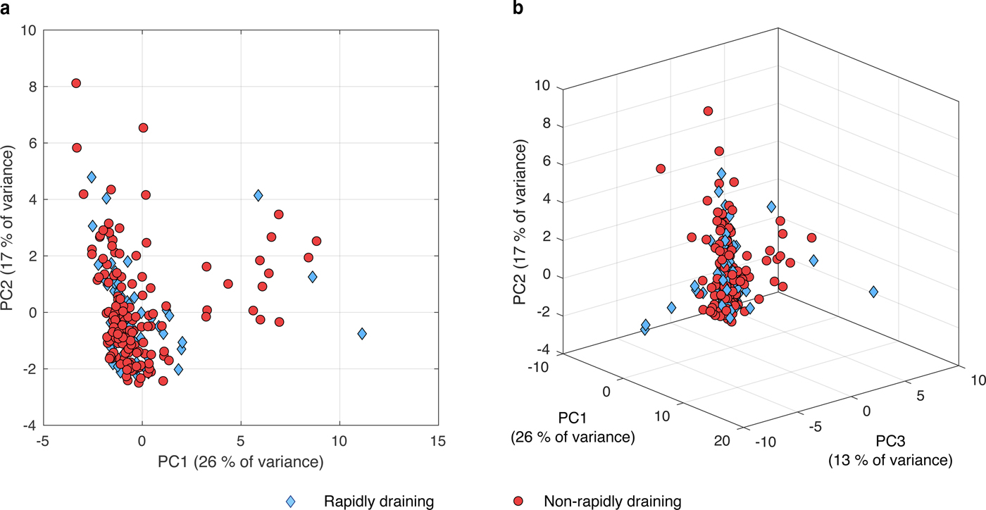
Fig. 9. PC scores for (a) PCs 1 and 2, and (b) PCs 1–3 for rapidly draining (blue diamonds) and non-rapidly draining (red circles) lakes for PCA conducted on all of the potential controlling factors (Table 2) included in the analysis (see Table S2 for eigenvectors). The percentage values labelled on the axes indicate the amount of variance in the data explained by each PC. The tight clustering of the rapidly draining and non-rapidly draining lake PC scores shows the statistical similarity of the potential controlling factors for the two lake types. For individual PCA plots for each category of potential controlling factor (Table 2), see Figures S5–S7.
Table 5. Results of unpaired Student's t-tests (for each category of controlling factor from Table 2, as well as for all of the 23 potential controlling factors simultaneously, shown within the ‘All’ category) for the rapidly draining and non-rapidly draining lakes scored for the first three PCs. None of the results are significant at above the 95% confidence interval (p < 0.05). See Table S2 for the eigenvectors for the first three PCs

3.3. Associations between lake area or volume and potential controlling factors
The fourth and final aim of the study was to determine whether there were differences in the associations between lake area or volume and the potential controlling factors for the two lake types, and whether there was a critical threshold for rapid lake drainage that could be linked to one of the other potential controlling factors. Existing modelling studies have only considered this possibility with regard to lake area or volume and the local ice thickness, but found similar model performance for a range of thresholds (Banwell and others, Reference Banwell2013, Reference Banwell, Arnold, Willis, Tedesco and Ahlstrøm2016; Arnold and others, Reference Arnold, Banwell and Willis2014; Koziol and others, Reference Koziol, Arnold, Pope and Colgan2017). It is plausible, however, that a lake area or volume threshold exists with respect to a factor other than local ice thickness. For example, hydrofracture might occur if a certain lake size is reached and a certain strain pattern exists (Fig. 7), with larger (or smaller) sizes required in more compressive (or more tensile) regions. Alternatively, perhaps rapid lake drainage is initiated once a certain lake size is attained and a particular volume of melt has already been lost from the catchment (Fig. 6), with larger (or smaller) lake sizes required in catchments where less (or more) melt has been lost into the GrIS. Bivariate correlations were examined between both lake areas (Table S3) and lake volumes (Table S4) and the other factors potentially controlling hydrofracture. The results in Tables S3 and S4 show that the majority of the correlations are statistically insignificant, indicating no link between these variables and lake area and volume. However, Table 6 presents results for the correlations that were statistically significant at above the 95% confidence interval. For rapidly draining lakes, the only significant correlation is between lake area and ice-bed elevation, but for the non-rapidly draining lakes there were more numerous significant correlations (Table 6). Tables S3 and S4 also show strong correlations between lake areas or volumes (for both rapidly draining and non-rapidly draining lakes) and the other hydrological factors, notably the maximum, mean and std dev. of lake depth, and the lake filling rate, but these are not included within Table 6 since it seems obvious that these variables should be correlated with lake area or volume.
Table 6. Statistically significant correlations identified between non-rapidly draining (NRD) and rapidly draining (RD) lake area or volume (the dependent variables) and the other potential controlling factors (the independent variables). Independent variables are labelled with their category of potentially controlling factor (see Table 2): glaciological (G), morphological (M) and SMB. ρ is the Spearman's rank correlation coefficient, with negative correlations highlighted in italicised font. p is the calculated probability, with all correlations shown significant at above the 95% confidence interval (i.e. p < 0.05) and those shown in bold text significant at above the 99% confidence interval (i.e. p < 0.01)

4. DISCUSSION
Collectively, our results show that rapidly draining and non-rapidly draining lakes for these two regions of the GrIS are largely indistinguishable in terms of the potential hydrofracture controlling factors examined here (Sections 3.1 and 3.2). This suggests that, in statistical terms, the lakes are drawn from the same population. Moreover, when the lakes are categorised according to their mode of drainage, the correlation analysis is unable to explain nearly all of the variability of lake area or volume for the rapidly draining lakes (except when ice-bed elevation was the independent variable), but can explain some of the variability for non-rapidly draining lakes (Section 3.3). Here, we first discuss the likely reasons for the results of the correlation analyses (Section 4.1); second, we examine the results of the statistical tests for difference for each category of potential controlling factor, with reference to existing hypotheses for rapid lake drainage (Section 4.2), and; finally, we discuss the potential explanations for the negative results of this study and suggest where future research should be directed (Section 4.3).
4.1. Associations between lake area or volume and potential controlling factors
When all of the lakes within both study regions were categorised according to their drainage mode, and then examined using a series of tests for correlation, the results indicate that, for rapidly draining lakes, the lakes normally drain before we observe that any of the controls are influential, whereas some of the controls are influential for the non-rapidly draining lakes. The negative weak correlation (Table 6) for both lake types between ice-bed elevation and lake area suggests that larger lakes tend to form in areas of lower ice-bed elevation, likely because the bed tends to be lower inland where the larger area lakes are present (Figs. 1 and 6). The weak positive correlation (Table 6) between ice thickness and non-rapidly draining lake area and volume can be explained because non-rapidly draining lakes grow bigger inland where the ice is thicker. This observation was also supported by the weak negative correlation (Table 6) between ice-surface slopes and non-rapidly draining lake volume since ice-surface slopes are lower inland (Fig. 5), meaning non-rapidly draining lakes can reach higher volumes here than closer to the coast, where the steeper ice-surface slopes prevent the formation of the largest lakes. These correlation results might also be because lakes tend to form over relatively low areas of bed topography (Lampkin and VanderBerg, Reference Lampkin and VanderBerg2011; Sergienko, Reference Sergienko2013). The lack of similar correlations between rapidly draining lake areas or volumes and the same factors indicates that ice thickness is not important in determining the size of the rapidly draining lakes prior to their drainage, instead suggesting that another factor may drive their rapid drainage. Non-rapidly draining lake volume also decreases as lakes become more eccentric (i.e. less circular and more linear; Fig. 5), and so the lakes will contain lower total water volumes, possibly because the more linear features occur higher on the ice sheet where lakes are bigger (Fig. 1), which could include some areas of slush rather than water contained within lakes. Finally, the correlation analysis shows that the cumulative totals of melt, rain and runoff in non-rapidly draining lake catchments are important in controlling the size of these lakes (Table 6), as we would expect. However, the lack of a similar relationship between these SMB factors and rapidly draining lakes may be because these factors are not important for affecting the size of these lakes.
4.2. Statistically similar rapidly draining and non-rapidly draining lakes
4.2.1. Hydrological factors
Among all factors examined, this category was the only one for which any difference between the two lake types was identified: non-rapidly draining lakes are, on average, more expansive than rapidly draining lakes (p < 0.05); with slightly reduced confidence (p = 0.054), they also contain larger water volumes. Existing models of the GrIS's hydrology use a critical threshold for lake area or volume, scaled with local ice thickness, to predict hydrofracture (Banwell and others, Reference Banwell2013, Reference Banwell, Arnold, Willis, Tedesco and Ahlstrøm2016; Arnold and others, Reference Arnold, Banwell and Willis2014; Clason and others, Reference Clason, Mair, Burgess and Nienow2015; Koziol and others, Reference Koziol, Arnold, Pope and Colgan2017). However, our results show that, in many places, non-rapidly draining lakes were able to expand without causing hydrofracture to a size that was larger than that which caused hydrofracture elsewhere. Thus, while these current models assume a certain lake area or volume triggers hydrofracture, which could indicate that rapidly draining lakes would be larger than non-rapidly draining lakes, our results point towards the opposite, showing that cause and effect may have been reversed. Here, we find that hydrofracture causes rapidly draining lakes to drain before they reach the larger sizes of the non-rapidly draining lakes. In addition, we find no correlation between rapidly draining lake area or volume and local ice thickness (although this correlation does exist for non-rapidly draining lakes), suggesting that rapidly draining lake area and volume do not scale according to ice thickness, but that the incidence of hydrofracture (presumably driven by a different control altogether) limits rapidly draining lake areas and volumes (Sections 3.3 and 4.1). These results agree with the lack of a direct relationship between the lake volume for rapidly draining lakes and the local ice thickness identified in previous work (e.g. Williamson and others, Reference Williamson, Arnold, Banwell and Willis2017; their fig. 15).
To examine this relationship further, we calculate the ‘fracture areas’, defined as the individual lake water volume divided by the local ice thickness, following Banwell and others (Reference Banwell2013, Reference Banwell, Arnold, Willis, Tedesco and Ahlstrøm2016) and Arnold and others (Reference Arnold, Banwell and Willis2014). We find that the fracture areas are higher for non-rapidly draining lakes than rapidly draining lakes: at Paakitsoq, the mean fracture area for rapidly draining lakes is 600 m2 (σ = 572 m2) compared with the mean fracture area for non-rapidly draining lakes of 2002 m2 (σ = 5084 m2); at Store Glacier, the mean fracture area for rapidly draining lakes is 663 m2 (σ = 594 m2) compared with a mean fracture area for non-rapidly draining lakes of 734 m2 (σ = 919 m2). These values show wide scatter across and between the study regions, supporting the idea that including a fracture area within models of the GrIS's surface hydrology is unlikely to be able to reproduce the precise locations and timings of rapid lake drainage, just their broad-scale patterns across the ice sheet (Arnold and others, Reference Arnold, Banwell and Willis2014).
While there is a difference between the rapidly draining and non-rapidly draining lake areas (p < 0.05) and volumes (p = 0.54) for the reasons explained above, the two lake types are statistically similar for the other hydrological factors (either individually or when combined into PCs). This indicates that the local, hydrological factors of individual lakes are unimportant in hydrofracture initiation. The fact that lake areas are significantly different between the two lake types, but lake volumes and depths are not (with 95% statistical confidence), may be due to the greater uncertainties associated with calculating lake water depth compared with lake area from MODIS imagery, possibly an effect of MODIS's coarse resolution. The FAST algorithm's depth-calculation method tends to report smaller values for the highest water depths compared with those derived from Landsat 8 imagery (Williamson and others, Reference Williamson, Arnold, Banwell and Willis2017). This might have resulted in the two lake types appearing statistically similar even though they were not. Using a finer-spatial resolution satellite record (such as the Sentinel-2 Multispectral Instrument (MSI), perhaps combined with Landsat 8 images) might overcome this issue, allowing a clearer conclusion to be reached on whether non-rapidly draining lakes, as well as covering larger areas and containing higher water volumes, also contain deeper water than rapidly draining lakes.
4.2.2. Morphological factors
The rapidly draining and non-rapidly draining lakes are similar in terms of their shapes and orientations, showing no link between these properties and the propensity for rapid lake drainage. This indicates that the distribution of the water load on the ice-sheet surface (i.e. whether it is more elongate or circular, and/or whether it is aligned more or less perpendicular or parallel to average ice-flow direction), is unimportant for hydrofracture initiation. This may be because the variation in load distribution is too small relative to the ice thickness to affect the hydrostatic-pressure potential, which possibly explains why we also find no statistically significant difference between the mean filling rates and the likelihood of hydrofracture.
4.2.3. Glaciological factors
Our results show that rapidly draining and non-rapidly draining lakes are similar in terms of the glaciological factors investigated. We included the long-term average winter stress field as a potential control on hydrofracture since higher temporal-resolution summer ice-velocity or strain-rate data were not available. While this was useful for defining the long-term average strain regime across each lake basin (which we hypothesised might be a first-order control on hydrofracture), we find no evidence that hydrofracture is controlled by the background winter stress or strain field. Existing research has only shown the degree of compression across a lake basin (e.g. Doyle and others, Reference Doyle2013), but has not considered whether the magnitude of the tensor affects the lake's likelihood of drainage, and we did not find support for this idea here. Moreover, we do not see that the background strain or velocity data scales with the rapidly draining lake areas or volumes (Section 3.3), suggesting that a threshold for rapidly draining lake area or volume cannot be linked to the local strain rate or ice velocity. Thus, we have no evidence that including the background stress regime in GrIS surface-hydrology models will improve their ability to predict rapid lake drainage. However, perhaps it is only the deviation from this long-term stress field that is important, resulting, for example, from surface meltwater reaching the bed via a nearby crevasse or moulin, perturbing the horizontal or vertical velocity or stress field beneath a lake basin (Stevens and others, Reference Stevens2015). We attempted to account for this process within our study by including the difference between the cumulative runoff in the lake's catchment and the lake's water volume, but also found negative results (Section 4.2.4).
4.2.4. SMB factors
Finally, the two lake types cannot be distinguished statistically on the basis of the SMB factors examined; we find no tendency for rapidly draining lakes to have different meltwater, rain and runoff quantities within their ice-surface catchments. The key rationale for including these factors was because previous work had found that water input to the ice-sheet bed nearby to a lake initiated hydrofracture (Stevens and others, Reference Stevens2015), so we used these SMB data as proxies for this process. Moreover, we specifically attempted to measure the input of water to the bed near to a lake by calculating the total melt in a lake's catchment minus the individual lake volume, but we find no support within our work for the lake-drainage mechanism observed by Stevens and others (Reference Stevens2015). However, we did observe a weak positive correlation between the melt, rain and runoff quantities and non-rapidly draining lake area and volume, even though the same correlations did not apply to rapidly draining lakes. This indicates that, for rapidly draining lakes, lake area and volume may not be dependent on these factors, or that they drain before the controls become manifest.
Even though we were unable to corroborate the findings of Stevens and others (Reference Stevens2015), that the input of water to the ice-sheet bed close to a lake is a precursor to hydrofracture, for a greater lake sample across the GrIS, this may reflect the coarse resolution of the MODIS imagery (250 m) and the RACMO2.3 grid (1 km) used in this study. The important meltwater-generation and surface-routing processes within lake catchments may operate at too fine a scale to be resolved with these data. Further studies that model or observe surface-meltwater production and its routing at spatial resolutions of metres to tens of metres and combine this information with ice-surface strain rates measured at hourly to daily temporal resolutions would be helpful for examining the influence of water delivery to the ice-sheet bed close to lakes in better detail. This objective could potentially be addressed using either higher-resolution remote-sensing imagery (e.g. WorldView, Sentinel-1 Synthetic Aperture Radar or Sentinel-2 MSI) or more field studies monitoring individual lakes and their catchments, which would generate data at a spatial resolution comparable with that of the size of a fracture formed by rapid lake drainage.
4.3. Reasons for this study's negative results and suggestions for future work
Here, we offer three explanations for which our study might not have found causal links between the potential controlling factors and hydrofracture, and suggest how these might be addressed with further research. First, although our EDA included many of the factors that we thought might be important in controlling hydrofracture (with the choice guided by previous research), other potential controls may have been overlooked. It is conceivable, therefore, that there is a control on hydrofracture that could be detected using our approach, but that we simply did not identify its potential at the outset. Alternatively, it is possible that a control is important but that it was not in summer 2014 within the study regions; further investigations for other sectors of the GrIS and in additional years would therefore help to validate our negative results. Second, the interplay between some of the controls that we did identify may be too complex to be elicited at the spatial and temporal scales used in this study. Remote sensing and SMB model outputs over finer grids and time steps may overcome this problem, or perhaps the control(s) might only be found from more field-based studies of individual or groups of lakes (Das and others, Reference Das2008; Doyle and others, Reference Doyle2013; Tedesco and others, Reference Tedesco2013; Stevens and others, Reference Stevens2015). With continuing improvements to the availability and resolution of remotely sensed data (such as ice-bed topography (e.g. Morlighem and others, Reference Morlighem, Rignot, Mouginot, Seroussi and Larour2017) or ice-velocity data), future studies that use a similar EDA approach to this one alongside these new datasets might be better able to reveal the control(s) on hydrofracture. Third, there may be a strong stochastic element to rapid lake drainage, which would explain the statistical similarity between the lake types observed in this study and which may help to explain why some lakes change their mode of drainage interannually (Selmes and others, Reference Selmes, Murray and James2013; Fitzpatrick and others, Reference Fitzpatrick2014). For example, hydrofracture might only be possible if pre-existing weaknesses exist in the ice beneath a lake basin, which can then be exploited by a load on the ice surface (Catania and others, Reference Catania, Neumann and Price2008). This would consequently make rapid lake drainage appear random. Without being able to include these very site-specific processes and ice-sheet features, which relate to the complex strain history up-glacier of a lake, it may be difficult to predict rapid lake drainage with confidence. A more detailed examination of such features as well as the strain history up-glacier of a lake would therefore be helpful.
5. CONCLUSIONS
Previous studies have suggested that rapid lake drainage is a key contributor to the GrIS's negative mass balance and may become more widespread in the future as lakes continue to advance inland. Despite this, the precise controls on rapid lake drainage remain uncertain, having not been examined comprehensively within existing research. Our aim here was therefore to address this shortfall by conducting a comprehensive, statistically robust EDA of various potential controls on hydrofracture for a large sample of rapidly draining and non-rapidly draining lakes in West Greenland.
Our results, however, did not indicate any clear links between the incidence of hydrofracture and the potential controlling factors examined for the two study regions in summer 2014. This means that we cannot recommend an empirically supported alternative to the fracture area threshold parameter in use within current surface-hydrology models of the GrIS (Banwell and others, Reference Banwell2013, Reference Banwell, Arnold, Willis, Tedesco and Ahlstrøm2016; Arnold and others, Reference Arnold, Banwell and Willis2014; Clason and others, Reference Clason, Mair, Burgess and Nienow2015; Koziol and others, Reference Koziol, Arnold, Pope and Colgan2017), but nor can we provide evidence to support the use of a fracture area threshold parameter in future surface-hydrology models if the aim is to predict the precise magnitude and timing of individual rapid lake-drainage events. Here, we showed that rapid lake drainage controls lake size, and not the reverse, directly contradicting the use of a fracture area threshold in such models. Using a deterministic basis to predict precisely when and where rapid lake drainage will occur therefore remains the weakest component of GrIS hydrology models, despite recent work showing the importance of the lake-drainage process for the evolution of subglacial drainage (Banwell and others, Reference Banwell, Arnold, Willis, Tedesco and Ahlstrøm2016). Future work could focus on incorporating some of the potential controls identified here into supraglacial-hydrology models of the GrIS, and testing their ability to reproduce empirical observations with these controls included. These improvements to surface-hydrology models are necessary to provide more realistic inputs to SMB models (requiring knowledge of lake locations and their duration on the GrIS surface to determine the amount of enhanced surface ablation), and to coupled subglacial hydrology-ice flow models (requiring knowledge of the timing and magnitude of meltwater deliveries to the ice-sheet bed to determine ice-dynamic impacts). Therefore, if better knowledge were gained of the controls on the hydrofracture process, these deterministic models could be confidently forced with future climate projections; this would generate robust patterns of rapid lake drainage across the GrIS, ultimately helping to improve forecasts of water runoff, dynamic ice discharge and thus sea-level rise from the GrIS over the coming century.
AUTHOR CONTRIBUTIONS
All authors conceived the study. AGW designed the methodological approach, processed the data and undertook the analysis under supervision from the other authors. All authors were involved in interpreting the results. AGW wrote the manuscript, with all authors commenting on and editing it. AGW, with input from ICW, revised the manuscript following reviewer and editorial comments.
SUPPLEMENTARY MATERIAL
The supplementary material for this article can be found at https://doi.org/10.1017/jog.2018.8
ACKNOWLEDGEMENTS
AGW was funded by a UK Natural Environment Research Council PhD studentship (NE/L002507/1) awarded through the Cambridge Earth System Science Doctoral Training Partnership. AFB was funded by a Leverhulme/Newton Trust Early Career Fellowship (ECF-2014-412). We thank Brice Noël for providing the RACMO2.3 data, and Conrad Koziol for providing the original MATLAB function to calculate the von Mises yield criterion from the ice-velocity data. We are grateful to Nick Selmes for discussions during the conception of the study, and to Jerome Neufeld and Stephen Kissler for their early advice regarding the appropriate statistical techniques for the research. Finally, we thank Ted Scambos (the Scientific Editor) and one anonymous reviewer for their comments that improved the manuscript.


 Open access