


1. INTRODUCTION
An understanding of the physical processes that take place within glaciers requires information about the plastic deformation behavior of ice at high pressures. Jones and Chew (Reference Jones and Chew1983) and Mctigue and others (Reference Mctigue, Passman and Jones1985) reported creep experiments on polycrystalline ice subject to a combination of uniaxial compression and hydrostatic pressure. Further, Barrette and Jordaan (Reference Barrette and Jordaan2003) investigated the compressive behavior of laboratory-produced ice as well as genuine iceberg ice subjected to constant confinement pressure.
Passman (Reference Passman1982) obtained an exact solution for the deformation in biaxial creep tests using the constitutive equation of a second-grade fluid. In his model, there are three constant constitutive parameters (including the viscosity). Mctigue and others (Reference Mctigue, Passman and Jones1985) showed that these constitutive parameters exhibit a non-negligible dependence on the applied hydrostatic pressure (the confining pressure). They ascribed this phenomenon to a partial inadequacy of the second-grade fluid model. They stated ‘The results presented here, then, are not intended to suggest that the second-order fluid model gives a complete representation for the behavior of ice.’
The fact that the ice parameters (obtained by fitting the experimental data) show significantly different values at different pressures were also emphasized by Jones and Chew (Reference Jones and Chew1983), who wrote ‘It has always been assumed that the application of hydrostatic pressure increases the creep rate of ice.’This effect was noticed for the first time by Rigsby (Reference Rigsby1958), who stated: ‘the shear strain rate increased as the pressure was increased at constant temperature, but that rate is practically independent of hydrostatic pressure when the difference between the ice temperature and the melting temperature is kept constant.’
Barrette and Jordaan (Reference Barrette and Jordaan2003) reported a number of experimental tests, designed to investigate the deformation of ice under a constant compressive load and at various confinement pressures. In particular, the testing conditions (confinements and axial stress) are thought to be representative of those that can occur in interactions between icebergs and engineered structures, such as the hull of a ship. Despite such experimental evidence, few theoretical explanations have been proposed so far; see Glen (Reference Glen1955), Van Der Veen (Reference Van Der Veen2013), Section 6.2 of Schulson and Duval (Reference Schulson and Duval2009); Greve and others (Reference Greve, Zwinger and Gong2014).
Recently, Rajagopal (Reference Rajagopal2003, Reference Rajagopal2006) argued that it is often advantageous to write constitutive relations in implicit forms. In this perspective, the material parameters characterizing the constitutive model can depend on the stress itself and therefore also on the pressure (the latter being the trace of the Cauchy stress tensor, Rajagopal (Reference Rajagopal2015)).
Our purpose is to propose two models that can explain the experimental results concerning primary creep (or transient creep) and secondary creep (Jones and Chew (Reference Jones and Chew1983); Mctigue and others (Reference Mctigue, Passman and Jones1985); Barrette and Jordaan (Reference Barrette and Jordaan2003)), which include a rheology depending significantly upon the pressure. This fact can be observed in Figure 3 of Barrette and Jordaan (Reference Barrette and Jordaan2003) or in Figure 2 of Mctigue and others (Reference Mctigue, Passman and Jones1985), where the effect of the pressure on the rheological behavior of ice becomes evident. Thus, starting from the second-grade fluid model, we consider two constitutive equations in which we add the fundamental hypothesis that the rheological parameters depend on the pressure. We select the second-grade fluid model because it is known that this model can represent primary and secondary (but not tertiary) creep (Passman (Reference Passman1982)), while a power-law model can represent only secondary creep.
The proposed models are based on (i) an equation which generalizes the classical second grade constitutive equation (Mctigue and others (Reference Mctigue, Passman and Jones1985)), and (ii) an equation which is a generalization of a power-law fluid of grade 2 (Man and Sun (Reference Man and Sun1987)). Model (i) is a generalization of the simplest fluid model of differential type that can capture normal stress differences. However, since second-grade models usually fail to represent the non-linear rate dependence of ice in shear (Mctigue and others (Reference Mctigue, Passman and Jones1985); Man and Sun (Reference Man and Sun1987)) we also consider model (ii) that accounts for both shear thinning (as in Glen's law) and normal stress differences.
We believe that (i) and (ii) are improvements on the models of Mctigue and others (Reference Mctigue, Passman and Jones1985) and Man and Sun (Reference Man and Sun1987) because, given the high pressures that develop within glaciers, we expect the viscosity to depend also on the pressure (as experimentally highlighted by Jones and Chew (Reference Jones and Chew1983), Mctigue and others (Reference Mctigue, Passman and Jones1985) and Barrette and Jordaan (Reference Barrette and Jordaan2003)). The dependence of the viscosity on the pressure is indeed a well-known phenomenon (see, for instance, Bridgman (Reference Bridgman1958) for a discussion of the early experimental work concerning the dependence of viscosity on pressure). Further, models (i) and (ii) can generate normal stress effects. This phenomenon was highlighted by Mctigue and others (Reference Mctigue, Passman and Jones1985) and Man and Sun (Reference Man and Sun1987), where the free-surface depression of a second-grade fluid flowing down an inclined open semi-circular channel is estimated.
In this paper, we analyze the one-dimensional (1-D) flow experienced by ice samples during a creep test, assuming that the rheological parameters follow a Barus-type lawFootnote 1 (Barus (Reference Barus1893); Bridgman (Reference Bridgman1958); Szeri (Reference Szeri2005)). The specific choice of the Barus law is mainly guided by empiricism and the requirement of simplicity. We present a similar analysis for both models (i) and (ii), showing how the dependence of the rheological parameters on pressure has non-negligible qualitative and quantitative effects on the flow. Actually, both models describe quite well the experimental results presented in Jones and Chew (Reference Jones and Chew1983), Mctigue and others (Reference Mctigue, Passman and Jones1985) and Barrette and Jordaan (Reference Barrette and Jordaan2003), and capture the increase in the creep rate caused by the increasing pressure.
The paper is organized as follows: in the first section, we present models (i) and (ii). In the second section, the governing equations for creep flow are derived. In the third section, we illustrate the fitting of the parameters against the experimental data relating to primary and secondary creep. The last section is devoted to some concluding remarks.
2. THE MODEL
We consider a class of constitutive equations originating from the second-grade fluid model of implicit type (Rajagopal (Reference Rajagopal2003, Reference Rajagopal2006); Rajagopal and Szeri (Reference Rajagopal and Szeri2003)) of the form
 $$f\left( {{\bf T},{\bf A}_1,{\bf A}_2, \ldots ,{\bf A}_n} \right) = 0,$$
where T is the Cauchy stress tensor and An are the Rivlin-Ericksen tensors (Passman (Reference Passman1982); Truesdell and Rajagopal (Reference Truesdell and Rajagopal2000))
 $${\bf A}_1 = \left( {\nabla {\bf v} + \nabla {\bf v}^{\rm T}} \right) = {\bf G} + {\bf G}^{\rm T},$$
 $${\bf A}_2 = \displaystyle{{{\rm d}{\bf A}_1} \over {{\rm d}t}} + {\bf A}_1{\bf G} + {\bf G}^{\rm T}{\bf A}_1,$$
 $${\bf A}_n = \displaystyle{{{\rm d}{\bf A}_{n-1}} \over {{\rm d}t}} + {\bf A}_{n-1}{\bf G} + {\bf G}^{\rm T}{\bf A}_{n-1}.$$
The tensor G in Eqns (2)–(4) denotes the gradient of the velocity field v(x,t), i.e.  $\nabla {\bi v}= {\bf G}$. In particular, ${\bf G} = \dot{{\bf F}}{\bf F}^{-1}$ where F is the deformation gradient tensor.
We assume mechanical incompressibility so that
 $${\rm tr}{\bf A}_1 = 0.$$
2.1. Second-grade fluid type constitutive models
We select second-grade fluids (Truesdell and Rajagopal (Reference Truesdell and Rajagopal2000)) because Mctigue and others (Reference Mctigue, Passman and Jones1985) show that these models give an excellent representation of primary creep of ice at constant confining pressure. More importantly, Truesdell and Noll (Reference Truesdell and Noll1992) show that second-grade fluids exhibit normal stress differences, a feature which power-law constitutive models cannot capture and which seems to play a significant role in ice deformation.
As the first constitutive model, we generalize the basic second-grade fluid model proposed in Mctigue and others (Reference Mctigue, Passman and Jones1985), assuming that the characteristic constitutive parameters depend on the pressure p, the mean normal stress (Rajagopal and others (Reference Rajagopal, Saccomandi and Vergori2012, Reference Rajagopal, Saccomandi and Vergori2015); Rajagopal (Reference Rajagopal2015); Rajagopal and Saccomandi (Reference Rajagopal and Saccomandi2016)):
 $$p = -\displaystyle{1 \over 3}{\rm tr}{\bf T}\; .$$
We thus considerFootnote 2
 $$\eqalign{{\bf T} & = -p{\bf I} + \mu \left( p \right){\bf A}_1 + \alpha _1\left( p \right)\left[ {{\bf A}_2-\displaystyle{1 \over 3}({\rm tr }{\bf A}_2){\bf I}} \right] + \alpha _2(\,p) \cr & \times \left[ {{\bf A}_1^2 -\displaystyle{1 \over 3}({\rm tr}{\bf A}_1^2 ){\bf I}} \right]},$$
where tr(T + p I) = 0. As stated earlier, we assume that the coefficients characterizing the constitutive Eqn (6) of the fluid may depend on p so that the constitutive model is implicit. Such an assumption, as we shall see, plays a key role in the analysis of the flow.
Next, we impose the following restrictions on the constitutive parameters:
 $$\mu \geq 0, \quad \alpha _{1}<0, \quad \alpha _{1}+\alpha _{2}\neq 0,$$
which are suggested by some experiments performed on polymer solutions and melts (Bird and others (Reference Bird, Amstrong and Hassager1977)). Using thermodynamic arguments, Dunn and Fosdick (Reference Dunn and Fosdick1974) showed that α1 ≥ 0 and α2 + α1 = 0. In particular, if α1 is positive the Clausius-Duhem inequality is met and the Helmholtz potential is a minimum when the fluid is at rest. Fosdick and Rajagopal (Reference Fosdick and Rajagopal1979) showed that, irrespectively of the sign of α1 + α2, the fluid model exhibits unacceptable stability characteristics when α1 is negative. We refer to Dunn and Rajagopal (Reference Dunn and Rajagopal1995) for a detailed discussion on the relevant issues concerning second-grade fluids. These restrictions, however, need not be straightforwardly applicable to our models, since we are considering implicit constitutive equations. Indeed, referring to Fosdick and Rajagopal (Reference Fosdick and Rajagopal1979), we remark that their results are obtained by using a relation involving an L 2 estimate of v, ‖A1‖ and an L 1 estimate of  $$\left\Vert {{\bf A}_1} \right\Vert^3$$, in which the material moduli μ, α1 and α2 are taken constant. Such an approach is no longer applicable in our case since the material moduli depend on the stress itself. In other words, the separation between kinematic variables and stress (on which the procedure developed in Fosdick and Rajagopal (Reference Fosdick and Rajagopal1979) is based) cannot be performed in our case. Therefore, following Mctigue and others (Reference Mctigue, Passman and Jones1985), assumptions (7) are essentially based on experimental evidence.
As a second constitutive model, we consider a generalized version of the one proposed by Man and Sun (Reference Man and Sun1987):
 $$\eqalign{&{\bf T} = -p{\bf I} + \mu \left( p \right)\left[ {a_0 + \displaystyle{1 \over 2}({\rm tr}\,{\bf A}_1^2 )} \right]^{m/2}{\bf A}_1 + \alpha _1(\,p) \cr & \times \left[ {{\bf A}_2-\displaystyle{1 \over 3}({\rm tr}\,{\bf A}_2){\bf I}} \right] + \alpha _2(\,p)\left[ {{\bf A}_1^2 -\displaystyle{1 \over 3}({\rm tr}\,{\bf A}_1^2 ){\bf I}} \right]},$$
where a 0 and m are constants which depend on the nature of the ice. Following Kannan and Rajagopal (Reference Kannan and Rajagopal2013), we consider m = −(2/3) and a 0 = 0, but here we assume that the restrictions (7) hold true.
We consider the constitutive Eqn (8) because it is a simple model exhibiting both normal stress differences and shear thinning effects, which agrees with the power law proposed by Glen (Reference Glen1955). In fact, some experimental results clearly indicate that glacier ice shows shear thinning (Kjartanson and others (Reference Kjartanson, Shields, Domaschuk and Man1988)). In a sense, our approach is parallel to the one presented by Man and Sun (Reference Man and Sun1987), where the creep data of Mctigue and others (Reference Mctigue, Passman and Jones1985) were used to determine the material parameters.
Before proceeding further, we emphasize that, in general, the second-grade fluid model gives rise to considerable mathematical issues. Indeed, the related mathematical problems involve derivatives of third order, i.e. one order higher than in the Navier-Stokes equation. Therefore, when considering fully 3-D flows, one needs additional boundary conditions (Rajagopal and Kaloni (Reference Rajagopal, Kaloni, Graham and Malik1989); Rajagopal (Reference Rajagopal and Sequeira1995)). However, this problem can be circumvented when the constitutive model is written in an implicit form. Indeed, the constitutive relation is solved together with the balance of linear momentum, without substituting the expression for the stress into the balance of linear momentum. So the order of the differential equations is not increased and no further boundary conditions are needed. Clearly, such a procedure works also when the material coefficients are constant. We refer the readers to Rajagopal (Reference Kjartanson, Shields, Domaschuk and Man2003) where this issue is discussed at length.
Concerning the dependence on p of the parameters μ and α2, we consider a Barus-type law (Barus (Reference Barus1893); Bridgman (Reference Bridgman1958)), while α1 is assumed not to depend on p:
 $$\mu (\,p) = \mu _0{\rm exp}\left( {-k_\mu \displaystyle{{\,p-p_{{\rm ref}}} \over {\,p_{{\rm ref}}}}} \right),$$
 $$\alpha _2(\,p) = \alpha _{2,0}{\rm exp}\left( {-k_\alpha \displaystyle{{\,p-p_{{\rm ref}}} \over {\,p_{{\rm ref}}}}} \right),$$
 $$\alpha _1 = {\rm constant}\;{\rm with}\;{\rm respect}\;{\rm to}\;{\rm the}\;{\rm pressure}\;p,$$
with μ 0, α 2,0, k μ and k α constants and where p ref is a reference pressure.
For (9), we selected a Barus-type law simply because it gives a good fit in many contexts. For instance, we find an exponential variation in the viscosity due to pressure in problems such as elastohydrodynamics (Szeri (Reference Szeri2005)), in problems involving the flow of geological matter (Sahaphol and Miura (Reference Sahaphol and Miura2005)), and the response of composite materials (Shin and Pae (Reference Shin and Pae1992)). The properties of polymeric materials may also vary exponentially with pressure (Jones Parry and Tabor (Reference Jones Parry and Tabor1973)). We, however, remark that, to our knowledge, there are no experiments showing that the ice viscosity varies exponentially with pressure.
The issue of pressure-dependent viscosity is also analyzed by Kannan and Rajagopal (Reference Kannan and Rajagopal2013), who propose a model that takes into account both the pressure and the volume fraction of the rock sands and grains trapped within the interstices of the rock glacier. Our context is different: we consider experiments performed on a sample of polycrystalline ice with no impurities trapped inside.
Assumption (10) is new since there are no theoretical or experimental studies suggesting it. The choice of this law is inspired by the rheology of some organic liquids.
Finally, we assume (11) following Kannan and Rajagopal (Reference Kannan and Rajagopal2013). Actually, in fitting the experimental data, we found that α1 is practically insensitive to the pressure variations (at least in the range of the considered data).
3. CREEP FLOW
We consider a sample of polycrystalline ice and select a Cartesian coordinate system. The sample has length l 0 in the undeformed reference configuration (see Fig. 1a). We then consider an isochoric homogeneous flow (elongational or compression flow) as in creep flow tests (see Fig. 1b), where l(t) denotes the sample length at time t, and
 $$\beta (t) = \displaystyle{{l(t)} \over {l_0}}$$
is the stretch. Obviously β(t) is related to the axial strain ε(t) = (l(t) − l 0)/l 0 by β(t) = ε(t) + 1. We also introduce the strain rateFootnote 3  $\dot {\epsilon }=\dot {\beta }$, i.e. the change in deformation with respect to time.
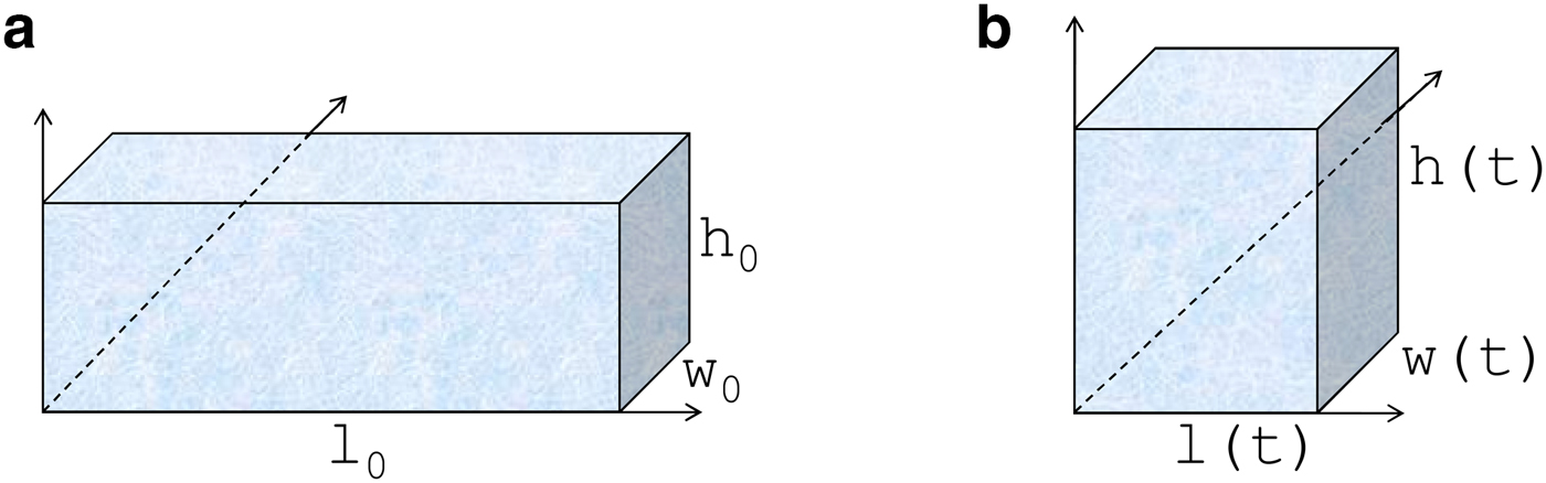
Fig. 1. Reference and current configuration.
Proceeding as in Passman (Reference Passman1982) and Mctigue and others (Reference Mctigue, Passman and Jones1985), the deformation gradient tensor is diagonal and has the formFootnote 4
 $${\bf F} = {\rm diag}\left[ {\beta (t),\displaystyle{1 \over {\sqrt {\beta (t)} }},\displaystyle{1 \over {\sqrt {\beta (t)} }}} \right],$$
while the Rivlin-Ericksen tensors A1, A2 take the diagonal forms
 $${\bf A}_1 = {\rm diag}\left[ {2a,\; -a,\; -a} \right],$$
 $${\bf A}_2 = {\rm diag}[2\dot{a} + 4a^2,\; -\dot{a} + a^2,\; -\dot{a} + a^2],$$
where
 $$a\left( t \right) = \displaystyle{{\dot{\beta }\left( t \right)} \over {\beta \left( t \right)}}.$$
For the Cauchy stress tensor, we have
 $${\bf T} = {\rm diag}[\,f_A(t),\; f_L(t),\; f_L(t)],$$
where f A(t) is the stress along the x-axis (axial stress) and f L(t) is the lateral stress, also referred to as confining pressure (Jones and Chew (Reference Jones and Chew1983); Mctigue and others (Reference Mctigue, Passman and Jones1985)). The loads are portrayed in Fig. 2.
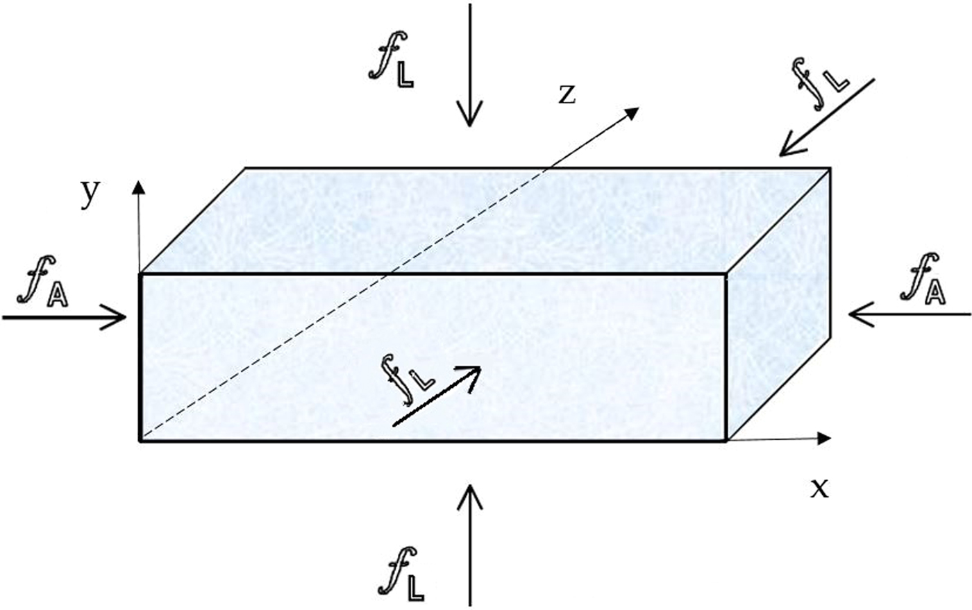
Fig. 2. A sample subjected to a compressive force f A and a confining pressure f L.
Applying the stress equilibrium equation and the model (6), we obtain the differential equation
 $$ f_{A}-f_{L}=3a\mu \left( p\right) +3\alpha _{1}\dot{a}+3a^{2}(\alpha _{1}+\alpha _{2}\left( p\right) ),$$
with the initial condition a(0) = a 0.
The pressure is given by
 $$p = -\displaystyle{1 \over 3}\left[ {\,f_A + 2f_L} \right].$$
Following Passman (Reference Passman1982) and assuming that f A, f L are constant in time, Eqn (15) can be solved analytically. To see this, we introduce the following parameters
 $$\nu \left( p \right) = \displaystyle{{\mu \left( p \right)} \over {2\left( {\alpha _1 + \alpha _2\left( p \right)} \right)}},$$
 $$\chi \left( p \right) = 1 + \displaystyle{{\alpha _2\left( p \right)} \over {\alpha _1}},$$
 $$b^2\left( p \right) = \displaystyle{{\mu ^2\left( p \right)} \over {4{(\alpha _1 + \alpha _2\left( p \right))}^2}} + \displaystyle{{\,f_A-f_L} \over {3\left( {\alpha _1 + \alpha _2\left( p \right)} \right)}},$$
which, unlike in Passman (Reference Passman1982), depend on p because of (9) and (10).
Equation (15) coincides with equation (29) of Passman (Reference Passman1982). We can solve it analytically because both f A and f L are constant in time. The solution procedure is equal to the one illustrated by Passman (Reference Passman1982). Indeed, since p does not change in time, the parameters in (15) are constant. Therefore we keep the main result of Passman (Reference Passman1982), limiting our discussion to the case b 2 > 0. The latter yields physically reasonable results and provides the best fits to laboratory creep data, as shown by Passman (Reference Passman1982) and Mctigue and others (Reference Mctigue, Passman and Jones1985). We will check a posteriori that the assumption b 2 > 0 is actually fulfilled, at least in the considered range of pressures. Of course, outside this range, it could happen that b 2 becomes negative, simply because
 $$f_A-f_L < -\displaystyle{{3\mu ^2\left( p \right)} \over {4\left( {\alpha _1 + \alpha _2\left( p \right)} \right)}}.$$
Should this occur, then there would be a critical time at which the deformation rate and the strain become undefined. This fact does not mean that the model fails, but that homogeneous deformations do not exist anymore.
So, considering b 2 > 0, we obtain
 $$\displaystyle{{a(t) + \nu } \over b} = \displaystyle{{\left[ {\left( {a_0 + \nu } \right)/b} \right]\cosh \left( {\chi bt} \right) + \sinh \left( {\chi bt} \right)} \over {\left[ {\left( {a_0 + \nu } \right)/b} \right]\sinh \left( {\chi lt} \right) + \cosh \left( {\chi bt} \right)}},$$
and
 $${\epsilon }(t) = \beta _0\left[ {\cosh \left( {\chi bt} \right) + \left( {\displaystyle{{a_0 + \nu } \over b}} \right)\sinh \left( {\chi bt} \right)} \right]^{1 \over \chi }{\displaystyle}{\rm e}^{-\nu t}-1,$$
β0 being the initial stretch.
If instead of the constitutive model (6) we consider (8) with m = −2/3 and a o = 0, we obtain the differential equation:
 $$\dot{a} = -\lambda \left( p \right)a^{1/3} + \chi \left( p \right)a^2 + c\left( p \right),$$
where
 $$\lambda (\,p) = \root 3 \of {\displaystyle{1 \over 3}} \displaystyle{{\mu (\,p)} \over {\alpha _1(\,p)}},\quad c(\,p) = \displaystyle{{\,f_A-f_L} \over {3\alpha _1(\,p)}}.$$
Equation (19) is solved numerically assuming that f A and f L are constant in time.
4. FITTING OF THE PARAMETERS WITH EXPERIMENTAL DATA
In order to validate the models (6) and (8), along with the assumptions (9)–(11), we consider the experimental data reported in Jones and Chew (Reference Jones and Chew1983), Mctigue and others (Reference Mctigue, Passman and Jones1985) and Barrette and Jordaan (Reference Barrette and Jordaan2003), which refer to a series of creep flow tests performed on polycrystalline ice samples, maintained at constant temperature, at different confinement pressures.
First, we focus on the data shown by Mctigue and others (Reference Mctigue, Passman and Jones1985) and Jones and Chew (Reference Jones and Chew1983) since they are the same experimental data but presented in different forms. Then we analyze the experimental data of Barrette and Jordaan (Reference Barrette and Jordaan2003). So, starting with Mctigue and others (Reference Mctigue, Passman and Jones1985) and Jones and Chew (Reference Jones and Chew1983), we denote by:
1. the data analysis presented in Mctigue and others (Reference Mctigue, Passman and Jones1985),
2. the data analysis illustrated in Jones and Chew (Reference Jones and Chew1983).
In particular, data analysis 2 consists essentially of the creep curves shown in Figure 1 of Jones and Chew (Reference Jones and Chew1983), where the strain rate is plotted against strain under different confining pressures: 0 and 50 MPa. The difference between the two curves is obvious, meaning that the rheological properties of ice are different at different pressures, as remarked by Jones and Chew (Reference Jones and Chew1983).
Data analysis 1 refers to Figure 2 of Mctigue and others (Reference Mctigue, Passman and Jones1985), which displays the axial strain vs. time corresponding to three different confining pressures: atmospheric pressure, 37 and 50 MPa. Also, in this case, the slopes of the curves increase with pressure. The first and last curves differ by a factor ~ 2.
The five parameters μ0, k μ, α2,~0, k α, α1 characterizing (18) and the differential Eqn (19) are obtained by fitting to the experimental data. Since the data refer to the same experiments, we have fitted the coefficients by considering analyses 1 and 2 separately. By comparing the results obtained, we are able to evaluate the validity of the proposed models.
The outcomes of the best-fit procedures (whose details are not shown here) are summarized in Tables 1 (data analysis 1) and 2 (data analysis 2), where (a) refers to equation (18), i.e. model (6), and (b) refers to equation (19), i.e. model (8).
Table 1. Constitutive coefficients and pressures for creep tests, obtained by fitting to the experimental data of Mctigue and others (Reference Mctigue, Passman and Jones1985)
Table 2. Constitutive coefficients and pressures for creep tests, obtained by fitting to the experimental data of Jones and Chew (Reference Jones and Chew1983)
In Table 1a we report the values of the coefficients μ 0, k μ, α 2,~0, k α, α 1, obtained by fitting the axial strain ε(t) given by (16) to the data analysis 1, while Table 1b shows the same five parameters obtained by fitting ε(t) given by (19).
The coefficients of Tables 1a and 2a are similar, with differences being of the order 15–20%. This observation strengthens model (6) since we obtain very similar values for the rheological parameters. By contrast, the coefficients of Tables 1b and 2b differ more from each other. In particular, we note a significant difference in k α.
The fittings are shown graphically in Figs 3–6. Figures 3 and 4 refer to ε(t) given by equation (18), i.e. the constitutive model (6). In Fig. 3 we plot the data analysis illustrated in Mctigue and others (Reference Mctigue, Passman and Jones1985) (circles), and the axial strain ε(t) computed with the coefficients of Table 1. Figure 4 shows ε vs.  $\dot {\epsilon }$, computed with μ 0, k μ, α 2,~0, k α, α 1 of Table 2a and the data of Jones and Chew (Reference Jones and Chew1983) (circles). Figures 5 and 6 refer to equation (19) (constitutive model (8)). Figure 5 shows the comparison with the analysis of Mctigue and others (Reference Mctigue, Passman and Jones1985), and Fig. 6 displays the data by Jones and Chew (Reference Jones and Chew1983) (circles) and $\epsilon ,\,\dot {\epsilon }$, computed using the parameters of Table 2b.
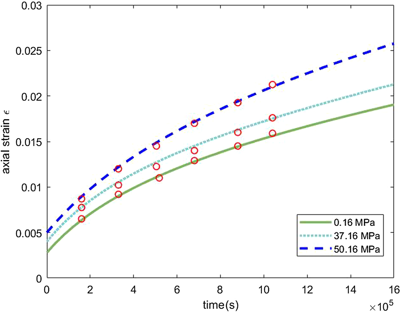
Fig. 3. Axial strain vs. time for different confining pressures, computed with model (6) and the coefficients of Table 1. Experimental data (small circles) of Mctigue and others (Reference Mctigue, Passman and Jones1985).
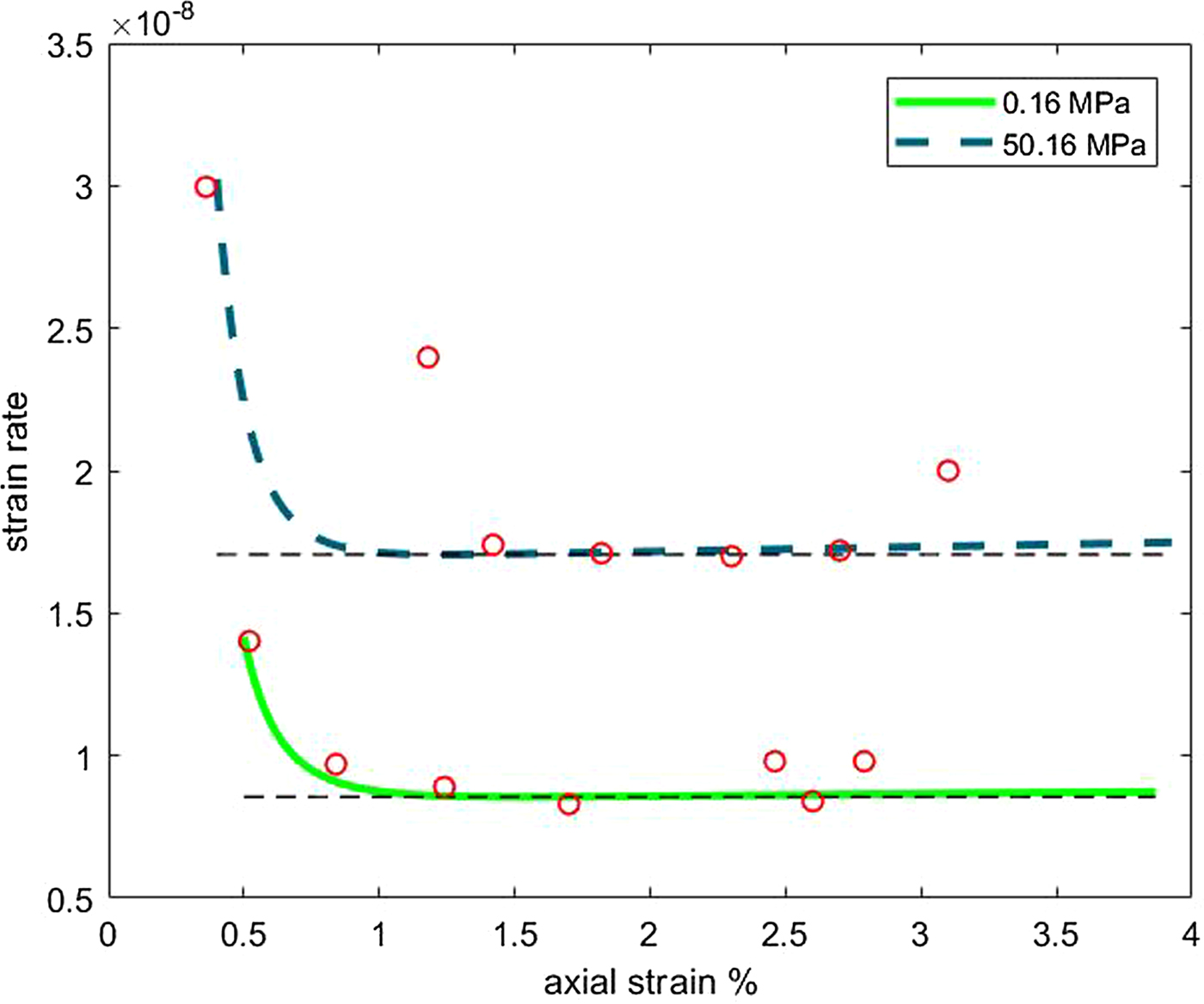
Fig. 4. Strain rate vs. axial strain for different confining pressures, computed with model (6) and the coefficients of Table 2. Experimental data (small circles) of Jones and Chew (Reference Jones and Chew1983).

Fig. 5. Axial strain vs. time at different confining pressures, computed with model (8) and the coefficients of Table 1b. Experimental data (small circles) of Mctigue and others (Reference Mctigue, Passman and Jones1985).
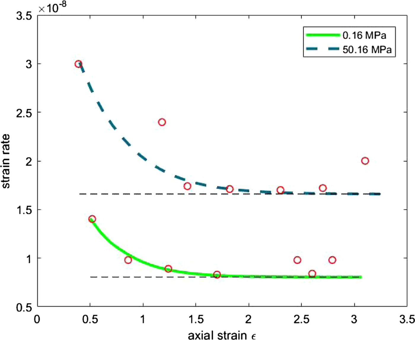
Fig. 6. Strain rate vs. axial strain at different confining pressures, computed with model (8) and the coefficients of Table 2b. Experimental data (small circles) of Jones and Chew (Reference Jones and Chew1983).
A second set of experimental data, independent of those reported by Mctigue and others (Reference Mctigue, Passman and Jones1985) and Jones and Chew (Reference Jones and Chew1983), is shown in Figure 3 of Barrette and Jordaan (Reference Barrette and Jordaan2003). These data reveal the onset of tertiary creep for longer times. However, for the purpose of fitting models (6) and (8), the data are truncated at the onset of tertiary creep. The coefficients obtained by fitting the three curves reported in Fig. 3 of Barrette and Jordaan (Reference Barrette and Jordaan2003) are listed in Tables 3a and 3b. Now the axial stress f A is f L + 15MPa, while in Mctigue and others (Reference Mctigue, Passman and Jones1985) and Jones and Chew (Reference Jones and Chew1983) f A = f L + 0.47MPa. Moreover, the order of magnitude of strain rate is ~105 times larger than that of Mctigue and others (Reference Mctigue, Passman and Jones1985) and Jones and Chew (Reference Jones and Chew1983).
Table 3. Constitutive coefficients and pressures for creep tests, obtained by fitting to the experimental data of Barrette and Jordaan (Reference Barrette and Jordaan2003)
The fitted curves are shown in Figs 7 and 8. In particular, Fig. 7 displays the comparison between the data by Barrette and Jordaan (Reference Barrette and Jordaan2003) and the model (6), while Fig. 8 shows the comparison with model (8). Actually, both models reproduce quite well the primary and secondary creep stages.
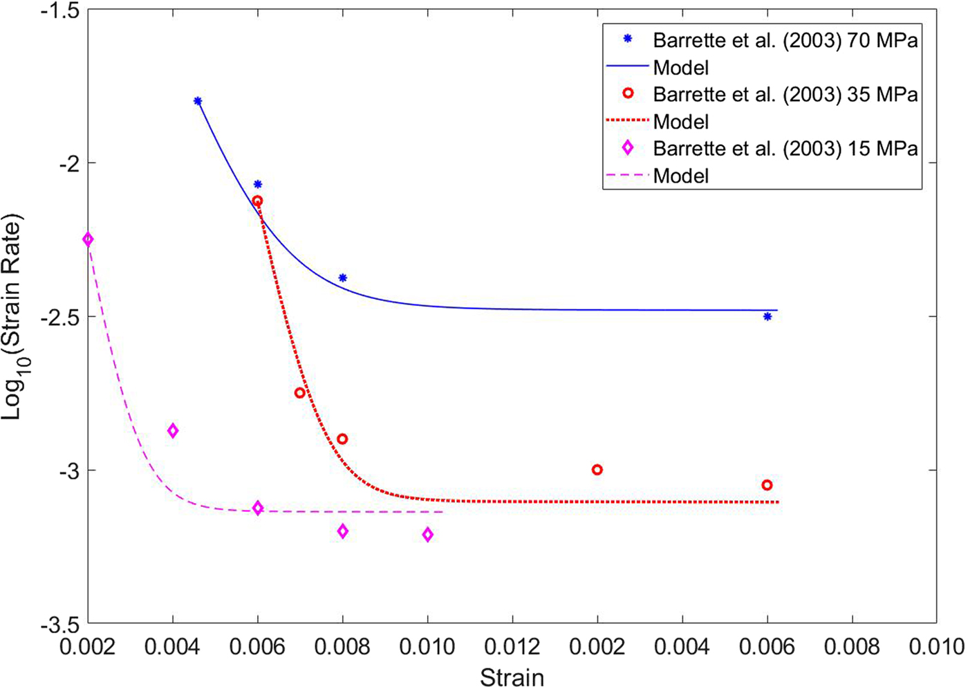
Fig. 7. Strain rate vs. axial strain at different confining pressures, computed with model (6) and the coefficients of Table 3a. Experimental data (small circles) of Barrette and Jordaan (Reference Barrette and Jordaan2003).
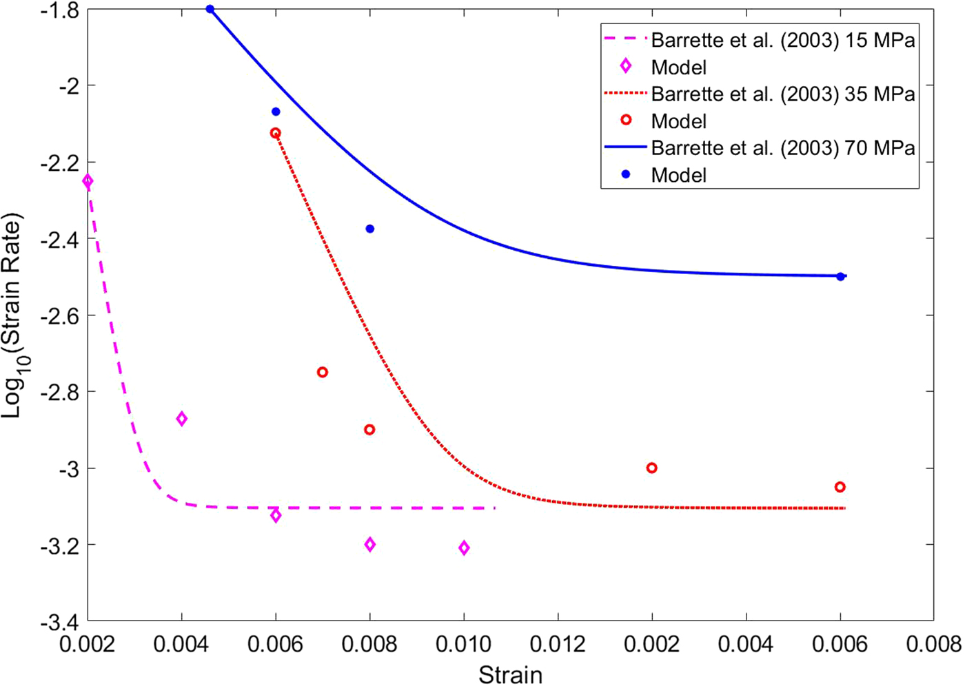
Fig. 8. Strain rate vs. axial strain at different confining pressures, computed with model (8) and the coefficients of Table 3b. Experimental data (small circles) of Barrette and Jordaan (Reference Barrette and Jordaan2003).
We finally remark that assumption b 2 > 0 is always fulfilled with the data of Tables 1a, 2a and 3a.
5. RESULTS AND DISCUSSION
It is well known that ice under applied stress experiences creep deformation. Thus creep tests, performed at constant stress, are often used to determine the deformation of the ice and, consequently, its rheological parameters.
The experimental data reported by Barrette and Jordaan (Reference Barrette and Jordaan2003), Mctigue and others (Reference Mctigue, Passman and Jones1985) and Jones and Chew (Reference Jones and Chew1983) clearly highlight that hydrostatic pressure causes polycrystalline ice to modify its rheology. This type of behavior is comparable to that found in many other materials where the viscosity can vary by a factor of as much as 1010% (Prusa and others (Reference Prusa, Srinivasan and Rajagopal2012); Bair (Reference Bair2015)). Experimental data concerning glaciers and rock glaciers show appreciable variation of the viscosity with the depth, as shown in Figure 2 of Kannan and Rajagopal (Reference Kannan and Rajagopal2013).
Tests performed on polycrystalline ice at constant temperature show that ice exhibits characteristics which cannot be adequately described by the classical Newtonian model. Indeed, the ice flow is often represented by a power-law constitutive model (Glen's law) that provides good estimates of shear stresses and overall kinematics in simple flow configurations. However, such a model excludes any normal stress effect, which is of great significance in ice mechanics. For this reason, here we consider a second-order fluid model that provides excellent agreement with primary and secondary creep. In particular, we generalize the model of Mctigue and others (Reference Mctigue, Passman and Jones1985) and that of Man and Sun (Reference Man and Sun1987), by proposing the constitutive Eqns (6) and (8), whose rheological parameters depend on the pressure p. Model (8) accounts for both shear thinning (as for Glen's law) and normal stress differences.
To assess the suitability of the proposed model, we determine the rheological coefficients using the experimental data referring to primary and secondary creep presented by Jones and Chew (Reference Jones and Chew1983), Mctigue and others (Reference Mctigue, Passman and Jones1985) and Barrette and Jordaan (Reference Barrette and Jordaan2003). The agreement is satisfactory, showing that both models are well suited for capturing the behavior of the strain curves as the pressure increases as proposed by Mctigue and others (Reference Mctigue, Passman and Jones1985), the two strain rate vs. strain curves of Fig. 1 in Jones and Chew (Reference Jones and Chew1983) and the three strain rates vs. strain curves of Fig. 3 in Barrette and Jordaan (Reference Barrette and Jordaan2003). One of the quintessential feature of this paper is to show that rheological models with pressure-dependent parameters are able to capture the ice creep enhancing due to high pressure. Actually, Kannan and Rajagopal (Reference Kannan and Rajagopal2013), using a constitutive model that takes into account the effect of the shear rate, pressure and the volume fraction of the rocks and sand grains trapped within the interstices are also able to reproduce quite satisfactorily the peculiar flow data of the Murt él-Corvatsch glacier.
Concerning the pressure dependence of the rheological parameters of models (6) and (8), we assumed a Barus-type law (9), (10).
Models (6) and (8) are still tentative. Theoretical and experimental work remains to be done in order to discern which of the two models is more appropriate for the creep flow of ice. Indeed, our analysis refers essentially to 1-D axial tests and not to shear tests. The latter could help in the selection of the constitutive model but could also bring out other phenomena such as a pressure-dependent shear thinning effects. Finally, it is well known that temperature greatly influences the flow properties of ice. By taking into account the effects of temperature one may be able to capture the motion more accurately.
Acknowledgments
We thank Dr. Ralf Greve, Hokkaido University, for his precious comments and useful suggestions that helped us improve this paper. We express our sincere gratitude to Prof. Raymond Ogden, University of Glasgow, and to Prof. Michel Destrade, NUI Galway, for their various comments on this work. We also thank the referees for their useful suggestions.


 Open access