


1. Introduction
Mass loss at the surface of a glacier is governed by the surface energy balance between the atmosphere and the glacier (Cuffey and Paterson, Reference Cuffey and Paterson2010). Turbulent fluxes are often considered secondary to radiative fluxes in glacier environments, but they can dominate the energy exchange under some conditions (Hock, Reference Hock2005). Turbulent heat fluxes are expected to be of increasing importance in a warming world (Intergovernmental Panel on Climate Change, 2014) and have been implicated in extreme melt events (e.g. Hay and Fitzharris, Reference Hay and Fitzharris1988; Fausto and others, Reference Fausto, van As, Box, Colgan and Langen2016; Thibert and others, Reference Thibert, Dkengne Sielenou, Vionnet, Eckert and Vincent2018). The inclusion of turbulent energy fluxes in glacier surface energy-balance models usually relies on bulk approaches that derive exchange coefficients for potential temperature and specific humidity in the boundary layer (e.g. Braithwaite and others, Reference Braithwaite, Konzelmann, Marty and Olesen1998; MacDougall and Flowers, Reference MacDougall and Flowers2011; Nicholson and others, Reference Nicholson, Prinz, Mölg and Kaser2013). The theory underpinning such approaches was developed for neutrally stratified, horizontally homogeneous flat terrain with constant fluxes with height (Lettau, Reference Lettau1934; Prandtl, Reference Prandtl and Durand1934), while the cold, sloping surfaces of mountain glaciers within steep mountain topography do not conform to these conditions (Denby and Greuell, Reference Denby and Greuell2000; Radic and others, Reference Radic2017). Snow or ice at the glacier surface is by definition consistently at the saturation point, and cannot reach temperatures above 0°C. The latter causes persistently stable conditions in the near surface boundary layer that require correction to standard bulk methods (e.g. Klok and others, Reference Klok, Nolan and van den Broeke2005; Conway and Cullen, Reference Conway and Cullen2013). Such a stable atmosphere causes the development of persistent katabatic winds, flowing down the sloping glacier surface, characterized by a low level jet. As a result, the glacier microclimate and surface melt regime is determined by such katabatic wind systems and their interaction with the wider valley circulation (van den Broeke, Reference van den Broeke1997; Oerlemans and Grisogono, Reference Oerlemans and Grisogono2002). Turbulent exchange at the glacier surface is strongly influenced by the katabatic flow, with its atypical vertical structure of the boundary layer (e.g. Smeets and others, Reference Smeets, Duynkerke and Vugts1998; Smeets and others, Reference Smeets, Duynkerke and Vugts2000). This atypical structure stems from the fact that the katabatic jet maximum height over mid-latitude glaciers is often at heights smaller than the surface Obukhov length thus invalidating Monin–Obukhov similarity theory (Parmhed and others, Reference Parmhed, Oerlemans and Grisogono2004; Grisogono and others, Reference Grisogono, Kraljević and Jeričević2007). With a jet maximum height below 10 m above the surface, a surface layer (lowest 10% of the boundary layer in which fluxes are constant with height, cf. Stull, Reference Stull1988) in katabatic flows is not expected to exceed the first meter above the surface and thus tends to be too shallow to be measured with standard turbulence instrumentation. Furthermore, turbulent exchange is also conditioned by surface roughness that, over glaciers, changes dramatically in space and time due to changing snow cover extent, and the formation of ablation topography and crevasses (Smeets and others, Reference Smeets, Duynkerke and Vugts1999; Brock and others, Reference Brock, Willis and Sharp2006).
The absence of a clearly observable surface layer, along with horizontal heterogeneity of the surface and the complex atmospheric circulation associated with a mountain glacier strongly influence the spatial patterns of surface exchange (Sauter and Galos, Reference Sauter and Peter Galos2016). As a result, direct measurements of turbulent fluxes over glacier surfaces show that standard theory of bulk turbulent exchanges perform poorly over glacier surfaces (Radic and others, Reference Radic2017). Finally, the effects of low frequency oscillations or coherent turbulent structures associated with katabatic winds or mesoscale flows respectively, are not captured in turbulent fluxes over glaciers calculated using bulk methods (e.g. Smeets and others, Reference Smeets, Duynkerke and Vugts1998; Litt and others, Reference Litt, Sicart, Helgason and Wagnon2014).
This poor performance of traditionally-used methods of calculating turbulent fluxes is of increasing concern given that the relative importance of turbulent fluxes to glacier ablation is expected to increase with projected climate warming of glaciated regions. Thus, it is vital to improve current understanding of the turbulent exchanges between glaciers and the atmosphere in order to understand how the changing climate influences glaciers, as well as how changing glacier surfaces might influence future atmospheric states and microclimates. However, the present paucity of suitable data over glacier surfaces limits deeper investigation of the processes of turbulence at the glacier–atmosphere boundary (Radic and others, Reference Radic2017).
Continued climate driven recession of mountain glaciers is expected to result in an increasing proportion of surface debris cover on remaining glaciers (Scherler et al., Reference Scherler, Wulf and Gorelick2018), and debris cover is a prominent feature of the regional scale ablation zone and glacier response in some mountain ranges (e.g. Scherler et al., Reference Scherler, Bookhagen and Strecker2011). Supraglacial rock debris cover has markedly different optical, thermal, moisture and roughness properties to snow or ice, and can thus be expected to alter the boundary conditions for turbulence production and energy exchanges at the glacier surface.
The sensitivity of the boundary layer structure to surface characteristics is readily seen through stability conditions. In contrast to the strong stability experienced over exposed glacier surfaces, above debris-covered ice, heating of the surface during sunny days causes strong convective instability transferring heat from the debris to the atmosphere, which is only weakened by strong wind conditions, or radiative cooling of the surface as the day ends (e.g. Mihalcea and others, Reference Mihalcea2006; Brock and others, Reference Brock2010; Shaw and others, Reference Shaw2016). The diurnal surface heating and thermal instability causes strong diurnal cycles in turbulent sensible heat exchange over debris-covered ice, with neutral stability conditions only briefly observed in the evening transition (e.g. Brock and others, Reference Brock2010).
A limited number of measurements of turbulent exchange over debris-covered ice (Collier and others, Reference Collier2014; Yao and others, Reference Yao, Gu, Han, Wang and Liu2014; Steiner and others, Reference Steiner2018) indicate that these fluxes play a non-negligible role in the surface energy balance of debris-covered glaciers, and moisture fluxes through processes of ventilation of the debris cover also provide an explanation of the characteristic shape of the Østrem curve of ice ablation as a function of debris thickness (Evatt and others, Reference Evatt2015). Treatment of debris-covered ice in coupled glacier land surface–atmosphere models shows that the altered surface properties of the debris-covered parts of the glacier impact the overlying atmosphere at a regional scale (Collier and others, Reference Collier2015), and such feedbacks may become more important to mountain weather as debris-covered ice areas expand to affect a greater proportion of the glacierized area. As is the case for exposed glacier ice, bulk approaches of treating turbulent exchange perform poorly over debris-covered ice (Steiner and others, Reference Steiner2018), and progress in exploring the impact of debris cover on glacier–atmosphere turbulent exchanges is hampered by a lack of primary observations over debris-covered glacier ice. Aerodynamic and geometric methods of determining roughness lengths for debris-covered glacier surfaces (e.g. Brock and others, Reference Brock2010; Miles and others, Reference Miles, Steiner and Brun2017; Quincey and others, Reference Quincey2017) show roughness varying widely with surface grain size as well as wind direction, but very few direct measurements of turbulent exchanges exist.
In this paper, we examine the properties of midsummer turbulence measured simultaneously over clean and debris-covered ice on a glacier in the European Alps to provide the first explicit comparison of how the near-surface turbulence and turbulent energy fluxes observed over these two glacier surface types compare. We investigate the nature of the turbulence and turbulent fluxes under different wind regimes, in the context of the glacier katabatic wind system, with the overall goal of providing valuable information for improving representations of turbulent fluxes over complex glacier surfaces.
2. Study area and field measurements
Suldenferner/Ghiacciaio de Solda is the name given to a number of glacier bodies in the Italian Alps that have separated during their retreat since the Little Ice Age glacier advance. The westernmost glacier body, which is the focus of this study, descends from Ortler/Ortles (3905 m) and is largely debris-covered below 2900 m. This debris-covered glacier is ~3 km long, and 0.5–0.9 km wide, spanning the elevation range of ~3350–2600 m.
Given the logistical challenges of transporting and installing meteorological towers on relatively inaccessible glacier surfaces, it is appealing to use light, minimal station installations. Here we use two single-height eddy covariance (EC) systems and a longer-serving automatic weather station (AWS) to collect near-surface meteorological observations at locations on the glacier surface with contrasting surface properties (Fig. 1). The upper EC station (ecci) was installed in clean ice (46.498° N/10.560° E) at an elevation of ~2780 m, and the lower EC station (ecdc) was located in debris-covered ice (46.495° N/10.572° E) at ~2600 m, where local debris thickness was ~0.08 m, though excavations at 100 m intervals across the whole debris-covered area indicate that mean debris thickness is 0.14 m (interquartile range of 0.06–0.16 m). Multiple field sightings at the time of installation indicated surface slope at both EC sites to be between 2° and 5°, although a steeper slope section separates ecci and the AWS.
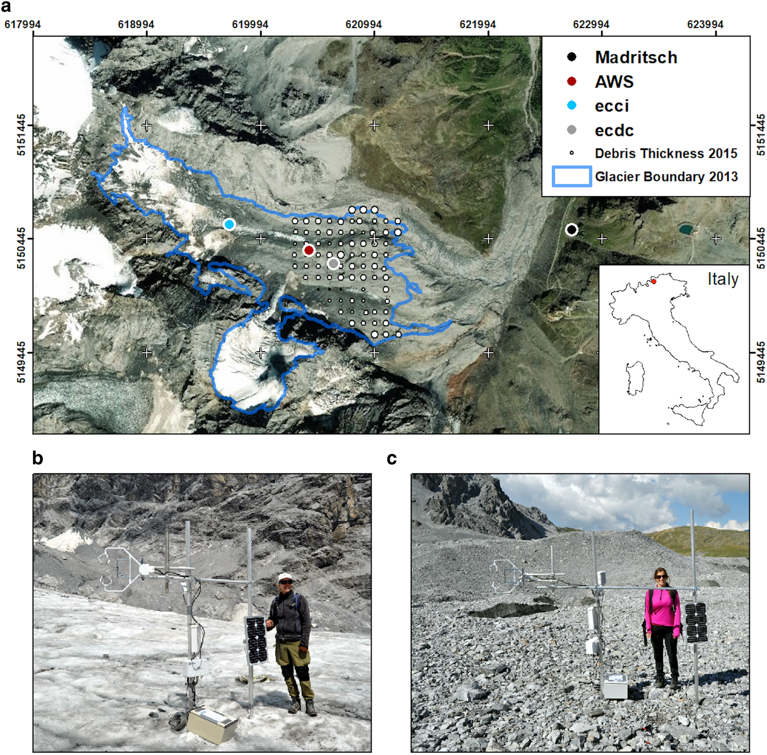
Fig. 1. (a) Map of Suldenferner in UTM (32N) coordinates showing the location of all meteorological stations used in this study. The glacier outline is from 2013 (from Galos and others, Reference Galos2015); debris extent is shown in the ESRI basemap imagery from 2017; point measurements of debris thickness measured by excavation in summer 2015 are shown in scaled circles, from 0.01 to 0.6 m debris thickness. The EC installations over clean (ecci) and debris-covered (ecdc) ice are shown in (b) and (c), respectively.
The AWS is located between the two EC installations, below the upper boundary of the continuous debris cover (46.496° N/10.569° E) at ~2625 m, where local debris thickness was ~0.09 m. The AWS consists of a Kipp and Zonen CNR1 4-way radiation sensor, a shielded Vaisala HMP45c temperature and relative humidity sensor, and a Young 05103 anemometer. The 30-min averages and sds of variables were recorded by using a Campbell C3000 data logger. Temperature and relative humidity are also sampled at 30-min intervals allowing the vapor pressure to be calculated at this interval. All station locations were recorded using a hand-held Garmin GPS, with an accuracy of ±5–8 m.
The EC instrumentation was identical at both stations and consisted of two segmented masts drilled into the ice with sensors mounted at a height of 1.6 m on a cross arm spanning the vertical masts (Figs 1b, c). A CSAT 3D sonic anemometer and KH20 hygrometer sampling data at a frequency of 20 Hz were mounted parallel to the surface and facing obliquely across-glacier at a bearing of 255° so as to capture both up- and down-glacier winds. In choosing the height of the single-level EC instrumentation, we ideally wish to sample below any potential glacier katabatic jet maximum height, which over the sloping surface of a small glacier like Suldenferner can be below 2 m (Denby and Greuell, Reference Denby and Greuell2000; Oerlemans and Grisogono, Reference Oerlemans and Grisogono2002). However, the instruments cannot be installed too close to the surface because with a transducer spacing of 10 cm, installation very close to the surface will result in detrimental high frequency signal losses (Aubinet and others, Reference Aubinet, Vesala and Papale2012), and also reduce the sampled footprint size, which may affect the representativeness of the measurements. A shielded Vaisala HMP45 was installed on the EC mast to record 1-min averages of air temperature, relative humidity and vapor pressure. Data were recorded using Campbell Scientific CR1000 data loggers with compact flash card storage modules. Power was provided by 60 Ah deep cycle batteries connected to 20 W solar panels.
The EC station over debris-covered ice was installed on 10 August 2015, and the one over clean ice was installed on 11 August 2015. Although we intended to collect 7–10 days of continuous data, a number of instrumental failures prevented that. At ecdc, a faulty solar panel regulator resulted in this station losing power at the end of 14 August. At ecci, two instrument failures occurred; the Vaisala instrument on the afternoon of 12 August and the KH20 at the end of 14 August. Conditions were not exceptionally harsh and no meaningful explanation of these failures could be identified. As a result, we focus on the short common period of EC data spanning 13.45 UTC (14:45 local time) on 11 August to 21.00 UTC on 14 August.
The EC method and high frequency data were used to calculate kinematic fluxes at both EC stations. In the absence of pressure data at any of the on-glacier stations, elevation-corrected air pressure from a nearby mountain weather station was used to convert the kinematic fluxes to energy fluxes to facilitate comparison with other studies. Madritsch weather station (46.494° N/10.614° E), operated by the Autonomous Province of Bozen lies 3.4 km to the east at an elevation of 2825 m (Fig. 1), and provided the required variables stored as 10-min averages (http://wetter.provinz.bz.it/; station ID: 115). As we are also missing low frequency temperature and humidity data at ecci for part of the study period we also need to reconstruct these data from other observations. This was done using a multilinear regression analysis (e.g. Wilks, Reference Wilks2011) to establish a relationship between the high frequency and low frequency measurements at the ecci site for the available period of overlapping data. The data processing and corrections are described in the following section.
3. Data processing and analysis
EC data were processed assuming no zero plane displacement and in line with the convention usual for cryospheric sciences, sensible and latent heat fluxes are expressed as positive if the direction of the flux is toward the surface. This is opposite to the convention applied to turbulence studies in atmospheric sciences.
The averaging interval for the computation of turbulence statistics was chosen on the basis of multi-resolution flux decomposition (MRD; Howell and Mahrt, Reference Howell and Mahrt1997; Vickers and Mahrt, Reference Vickers and Mahrt2003), which decomposes the data variability into different scales to determine how each time interval contributes to the turbulent flux.
MRD can also be used to reveal any differences in scale-wise structure of turbulence over different surfaces or under different stability conditions. The timescale at which the MRD of the sensible heat flux (Cwθ) approaches zero indicates the transition between turbulent and mesoscale processes. The results indicate that the majority of the turbulent flux variability is captured by a 5 min averaging interval over both surfaces and under both stable and unstable conditions (Fig. 2), while excluding mesoscale processes, so this period was chosen for block averaging for subsequent analysis.

Fig. 2. Example of MRD shown for heat flux for all the periods when the heat flux over debris-covered ice (ecdc) was (a) negative, indicating unstable near surface temperature profile and (b) positive, indicating stable near surface temperature profile. Data presented are bin averages with shading showing the inter-quartile range. The timescale at which the flux contributions transition from turbulent scale to mesoscale is indicated by the curves approaching zero.
Double coordinate rotation and linear detrending were applied over each averaging block prior to deriving turbulent statistics (e.g. Stiperski and Rotach, Reference Stiperski and Rotach2016). Double rotation in effect corrects for any misalignments of the instruments with respect to the mean surface slope and wind direction, by rotating the coordinate system such that vertical and lateral wind vectors equal zero over the chosen averaging interval. Subsequent analysis thus represents surface normal fluxes (expressed by the w coordinate) with respect to the surface parallel (streamwise) wind direction (expressed as the u coordinate). Linear detrending of each averaging period was used to remove the possible remaining trends due to contribution of the non-turbulent larger-scale motions such as mesoscale processes or diurnal cycle over the averaging period to the turbulent fluxes. Finally, fluxes were corrected for path averaging of the sensor (Moore, Reference Moore1986), sensible heat flux was additionally corrected for humidity effects (Schotanus and others, Reference Schotanus, Nieuwstadt and de Bruin1983), and latent heat flux was corrected for oxygen effects (van Dijk and others, Reference van Dijk, Kohsiek and de Bruin2003) and density effects (Webb and others, Reference Webb, Pearman and Leuning1980).
For averaging periods in which the stability (z/L) was near-neutral, that is within |0.05 | of zero (Sfyri and others, Reference Sfyri2018), surface roughness length for momentum was calculated from the logarithmic wind profile for each station:

where z is the measurement height, $\bar{U}$ is the wind speed and friction velocity is calculated as $u^\ast{=} \;\lpar {{\overline {u{\rm^{\prime}}w{\rm^{\prime}}} }^2 + {\overline {v{\rm^{\prime}}w{\rm^{\prime}}} }^2} \rpar ^{1/4}$
 . The near-neutral conditions were satisfied in 130 5-min periods at ecci and 141 at ecdc. We considered this sample of near-neutral data sufficient for the analysis and so have not used periods where a stability correction would be necessary as, due to the existence of a low level jet maximum at heights smaller than the surface Obukhov length, it is questionable if such a stability correction is even appropriate (cf. Nadeau and others, Reference Nadeau, Pardyjak, Higgins and Parlange2013).
Information on anisotropy of turbulence allows quantification of the degree to which the turbulence is deformed by the closeness to the surface, wind shear or buoyancy, and can also offer further information on the mechanism by which turbulence is produced. Turbulence anisotropy was calculated from the full, un-corrected, Reynolds stress tensor following Stiperski and Calaf (Reference Stiperski and Calaf2018). Since only the anisotropic part of the Reynolds stress tensor can transport momentum (Pope, Reference Pope2000), we first subtract the isotropic contribution to the Reynolds stress tensor and normalize it by TKE to define the non-dimensional anisotropy stress tensor with components:

Here, $\overline {u_iu_j}$ are the components of the Reynolds stress tensor and δ ij is the Kronecker delta.
The three eigenvalues of this symmetric tensor can be used to finally define a set of two independent scalar invariants that describe the state of anisotropy (Lumley and Newman, Reference Lumley and Newman1977). The state of anisotropy can therefore be uniquely represented in the anisotropy invariant map (e.g. Pope, Reference Pope2000). Here we use the invariants defined in the barycentric Lumley triangle representation of the anisotropy invariant map (Banerjee and others, Reference Banerjee, Krahl, Durst and Zenger2007):


where λ 1, λ 2 and λ 3 are the three eigenvalues of tensor defined in non-dimensional anisotropy stress tensor. Given the triangular nature of the anisotropy invariant map we can identify three limiting states of anisotropy: isotropic, two-component axisymmetric and one-component topologies. Information on anisotropy of turbulence therefore allows quantification of the degree to which turbulence is deformed by the closeness to the surface, wind shear or buoyancy, and can therefore offer information on the mechanism by which turbulence is produced (Stiperski and Calaf, Reference Stiperski and Calaf2018).
To fill in the gaps in the low frequency data needed for converting kinematic fluxes into dynamic fluxes, the following procedures were applied. Pressure at the glacier stations (p) was calculated from the Madritsch weather station air pressure (p M at observation height h M) to the on-glacier station heights (h) and using the temperature at Madritsch (T M) and at AWS (T) as the mean temperature of the layer:

Here, the Madritsch data were linearly interpolated to 5 min to match the EC data. The time-averaged mean ecci air temperature (T ecci) was reconstructed by applying multi-linear regression using the sonic temperature (T sonic), and kinematic sensible $\lpar \overline {w{\rm ^{\prime}}\theta {\rm ^{\prime}}} \rpar$ and latent $\lpar \overline {w{\rm ^{\prime}}q{\rm ^{\prime}}} \rpar$
 heat fluxes as predictors:

during the 1-day period when all sensors at ecci were operating.
The results (Fig. 3) indicate that a robust relationship could be found in this way (R 2 value was 0.8 at a significance level p < 0.001), with the lower night-time temperatures slightly better captured than daytime. The median difference between the reconstructed and observed temperature is below the instrument precision at −0.06°C. To further evaluate this reconstructed record and fill in the intermittent gaps we applied the same process at the debris-covered ice, where comparison to the measurements throughout the period shows an even higher correlation (R 2 value was 0.98 at a significance level p < 0.001). The reason for this could be a more representative sample for regression. Missing low frequency vapor pressure at ecci was reconstructed from the product of mean absolute humidity from the KH20 (a KH20) and the mean sonic temperature (cf. ideal gas law) using linear regression (R 2 values was 0.99 at p < 0.001):

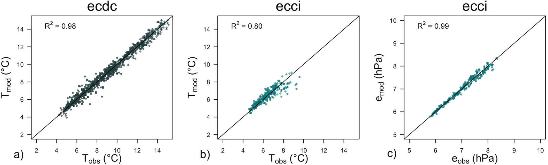
Fig. 3. Comparison of measured temperatures at ecdc (a) and ecci (b), and measured vapor fluxes at ecci (c) with those reconstructed using the transfer functions.
The vapor pressure reconstruction was applied as long as the KH20 instrument was functioning, so the reconstructed data series ends during 14 August.
Climatological flux footprints were calculated for each station and for each study period, using the footprint model of Kljun and others (Reference Kljun, Calanca, Rotach and Schmid2015). Although this model is not specifically designed for use in sloping terrain it can serve as a first guess for the flux source area for lack of better alternative. Given the large uncertainty in the boundary layer height and the wide range of glacier surface roughness lengths available in the literature (Brock and others, Reference Brock, Willis and Sharp2006; Miles and others, Reference Miles, Steiner and Brun2017) we have estimated the maximum and minimum footprints for each site. For the maximum footprint we used the boundary layer height of 10 m together with a minimum roughness from the literature for clean ice (z 0 = 0.005 m) and debris cover (z 0 = 0.016 m), while for the minimum footprint we used the boundary layer height of 100 m, with maximum roughness over clean ice (0.08 m) and debris cover (0.1 m).
Due to the low and varying height of the glacier katabatic jet, single-height sensors cannot consistently measure the properties at a fixed location within the katabatic wind profile, which requires further consideration as the jet maximum height exerts a strong control on turbulence profiles of streamwise fluxes (e.g. Denby and Smeets, Reference Denby and Smeets2000; Grachev and others, Reference Grachev2016). Grachev and others (Reference Grachev2016) show that below the jet maximum the streamwise momentum flux $\lpar \overline {u{\rm ^{\prime}}w{\rm ^{\prime}}} \rpar$ is negative, consistent with positive shear, the sensible heat flux (H) is positive consistent with the warmer air being transported downward by turbulence, and the streamwise heat flux $\lpar \overline {u{\rm ^{\prime}}\theta {\rm ^{\prime}}} \rpar$
 is also positive. The magnitude of the fluxes and TKE is largest at the surface and decreases toward the jet maximum height. At the jet maximum TKE has a minimum, while $\overline {u{\rm ^{\prime}}w{\rm ^{\prime}}}$
 and $\overline {u{\rm ^{\prime}}\theta {\rm ^{\prime}}}$
 both change sign so that above the jet maximum $\overline {u{\rm ^{\prime}}w{\rm ^{\prime}}} \;$
 becomes positive due to negative vertical wind shear, and $\overline {u{\rm ^{\prime}}\theta {\rm ^{\prime}}}$
 becomes negative. On the other hand, the sensible heat flux does not exhibit the same sensitivity to the jet maximum height but is either shown to vary semi-linearly across the jet maximum (Denby, Reference Denby1999; Grisogono and Oerlemans, Reference Grisogono and Oerlemans2001; Axelsen and van Dop, Reference Axelsen and van Dop2009) or is semi-constant (cf. Grachev and others, Reference Grachev2016; Stiperski and others, Reference Stiperski, Whiteman, Holtslag, Lehner and Hoch2019b). These findings have several major consequences relevant to our study. The first is that measurements in the presence of a low-level jet are not representative of the canonical surface layer and therefore also not of the surface fluxes. The second is that based on the sign of the streamwise fluxes we can determine if our single-height measurements were taken above or below the jet maximum. The third is that despite this large sensitivity of streamwise turbulence fluxes to jet maximum height, if the jet maximum heights at the two stations are close to each other, the sensible heat flux measurements can still be compared between the stations.
4. Results and discussion
4.1 General observations
The measurement period was chosen to coincide with a fair weather window at Suldenferner, to avoid snowfall and storm conditions that can occur throughout the summer at this site. Accordingly, meteorological conditions during the measurement period in August 2015 were warm, mostly sunny, with some cloudy spells, and characterized by strong diurnal cycles in net radiation, temperature and relative humidity. Wind speed variability was not related to the diurnal cycle, and average wind speed was 2.9 m s−1 and did not fall below 1.0 m s−1 (Fig. 4). For the portion of the study period for which temperature and relative humidity data were recorded at all three stations, air temperature was never below 5°C and, while nocturnal air temperature and relative humidity are comparable at all three stations, the two debris-covered locations show mid-day temperatures 5–7°C warmer, and relative humidity 15–25% lower, than recorded above the exposed ice. On the basis of surface lowering measured at ablation stakes drilled into the glacier ice and measured over a 10-day period spanning the period of common data, surface lowering over the course of our analysis was estimated to be 0.11 m at the clean ice site and 0.07 m at the debris-covered site.

Fig. 4. Time series of net radiation (R n), air temperature $\lpar \bar{T}\rpar$ and relative humidity (RH) recorded at the AWS, alongside 5 min (thin line) and 30 min averaged (thick line) fluxes of sensible heat (H), latent heat (LE), wind speed $\lpar \bar{U}\rpar$
 and direction (dir) measured at the AWS, the clean ice EC site (ecci) and the debris-covered EC site (ecdc). Shaded areas correspond to sub-periods classified as nighttime (light blue), daytime (yellow) and disturbed 1 (dark pink) disturbed 2 (light pink), described in Section 4.2.
Despite instrument testing and fairly clement conditions on the glacier, two instrument failures occurred, which highlights the advantage of either transmitting data to a base location for regular review, or remaining in attendance even for short field campaigns. Nevertheless, given the paucity of direct turbulence measurements from glaciers, and particularly debris-covered glaciers, the findings from even this short investigation period have value, and allow us to make a number of observations about the turbulence processes operating in different wind regimes at this glacier.
4.2 Observed wind regimes and sampled footprint
The wind regimes during the study period can be seen in Figures 4 and 5. We use the wind conditions, in conjunction with the calculated heat fluxes, to subset the data into contrasting regimes for subsequent analysis: nocturnal katabatic conditions, clear sky daytime conditions and two periods of disturbed wind conditions with contrasting sky conditions and fluxes (Fig. 4).

Fig. 5. Flux footprints for the four examined periods, for the ecci and ecdc stations overlain on DigitalGlobe imagery of 2019. The footprints are climatological and were calculated for all 5 min fluxes that fall within the examined periods. The larger footprint was calculated with boundary layer height equal to 10 m and the lower limit of the literature surface roughness for clean ice and debris-covered ice. The smaller footprint was calculated for boundary layer height equal to 100 m and the upper limit of the literature surface roughness for clean and debris-covered ice.
Wind direction in the first half of the common data period was predominantly down-glacier at all measurement sites, indicative of a prevailing glacier katabatic wind system, even though this glacier is relatively small. During the night down-glacier flow was persistent and wind speed, temperature and relative humidity were relatively constant at all sites, indicating the penetration of the katabatic flow over the debris-covered part of the glacier (Fig. 4). Based on the consistent wind directions at all sites, we select the night time periods at the end of 11 and 12 August as examples of stable nocturnal conditions (labeled ‘night’ in figures), experiencing downslope flow at all sites, allowing us to examine turbulence at the two sites under comparable wind conditions.
During sunny daytime conditions the lowest debris-covered site experiences episodic up-glacier flow and the AWS location experiences a mixture of airflow from up-glacier, from the tributary glacier to the south, and occasionally from down-glacier. During these sunny days, wind speed decreases down-glacier, and the varying wind direction over the debris cover is indicative of episodic penetration of the katabatic wind interspersed with more upvalley flow, also reflected in the presence of a consistent down-glacier-increasing temperature and down-glacier-decreasing relative humidity gradient across the sites. Based on the incoming shortwave radiation, 12 August is selected to represent clear sky sunny conditions (labeled ‘day’ in figures), as 13 August shows more mixed conditions, starting sunny but clouding over in the afternoon (Fig. 4). This data subset samples a period when wind and thermal properties differ the most between the two EC measurement sites.
While the exposed ice site experiences consistent down-glacier wind during 12 and most of 13 August, during the daytime of 14 August the wind regime changed dramatically, illustrating a case when the glacier katabatic wind regime is disturbed by larger-scale flow bringing cooler, cloudier conditions in the following days. During the disturbed wind regime of 14 August there is a dramatic switch to up-glacier airflow at all sites, with lower wind speed and more variable flow direction over the exposed ice site (Fig. 4). This variable flow direction at ecci probably indicates interplay between nascent katabatic flow over the exposed part of the glacier and the disturbance of the up-glacier airflow. This disturbed airflow encompasses a period of clear sky conditions (labeled ‘disturbed 1’ in figures) followed by cloudy conditions in the second part of the day (labeled ‘disturbed 2’ in figures). These periods of disturbed airflow allow us to compare conditions at the two turbulence sites under the influence of a wind regime not stemming from the glacier-driven circulation.
The differences in wind regimes are also reflected in the flux footprints (Fig. 5). The footprints are presented in terms of contours that encompass 80% of the flux source area for combinations of boundary layer depth and surface roughness from the literature over clean and debris-covered ice that generate maximum and minimum footprints. Given that the footprint models were not developed for use in complex terrain, the calculated footprints should be considered indicative only. Still, they show that the measurements are expected to sample appropriate surfaces for comparison of clean and debris-covered ice processes. The potential flux source area for the clean ice station is persistently over clean ice but during the disturbed period could extend down to the beginning of the debris cover at its largest extent (Fig. 5d). The footprints for the debris-covered station are also consistently over debris cover, but show more variable wind direction and larger footprint areas during the daytime and under disturbed conditions compared to the exposed ice site.
4.3 Turbulent properties: stability, z 0, TKE and anisotropy
The dimensionless stability parameter (z/L where L is the Obukhov length) shows persistently stable conditions over the exposed ice as expected under these midsummer conditions (Fig. 6), with mean conditions during clear-sky daytime being slightly more stable (Fig. 7). Over the debris-covered ice, stable nocturnal profiles rapidly become unstable once the glacier surface is in the sunlight (Fig. 6). Importantly, the disturbed airflow under cloudy conditions brings both surface types closer to neutral stability even during the daytime (Fig. 7). This shows that strong synoptically- or valley-driven winds are able to reduce the intensity of the near-surface stability over the glacier and also indicates that time-variant stability conditions should be considered even over exposed ice surfaces. In addition, the reduced stability might be partially related to the flux footprint of the clean ice station extending toward the debris cover (Fig. 5) and potentially advecting heat up-glacier toward the exposed ice, during which the streamwise heat flux over the exposed ice indicates a positive tendency.

Fig. 6. Time series of 5 min (thin line) and 30 min averaged (thick line) dimensionless stability parameter (z/L), turbulent kinetic energy production (TKE) and friction velocity (u*). Colors as in Figure 4.

Fig. 7. Median (black line), interquartile range (boxes) and outlier (whiskers) values of wind speed $\lpar \bar{U}\rpar$ , turbulent kinetic energy production (TKE), sensible heat flux (H), temperature variance $\lpar \overline {\theta ^2} \rpar$
 and stability (z/L) for clean ice (ecci) and debris-covered ice (ecdc) stations for all of the data and the four periods identified in Figure 4.
Although it might be intuitive to expect the debris-covered ice, supporting rocks and boulders up to sizes >1 m, to have a larger roughness than the exposed ice surface, the calculated surface roughness lengths are similar at both measurement sites on this glacier (Fig. 8). It is worth noting that the surface undulations of the debris-covered glacier portion at Suldenferner are much less pronounced than within the hummocky terrain characteristic of debris-covered glaciers in, for example, the Himalaya (e.g. Miles and others, Reference Miles, Steiner and Brun2017), which might be expected to exert an additional surface roughness component at the decimeter scale.

Fig. 8. Surface roughness length for momentum (z 0) over exposed ice (ecci) and debris-covered ice (ecdc), (a) plotted as a function of wind speed and (b) direction for cases where wind speed is >3 m s−1.
The surface roughness length at both sites is strongly dependent on wind speed with large outliers occurring at low wind speeds (Fig. 8). Following Radic and others (Reference Radic2017), Fitzpatrick and others (Reference Fitzpatrick, Radić and Menounos2017) and Fitzpatrick and others (Reference Fitzpatrick, Radić and Menounos2019) we filter our roughness estimates for wind speeds in excess of 3 m s−1. This filter leaves 15 and 65 instances of calculated roughness for wind speeds >3 m s−1 at ecci and ecdc, respectively, and these give median (maximum) roughness lengths of 0.037 (0.140) m and 0.015 (0.069) m at these sites, respectively. These upper bound values are comparable to the maximum values estimated for complex bouldery terrain on debris-covered glaciers (cf. Miles and others, Reference Miles, Steiner and Brun2017). At higher wind speeds the values for two stations also show only marginal differences. During up-glacier airflow at ecci, roughness values do not show such a clustering at low values but are instead more spread. We speculate that this could be due to footprints of ecci station encompassing more crevassed areas down-glacier of the station (Fig. 5), but this cannot be verified from the available data.
The level of turbulence expressed by TKE is generally comparable during the night periods, and over much of the study period (Figs 6, 7), which is expected given the similarity of the surface roughness at the two measurement sites (Fig. 8). Over the exposed ice the difference in TKE between the night and day sample periods scales with wind speed. However, over the debris-covered ice, periods of instability during sunny conditions produce an additional buoyant component of TKE, causing TKE to be higher over the debris than exposed ice during clear sky conditions even though the corresponding wind speed is lower over debris cover than clean ice (Figs 6, 7).
During the disturbed airflow periods, when winds were coming from a more up-glacier direction (Fig. 4), the level of turbulence increases by up to a factor of 10 over both surfaces, despite the wind speed values being just above average velocities over the debris cover, and lower than average velocities over the exposed ice (Figs 6, 7), pointing to a change in the turbulence regime. Such a regime transition could indicate the establishment of a logarithmic-type wind profile. However, the comparatively large TKE values of up to 3 m2 s−2 might also indicate a downslope-windstorm type flow (cf. Haid and others, Reference Haid2019) where potentially other sources of TKE, such as TKE advection, might substantially contribute to the TKE budget. This change in turbulence regime is also evident in greater low frequency power in the spectra during disturbed flow, indicating the greater contribution of mesoscale activity to the turbulence (Vercauteren and others, Reference Vercauteren, Boyko, Kaiser and Belušić2019), and in the turbulence anisotropy (Fig. 9).

Fig. 9. Turbulence anisotropy for clean ice (ecci) and debris-covered ice (ecdc) stations for all of the data and the four periods identified in Figure 4, plotted within the barycentric anisotropy map where the axes show the anisotropy invariance as defined in Section 3 (cf. Stiperski and Calaf, Reference Stiperski and Calaf2018). The points represent 5-min periods, and colors the limiting states of anisotropy: green – isotropic, blue – two-component turbulence and red – one-component turbulence. The black square shows the center of mass of the points within the barycentric map.
The anisotropy of the Reynolds stress tensor partitioned into three limiting states of isotropic, two-component and highly anisotropic one-component (Fig. 9) reveals that, due to the instruments being close to the surface at both stations, turbulence is never isotropic. The turbulence over both the debris cover and clean ice shows very similar anisotropy: more isotropic during the katabatic and daytime periods, becoming more anisotropic during the disturbed periods when strong shear due to large wind speed further distorts turbulence. These results suggest that the same kind of similarity approach could be applied to both surfaces (Stiperski and others, Reference Stiperski, Calaf and Rotach2019a). The largest difference between the two surface types is, as expected, observed during the clear sky daytime conditions where turbulence is more anisotropic and closer to two-component over debris cover than over exposed ice.
4.4 Comparison of turbulent fluxes
Over exposed ice the sensible heat flux remains relatively constant under all conditions (Figs 4, 7), and is typically an energy source for the glacier surface, though brief negative flux periods do occur in all but the sunny daytime conditions (Fig. 4). Over the whole sampled period, positive sensible heat flux also predominates over the debris cover, but this changes abruptly to strongly negative heat fluxes during periods when the surface receives direct solar radiation (Figs 4, 6). During the disturbed periods, the positive sensible heat flux increases over the exposed ice pointing to increased mixing of warmer air toward the glacier ice. This could also indicate an advective heat contribution from the proximal debris cover (cf. Fig. 5) or larger-scale subsidence due to dynamically induced winds such as föhn (cf. Haid and others, Reference Haid2019). On glaciers with thicker debris (e.g. Miage Glacier, Italian Alps, 0.25 m; Lirung Glacier, Langtang Himalaya, 0.75 m and Koxkar Glacier, Tien Shan, China, 1.6 m) sensible heat fluxes were found to be generally negative, and reach daily maxima on the order of −50 and −200 W m−2 during midsummer or late monsoon (Collier and others, Reference Collier2014; Yao and others, Reference Yao, Gu, Han, Wang and Liu2014; Steiner and others, Reference Steiner2018). Values of negative heat fluxes comparable to those previously published are only observed during the sunny daytime conditions on Suldenferner. In contrast to previously published values for other glaciers with thicker debris cover, our data at ecdc show more predominantly positive heat fluxes prevail during the night and cloudy conditions, which may be favored by the thinner debris at Suldenferner.
Latent heat fluxes are an order of magnitude smaller than the sensible heat fluxes (Fig. 4), and are typically slightly positive over the exposed ice, and during the night are also positive to the debris-covered ice surface (Fig. 6). This is interesting as it implies that the tendency across the whole glacier is for moisture deposition onto the surface during these midsummer conditions, and moisture is only transferred to the atmosphere during the strong heating and convection phases under clear sky conditions over the debris-covered ice. This runs counter to previous studies that assume that the dryness of the debris surface implies negligible latent heat flux, and suggests that moisture is evacuated from and through the debris cover to the overlying air (cf. Evatt and others, Reference Evatt2015). It also reveals that at least small amounts of moisture are likely deposited onto the debris cover during the night. This is potentially significant as this moisture, along with moisture from precipitation events, can impact the bulk thermal properties of the layer (Nicholson and Benn, Reference Nicholson and Benn2012). Latent heat flux measured at other debris-covered glaciers shows a stronger and more consistent diurnal variability than is seen at Suldenferner, and typically remains negative during ablation season conditions (Collier and others, Reference Collier2014; Yao and others, Reference Yao, Gu, Han, Wang and Liu2014; Steiner and others, Reference Steiner2018). This again could potentially be a result of lower nocturnal surface temperatures over Suldenferner due to the thin debris cover.
4.3 Katabatic jet height and glacier scale influence
Examining the sign of the measured $\overline {u{\rm ^{\prime}}w{\rm ^{\prime}}}$ and $\overline {u{\rm ^{\prime}}\theta {\rm ^{\prime}}}$
 at Suldenferner in light of the expected structure in relation to a katabatic jet maximum (Fig. 10) we can conclude that over exposed ice our measurements at 1.6 m are approximately at, or above, the katabatic flow maximum, whereas over debris cover the katabatic depth is greater as the measurements at 1.6 m are below the katabatic jet maximum. This increase in the depth of katabatic flow could be due to a change in slope angle upstream of ecdc site (cf. Smith and Skyllingstad, Reference Smith and Skyllingstad2005). During the day, the depth of the katabatic jet increases over clean ice and the values of $\overline {u{\rm ^{\prime}}w{\rm ^{\prime}}}$
 and $\overline {u{\rm ^{\prime}}\theta {\rm ^{\prime}}}$
 become closer to zero as the jet maximum height approaches the measurement height of 1.6 m. Therefore, the small values of the streamwise fluxes and TKE at the clean ice site (Figs 6, 10) could be due to the jet maximum being very close to the measurement height.

Fig. 10. Median (black line), interquartile range (boxes) and outlier (whiskers) flux values of (a) sensible heat, (b) latent heat, (c) streamwise moisture and (d) streamwise heat normal for clean ice (ecci) and debris-covered ice (ecdc) stations for all of the data and the four periods identified in Figure 4.
The fact that our measurements appear to be close to and variably above and below the jet maximum height raises the question of the degree to which they are influenced by the surface, and whether it is fair to compare fluxes above and below the jet maximum. First, the fact that TKE is non-negligible in the measurements over clean ice, even though the measurements are apparently frequently above the jet maximum, suggests that the near-surface inversion is shallow and the air above the jet is less stable, allowing turbulence to develop anew. From this we can conclude that the measurements are not above the turbulent boundary layer. This is reinforced by the anisotropy analysis in which the lack of one-component anisotropy during katabatic periods confirms that turbulence measured above the jet is still well developed and within the turbulent boundary layer (cf. Stiperski and Calaf, Reference Stiperski and Calaf2018; Stiperski and others, Reference Stiperski, Calaf and Rotach2019a). Second, although the jet maximum height imposes a strong control on momentum fluxes, along-slope heat flux, TKE and temperature variance, the existence of a jet maximum has a lesser effect on sensible heat flux. Theoretical and modeling studies (Denby, Reference Denby1999; Grisogono and Oerlemans, Reference Grisogono and Oerlemans2001; Axelsen and van Dop, Reference Axelsen and van Dop2009) suggest that the sensible heat flux varies almost linearly across the jet maximum, while measurement studies (Grachev and others, Reference Grachev2016; Stiperski and others, Reference Stiperski, Whiteman, Holtslag, Lehner and Hoch2019b) suggest that above the jet maximum the sensible heat flux is almost constant.
Therefore, given that both of our stations measure very close to the jet maximum, the difference between the heat fluxes at the measurement height due to the exact position of the jet maximum can be assumed negligible. A comparison of the relationship between the sensible heat flux, mean wind speed and TKE for the ecci and ecdc stations during periods with katabatic flow (Fig. 11) shows little difference in the relationship between the variables at the two sites, despite differences in the depth of the katabatic flow. This is intuitive since the difference of surface roughness between the sites is not significant for cases with strong winds. Taken together, these lines of evidence suggest that comparing the fluxes at these two stations is justified. However, the heat fluxes measured at 1.6 m will necessarily present only a fraction of the true surface sensible heat flux due to significant decrease of heat flux with height below the jet maximum indicative of the non-existence of a surface layer in such shallow katabatic flows (cf. Stiperski and others, Reference Stiperski, Whiteman, Holtslag, Lehner and Hoch2019b).

Fig. 11. Sensible heat flux and linear regression relationship as a function of wind speed (ecci: R 2 = 0.38; 15.27 × U − 10.51; ecdc: R 2 = 0.18; 7.74 × U + 11.33), and TKE (ecci: R 2 = 0.25; 129.9 × TKE + 14.45; ecdc: R 2 = 0.36, 106.8 × TKE + 17.91), for katabatic periods over clean (ecci) and debris-covered ice (ecdc).
At Suldenferner, which is a small, partially debris-covered mountain glacier, prevailing katabatic winds appear to be readily disrupted by synoptic weather events. Furthermore, during sunny days it appears that convection over the sun-warmed debris cover prevents the katabatic wind system from penetrating to the glacier terminus. Instead the debris-covered zone of Suldenferner is characterized by gentler intermittent up-glacier airflow, and for large debris-covered Himalayan glaciers, valley scale circulation dominates over the lower, debris-covered portion of the glacier tongue (Steiner and others, Reference Steiner2018; Potter and others, Reference Potter, Orr, Willis, Bannister and Salerno2018).
The breakdown of katabatic winds over the debris-covered ablation zone has been previously noted (Brock and others, Reference Brock2010), and is analogous to the disruption of katabatic winds by advection of warm air from surrounding land surfaces at glacier margins (Jiskoot and Mueller, Reference Jiskoot and Mueller2012; Ayala and others, Reference Ayala, Pellicciotti and Shea2015). The wide variance of temperature lapse rates over some debris-covered glaciers (e.g. Mihalcea and others, Reference Mihalcea2006), may be at least partly due to this interplay between glacier and valley wind systems, although over other debris-covered glaciers, temperature lapse rates were found to be relatively invariant over time in both up- and down-glacier airflow (e.g. Shaw and others, Reference Shaw2016). Regardless, extrapolations of air temperature that account for the glacier wind (e.g. Greuell and Böhm, Reference Greuell and Böhm1998; Oerlemans and Grisogono, 2002) will require adjustment to account for the spatial and temporal extent of the katabatic winds over debris-covered areas, as well as consideration of the debris-thickness-dependent heat source of the debris cover to the overlying atmosphere (e.g. Shaw and others, Reference Shaw2016; Steiner and Pellicciotti, Reference Steiner and Pellicciotti2016). Heating of near-surface air by the debris-covered ice surface could also be an advective heat source to adjacent exposed ice during times of upvalley flow (cf. Mott and others, Reference Mott2011), though we do not find unequivocal evidence of this in our data.
5. Conclusions
This dataset contributes to the small population of studies with direct measurements of turbulent fluxes over glaciers, and for the first time attempts a simultaneous comparison of fluxes over clean and debris-covered ice at a single glacier. Given the paucity of turbulence data collected over debris-covered glacier surfaces, even the short duration of the measurements analyzed here provide valuable insights for understanding processes of glacier–atmospheric energy exchange.
Although the single-height measurements presented here were close to, and variably either above or below, the height of the katabatic jet maximum, our data corroborate the findings of previous studies that show sensible heat flux is relatively insensitive to the location of the jet as long as measurements are within the turbulent layer. Nevertheless, it can be stated that multi-level measurements should be strongly preferred over glacier surfaces, especially for spatial comparisons where large contrasts in surface properties are expected or the separation of stations along the katabatic flow path is sufficiently large for substantial change in the katabatic depth. There is also a case for deploying EC instruments that have a shorter path length to allow measurements to be made closer to the surface and therefore below the low-level jet maximum, which was sometimes below 1.6 m at Suldenferner.
Our results reinforce the findings of earlier studies that glacier katabatic winds rapidly decay over the debris-covered ablation zone. This, and the episodic intrusion of up-glacier winds from the valley below highlights that temperature extrapolations over partially debris-covered glaciers will not only need to account for the debris as a heat source (e.g. Steiner and Pellicciotti, Reference Steiner and Pellicciotti2016), but also consider the effects of katabatic winds on temperature distribution differently for the exposed and debris-covered parts. Overall these effects on glacier-scale wind patterns highlight the fact that the development of a supraglacial debris cover can be expected to alter the extent to which glacier wind contributes to the wider valley circulation (cf. Potter and others, Reference Potter, Orr, Willis, Bannister and Salerno2018). Nevertheless, our data show that the local scale circulation can be readily disturbed by the passage of synoptic weather systems.
Despite the markedly different surface properties of exposed and debris-covered glacier ice, we find that under all conditions aside from sunny days, turbulence properties over both surface types are similar in terms of the turbulence topology, length scales and fluxes. Thus, it appears that at this glacier, where the differences in roughness properties between the two surface types are small, the impact on the near-surface turbulence due to the contrasting radiative and thermal properties of the two glacier surface types dominates the pattern of turbulence. As the topology of the turbulence is not greatly changed by the surface type, application of boundary layer similarity theory to glacier surfaces is not expected to require different treatments for exposed and debris-covered ice at this site. Considering the fact that ice and debris have fundamentally different radiative and thermal properties while their respective ranges of surface roughness essentially overlap, it might be the case that the radiative and thermal properties always exert a stronger control than surface roughness on turbulence comparisons between these two surface types.
This study was carried out over a thin, relatively level, debris-covered glacier surface. This context is more likely to represent the transition zone from clean to debris-covered ice than the lower part of large valley type debris-covered glaciers, where the clean ice is too far away to have an influence, thicker debris may have a larger effect on fluxes and the more undulating terrain may be expected to have a stronger influence on local wind speeds. Establishing the wider representativeness of these results from Suldenferner would require further field data acquisitions, ideally using multilevel stations at glaciers under a range of climate conditions, and also over more mature and complex debris-covered glacier terrain.
Data
Eddy covariance and automatic weather station data analyzed in this study are available online at Zenodo.org, doi: https://10.5281/zenodo.3634015.
Acknowledgements
Thanks are due to editor Rakesh Bhambri, Evan Miles and two anonymous reviewers, who all made valuable suggestions to improve this manuscript. We thank the Gutgsell family at the Hintergrathütte for continued support of our research activities and (in alphabetical order) Michael Adamer, Federico Covi, Costanza del Gobbo, Lukas Hammerer, Irmgard Juen, Marius Massimo, Kristin Richter, Reto Stauffer and Anna Wirbel for assistance in the field. Philipp Vettori and Rainer Diewald provided support in constructing and testing the EC installations. Permission to work on Suldenferner is granted by Stelvio National Park. This research was funded by the Austrian Science Fund Grant numbers V309, P28521 and T781-N32.
Author contribution
LN conceived the study and led the field data collection. IS processed the eddy covariance data and produced most of the manuscript figures. Both authors contributed to data interpretation and preparation of the manuscript.


 Open access