


1. Introduction
The exchange of electric charge in collisions between ice particles is well known to atmospheric scientists, but there is no general agreement about the processes involved. In order to simplify the problem we chose a metal cylinder as a collision partner with the ice particles. The resulting electric current generated by the collision of 105 ice particles per second depends on the metal (and its surface condition) and on the electric field in which the collision occurs. The field strength in our experiments was limited by the onset of sparking. The metals cover as large a range as possible of the electronic work function. The process of charge transfer is described by electronic surface states on the ice which are filled or emptied by the difference of the metal-ice work function, whereas the influence of the electric field may be attributed to a space-charge region in the ice, built up in our experiments (Section 5) mainly by Bjerrum defects, thus indicating an interaction of electrons and L-defects.
First the experimental arrangement is shown. Then we look for a model able to describe the measurements. We reason why we introduce our assumptions, then we build up the model starting with the behaviour of the ice charge carriers in an electric field by a treatment used, e.g. in the theory of semiconductors. Next the metal-ice contact is described in three steps:
First, a metal yielding no charge separation is used to define the chemical potential of charge carriers in the ice. Second, the charge transferred by other metals is calculated under the assumptions of electrochemical equilibrium. Third, the influence of the electric field is taken into account. The collision process is treated according to the theories outlined by Tabor (1951), a full description of the present case being given by Buser (unpublished).
2. Experiments
For our experiments we used the hail tunnel (List, 1966). This is in principle a closed wind tunnel with metallic walls. Temperature, wind speed, and water injection are regulated. The temperature chosen assures us that all the water droplets are frozen. The charge transferred during collision of the ice particles with the metal cylinder was measured as an electric current. The dependence of the charge separation on the electric field was investigated by varying the voltage of the cylinder near the walls of the hail tunnel (Fig. 1). For the evaluation of the contact area and the collision time we used the collision theory of metals (Tabor, 1951; Buser, unpublished). The experimental conditions and the collision parameters are given in Table 1.
The accuracy of the experimentally controllable parameters is much better than for the collision area and collision time, these two values depending on the validity of the model used for collision, especially on the elastic and plastic behaviour of the ice. The dynamic yield pressure of ice was found experimentally to lie between the values of lead (2 x 10⁷ N/m2) and copper (2 X 10⁸ N/m2). Since the model for charge separation and its consequences will be seen not to depend on the exact values of these parameters, the accuracy is more than sufficient.
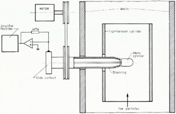
Fig.1. Experimental set-up.
Table I Experimental Conditions and Collision Parameters

3 Model For the Charge Separation
The experiments showed that the measured current depended on the kind of metal, and that there is a non-linear dependence on the electric field. To explain the first fact, there are different possibilities to consider, such as electrode processes in electrolytes, solvated electrons, or electronic surface states on the ice. In all three cases we must introduce electronic states whether they exist already in the ice or are only created in contact with the metal (Pikayev, 1969, p. 320-68 of the English translation). As the first two possibilities did not adequately describe the observations, they were ruled out. For comparison with other fields in solid-state physics, we have an abundant literature on semiconductor surfaces (Davison and Levine, 1970; Many and others, 1971). So the model is based on the following assumptions:
-
(a) There are electronic surface states on the ice that exist already on the free ice surface or arc at least created by the metal.
-
(b) There is a reaction between the electrons and the ice charge carriers at least during the contact. This gives us the possibility of describing the influence of the electric field by the concentration of the ice charge carriers and their transition probability.
-
(c) The influence of the charge in the surface states on the charge transfer is assumed to be time independent. This is done because the collision lime could not be varied, being nearly independent of the metal and the impact velocity.
3.1. Ice in an external electric field
The charge carriers in ice are ions and Bjerrum defects (Jaccard, 1959; Gränicher, 1963, Fletcher, 1970). Both are in such a low concentration that Boltzmann statistics apply. In an electric field, a space charge will build up, much the same as in a semiconductor. So we may use the formulae for the charge-carrier concentrations and the electric potential derived there (e.g. Many and others, 1971, p. 138 ff.). We will consider the one-dimensional case only. The equations are written dimensionless with the units given in Table II.
Table II Units used for Dimensionless Quantities

For the concentration of the charge carriers we find
for the potential at the surface of the ice (Many and others, 1971)
where FE is the external electric field, and $$ is the permittivity.
3.2. Contact metal-ice
In describing the behaviour of the electrons in metals and semiconductors, the notion of the Fermi energy plays a dominant role. So we consider first the simple case of a contact where no charge separation is observed. This gives us the possibility of calculating the charge transferred by other metals. Next we calculate the influence of the electric field, starting again with a metal yielding no charge separation without an electric field. For the general case we combine the two parts.
3.2.1. Influence of the metal
In the case in which we find a metal without charge separation when in contact with ice, the charge carriers of this metal are in chemical equilibrium with those of the ice, even before contact occurred. This we use for the definition of the chemical potential ζ for the charge carriers of the ice, since in this case it is equal to the Fermi potential of the electrons in the metal. If we introduce the notion of the work function and fix the zero potential (vacuum level) in the usual way, we may say that the work function of the metal is equal to that in the ice. Thus we define the work function for ice and have at the same time a method of determining it. This method has been used to measure the work function of insulators (Davies, 1969).

Fig. 2. Definition of potential in metal and ice.
If we take another metal ($$ Fig. 2), we observe a charge transfer between the two contacting particles, which is explained by the principle of electrochemical equilibrium. This means that the difference in work function must equal the difference in the electrical potential. The charge connected with this potential is easily calculated if the charge distribution is known. To simplify the calculation, we assume that the whole charge lies in planes separated by some distance d, an assumption frequently also used in other fields (e.g. Hladik, 1972, p. 1092). As long as the whole charge is involved, the assumption pushes the problem of the charge distribution back to the distance d, since for any distribution d can be calculated. For the charge Q1 transferred per unit area we get
where $$
3.2.2. Influence of the external field ($$)
In this case we have already seen that there is no charge separation without an electric field: in equilibrium as many charges are being transferred from the metal to the ice as are transferred in the opposite direction. In other words the concentrations of the charge carriers are the same on both sides of the contact (n± = 1)· The electric field now changes the concentration in the ice, whereas in the metal, because of the high number of electrons, we still can assume n = 1. This leads to a charge transfer which we may imagine to be a chemical reaction involving L and D Bjerrum defects:
The charge separated is the net current flowing during the contact time. We calculate this current in the usual way by attributing transition probabilities to the charge carriers involved, evaluate the current for each in either direction, and add the currents up. We already know the concentrations from Equation (1) and we only have to introduce the transfer probabilities P+ and P– using the principle of microscopic reversibility for the direction and hoping to explain the experiments by a single kind of charge carriers in the ice (either ions or Bjerrum defects). Instead of P± we change to two other parameters (P0 and $$), defined by the equation
where η accounts for the difference in the transition probability for positive and negative charge carriers. Thus η may depend on the metal through the charge built up in the surface states of the ice.
The whole (negative) charge Q2 transferred over the distance d is calculated in the usual way, being the sum of all the concentrations multiplied by the corresponding transfer probability. Using the addition theorems for hyperbolic functions, we find at last (Buser, unpublished)
3.2.3. General case
In general we have $$. There is a charge transfer in the surface states Q1 and one induced by the electric field Q2. The whole charge is the sum of both of these, calculated using the equations above under the assumption that the transfer from the space-charge region of the ice is much slower than the transfer from the surface states. The total charge transferred Qt in dimensionless form can be written as
4. Results
Dimensions have to be given to the formulae derived if we want to compare with experiments. We will find that of all the parameters introduced, only four remain independent. These will be fitted with the experimental data by the $$-method. Since the four parameters are composed of geometrical (collision) and ice (concentration) parameters, we check the plausibility of the model. Another check will be the dependence of the parameters on the different metals.
4.1. Adjustment of the dimensionless equations
The dimensionless charge Q2 of Equation (5) gives the charge density in A s/m2 if we multiply by (q0/L2). With the contact area Ap for each particle and nt particles colliding per second, we find for the experimental current JE
Since FE is proportional to the applied voltage VE, we write Equation (2) with D as a constant and for X = D VE
Using the addition theorem for hyperbolic functions we get for the experimental current (Buser, unpublished)
with the four parameters to be fitted

JE0 is obviously just the field-independent part of the current, corresponding to the charges Q1 exchanged between the surface states of the ice and the metal. The quantity s is a number ≤1 allowing for charges which may How back from the surface states during the recoil of the ice particle (opening of the contact).
4.2. Discussion of the parameters
If we look closer at the four parameters, we see that D does not depend on the metal. Of course it depends on the geometrical arrangement, but as this is not changed in our experiments, D should remain constant.
Similarly JE0 should only depend on the metal, since nt remains constant, A ρ does not depend on the metal as long as it is harder than ice, which is true for most metals (exceptions: Pb, In). The distance d however may depend on the metal because there might be a different thickness of oxide or adsorption layers for different metals, thus showing the dependence on the metal is not only given by their work-function difference w.
The parameter A should not depend on the metal, except through a possible variation in the distance d as explained above. A depends on the concentration of the ice charge carriers, allowing us to decide whether Bjerrum- or ionic-defects are involved.
4.3. Measurements
The values of the parameters for 14 different cases are given in Table III. The metals are indicated by their chemical symbols. The letters in parentheses mean: (A) aged surface, Pd(H) is Pd filled with hydrogen. As discussed in the previous section, Table III shows that A and D do not depend much on the metal, but JE0 and η do.

Fig. 3. JE plotted against Vs/or Mg.
Table III Values of the Parameters

Figure 3 is an example of the measured current as a function of the applied voltage together with the fitted function from Equation (9). To show the fit for different metals, Equation (9) is transformed to the linear equation Z = $$ with
For better readability the result is shown in two parts (Figs 4 and 5) containing for the same reason three experimental points for each metal only (including extreme ones).

Fig. 4. Linear representation of Equation (9) for different metals (part 1).

Fig. 5. Linear representation of Equation (9) for different metals (part 2).

Fig. 6. Relation between η and JE0.
Since η may depend on the charge in the surface states (given by JE0) Figure 6 is given to show this relation, indicating that the transfer probabilities are influenced by a changing potential barrier.
5. Plausibility of the Model
In the previous section we saw that Equation (7) describes the experiments well if the proper values of the parameters are chosen. The question remains whether these values are consistent with the quantities they are composed of.
First we calculate the density of surface states. Since there are to our knowledge no data available for ice yet, we will compare it with known values for semiconductors and insulators. From the relation for the surface charge density σ
where N 1 is the density of surface states, we can evaluate N 1. As no saturation is observed in the experiments, we can only give a lower limit for N 1, using the maximum value of JE0(=3 nA). The quantity A p is known from collision theory, and nt from the experiment. With A = 16 x 10–12m2 and nt =105 s–1 we find 1016 m–2.
Many and others (1971, p. 358, 361) report 1017 m-2 for semiconductors while for insulators we find values of about 1014m-2 (Donald, 1968; Cunningham and Hood, 1970; Hood and Cunningham, 1970). Thus the value found seems to be reasonable.
Next we are able to decide on the kind of the ice charge carriers. For the moving ice particles, the inhomogeneous field is variable. Due to the different relaxation time of ionic and Bjerrum defects, the calculation shows that the contribution of the Bjerrum defects exceeds the ionic one. But this argument is not decisive, so let us calculate the concentration with the help of Equations (2) and (8). Allowing for dimensions, we find
Taking the experimental values for X = 1, e.g. VE = 10 kV, D = 1 kV–1 and FE = 2.5 x 10⁶ V/m, the Debye length and the concentration are
the majority carrier giving $$ = 3,
This value is to be compared with the defect concentrations in pure ice at — 45°C:
If we allow for the impurity of the water used in the present case, we arrive at the conclusion that the Bjerrum defects react with the metal electrons (Von Hippel, 1971).
Finally we will give an estimate of the work function $$ for ice. For the work function of the metal $$ we are restricted to values reported in the literature. The scatter, especially of earlier values, may be due to uncontrolled surface conditions, which are not known in our case either. So the estimate for $$ is about 4.4 eV, a value which is close to that reported earlier (Buser and Aufdermaur, 1971 ) and confirmed recently (Mazzega and others, 1976).
6. Conclusion
The proposed model explaining the charge transfer between metals and ice leads to two conclusions:
-
There are electron states on the surface of the ice.
-
Bjerrum defects react with the electrons exchanged with the metal.
Even though the experiments were not intended to investigate electrode processes at a metal ice interface, they proved to be quite a good start, since the contact time is short enough to see the initial stage of the charge transfer. It was just this short time of contact that allowed us to distinguish between the charging of surface states and the charge exchange between the space-charge layer in the ice and electrons in the metal. But the above conclusions have still to be confirmed by other experiments.
7. Acknowledgements
The experiments were performed at the Eidg. Institut für Scbnee- und Lawinenforschung; support by the Schweizerischer Nationalfonds zur Förderung der wissenschaftlicbe Forschung (Project No. 2.377.70) and the Schweizerische Hagelversicherungsgesellschaft, is gratefully acknowledged.
Discussion
G. W. GROSS: Von Hippel and others (1972) have suggested that electrons incident at the surface of an ice particle with sufficient energy may convert Bjerrum defects into ions (and vice versa). Latham and Mason (1961) performed experiments on the electric charge separation in ice/ice particle collisions in the absence of liquid water and found that an electric field has no effect. They ascribed that to a particle contact time smaller than the relaxation time for charge transfer

where $$e0 is the permittivity of free space, $$tr the principal relative dielectric constant of ice, and σ0 the static conductivity of ice. Based on my own measurements of their relaxation time, I suspect that this reason is incorrect. What mechanism would you propose for charge transfer in ice/ice collisions, other than a thermoelectric effect?
O. BUSER: Since I suggest electronic surface states on the ice, two ice particles are able to transfer electrons between their surface states. A net charge transfer may be observed whenever there exists a difference in their work function. This difference is very much dependent on the surface condition; changing by about 200-300 meV for an evaporated and a deposited ice surface. In this case the influence of the electric field is indeed small, which is readily verified by Equation (9) with η≈ 0.
F. PRODI: AS further comment on the applicability of the experiment to thunderstorm electricity, I recall that charge exchange between colliding ice particles is not a very effective mechanism in thunderstorms, as a recent experiment by Takahashi demonstrates.
BUSER: My paper is not intended to be a contribution to thunderstorm electricity, but to give insight into the fundamental physical processes involved in metal-ice interfaces.


